
CHAPTER 19
Numerics in General

Numeric analysis or briefly numerics has a distinct flavor that is different from basic calculus, from solving ODEs algebraically, or from other (nonnumeric) areas. Whereas in calculus and in ODEs there were very few choices on how to solve the problem and your answer was an algebraic answer, in numerics you have many more choices and your answers are given as tables of values (numbers) or graphs. You have to make judicous choices as to what numeric method or algorithm you want to use, how accurate you need your result to be, with what value (starting value) do you want to begin your computation, and others. This chapter is designed to provide a good transition from the algebraic type of mathematics to the numeric type of mathematics.
We begin with the general concepts such as floating point, roundoff errors, and general numeric errors and their propagation. This is followed in Sec. 19.2 by the important topic of solving equations of the type f(x) = 0 by various numeric methods, including the famous Newton method. Section 19.3 introduces interpolation methods. These are methods that construct new (unknown) function values from known function values. The knowledge gained in Sec. 19.3 is applied to spline interpolation (Sec. 19.4) and is useful for understanding numeric integration and differentiation covered in the last section.
Numerics provides an invaluable extension to the knowledge base of the problem-solving engineer. Many problems have no solution formula (think of a complicated integral or a polynomial of high degree or the interpolation of values obtained by measurements). In other cases a complicated solution formula may exist but may be practically useless. It is for these kinds of problems that a numerical method may generate a good answer. Thus, it is very important that the applied mathematician, engineer, physicist, or scientist becomes familiar with the essentials of numerics and its ideas, such as estimation of errors, order of convergence, numerical methods expressed in algorithms, and is also informed about the important numeric methods.
Prerequisite: Elementary calculus.
References and Answers to Problems: App. 1 Part E, App. 2.
19.1 Introduction
As an engineer or physicist you may deal with problems in elasticity and need to solve an equation such as x cosh x = 1 or a more difficult problem of finding the roots of a higher order polynomial. Or you encounter an integral such as

[see App. 3, formula (35)] that you cannot solve by elementary calculus. Such problems, which are difficult or impossible to solve algebraically, arise frequently in applications. They call for numeric methods, that is, systematic methods that are suitable for solving, numerically, the problems on computers or calculators. Such solutions result in tables of numbers, graphical representation (figures), or both. Typical numeric methods are iterative in nature and, for a well-choosen problem and a good starting value, will frequently converge to a desired answer. The evolution from a given problem that you observed in an experimental lab or in an industrial setting (in engineering, physics, biology, chemistry, economics, etc.) to an approximation suitable for numerics to a final answer usually requires the following steps.
- Modeling. We set up a mathematical model of our problem, such as an integral, a system of equations, or a differential equation.
- Choosing a numeric method and parameters (e.g., step size), perhaps with a preliminary error estimation.
- Programming. We use the algorithm to write a corresponding program in a CAS, such as Maple, Mathematica, Matlab, or Mathcad, or, say, in Java, C or C++, or FORTRAN, selecting suitable routines from a software system as needed.
- Doing the computation.
- Interpreting the results in physical or other terms, also deciding to rerun if further results are needed.
Steps 1 and 2 are related. A slight change of the model may often admit of a more efficient method. To choose methods, we must first get to know them. Chapters 19–21 contain efficient algorithms for the most important classes of problems occurring frequently in practice.
In Step 3 the program consists of the given data and a sequence of instructions to be executed by the computer in a certain order for producing the answer in numeric or graphic form.
To create a good understanding of the nature of numeric work, we continue in this section with some simple general remarks.
Floating-Point Form of Numbers
We know that in decimal notation, every real number is represented by a finite or an infinite sequence of decimal digits. Now most computers have two ways of representing numbers, called fixed point and floating point. In a fixed-point system all numbers are given with a fixed number of decimals after the decimal point; for example, numbers given with 3 decimals are 62.358, 0.014, 1.000. In a text we would write, say, 3 decimals as 3D. Fixed-point representations are impractical in most scientific computations because of their limited range (explain!) and will not concern us.
In a floating-point system we write, for instance,
![]()
or sometimes also
![]()
We see that in this system the number of significant digits is kept fixed, whereas the decimal point is “floating.” Here, a significant digit of a number c is any given digit of c, except possibly for zeros to the left of the first nonzero digit; these zeros serve only to fix the position of the decimal point. (Thus any other zero is a significant digit of c.) For instance,
![]()
all have 5 significant digits. In a text we indicate, say, 5 significant digits, by 5S.
The use of exponents permits us to represent very large and very small numbers. Indeed, theoretically any nonzero number a can be written as
![]()
On modern computers, which use binary (base 2) numbers, m is limited to k binary digits (e.g., k = 8) and n is limited (see below), giving representations (for finitely many numbers only!)
![]()
These numbers ![]() are called k-digit binary machine numbers. Their fractional part m (or
are called k-digit binary machine numbers. Their fractional part m (or ![]() ) is called the mantissa. This is not identical with “mantissa” as used for logarithms. n is called the exponent of
) is called the mantissa. This is not identical with “mantissa” as used for logarithms. n is called the exponent of ![]() .
.
It is important to realize that there are only finitely many machine numbers and that they become less and less “dense” with increasing a. For instance, there are as many numbers between 2 and 4 as there are between 1024 and 2048. Why?
The smallest positive machine number eps with 1 + eps > 1 is called the machine accuracy. It is important to realize that there are no numbers in the intervals [1, 1 + eps], [2, 2 + 2 · eps], …, [1024, 1024 + 1024 · eps], …. This means that, if the mathematical answer to a computation would be 1024 + 1024 · eps/2, the computer result will be either 1024 or 1024 · eps so it is impossible to achieve greater accuracy.
Underflow and Overflow. The range of exponents that a typical computer can handle is very large. The IEEE (Institute of Electrical and Electronic Engineers) floating-point standard for single precision is from 2−126 to 2128 (1.175 × 10−38 to 3.403 × 1038) and for double precision it is from 2−1022 to 21024 (2.225 × 10−308 to 1.798 × 10308).
As a minor technicality, to avoid storing a minus in the exponent, the ranges are shifted from [− 126. 128] by adding 126 (for double precision 1022). Note that shifted exponents of 255 and 1047 are used for some special cases such as representing infinity.
If, in a computation a number outside that range occurs, this is called underflow when the number is smaller and overflow when it is larger. In the case of underflow, the result is usually set to zero and computation continues. Overflow might cause the computer to halt. Standard codes (by IMSL, NAG, etc.) are written to avoid overflow. Error messages on overflow may then indicate programming errors (incorrect input data, etc.). From here on, we will be discussing the decimal results that we obtain from our computations.
Roundoff
An error is caused by chopping (= discarding all digits from some decimal on) or rounding. This error is called roundoff error, regardless of whether we chop or round. The rule for rounding off a number to k decimals is as follows. (The rule for rounding off to k significant digits is the same, with “decimal” replaced by “significant digit.”)
Roundoff Rule. To round a number x to k decimals, and 5 · 10−(k+1) to x and chop the digits after the (k + 1)st digit.
Round the number 1.23454621 to (a) 2 decimals, (b) 3 decimals, (c) 4 decimals, (d) 5 decimals, and (e) 6 decimals.
Solution. (a) For 2 decimals we add 5 · 10−(k+1) = 5 · 10−3 = 0.005 to the given number, that is, 1.2345621 + 0.005 = 1.23 954621. Then we chop off the digits “954621” after the space or equivalently 1.23954621 − 0.00954621 = 1.23.
- (b) 1.23454621 + 0.0005 = 1.235 04621, so that for 3 decimals we get 1.234.
- (c) 1.23459621 after chopping give us 1.2345 (4 decimals).
- (d) 1.23455121 yields 1.23455 (5 decimals).
- (e) 1.23454671 yields 1.234546 (6 decimals).
Can you round the number to 7 decimals?
Chopping is not recommended because the corresponding error can be larger than that in rounding. (Nevertheless, some computers use it because it is simpler and faster. On the other hand, some computers and calculators improve accuracy of results by doing intermediate calculations using one or more extra digits, called guarding digits.)
Error in Rounding. Let ![]() = fl (a) in (2) be the floating-point computer approximation of a in (1) obtained by rounding, where fl suggests floating. Then the roundoff rule gives (by dropping exponents)
= fl (a) in (2) be the floating-point computer approximation of a in (1) obtained by rounding, where fl suggests floating. Then the roundoff rule gives (by dropping exponents) ![]() Since |m|
Since |m| ![]() 0.1, this implies (when a ≠ 0)
0.1, this implies (when a ≠ 0)

The right side ![]() is called the rounding unit. If we write
is called the rounding unit. If we write ![]() = a(1 + δ), we have by algebra (
= a(1 + δ), we have by algebra (![]() − a)/a = δ, hence |δ|
− a)/a = δ, hence |δ| ![]() u by (3). This shows that the rounding unit u is an error bound in rounding.
u by (3). This shows that the rounding unit u is an error bound in rounding.
Rounding errors may ruin a computation completely, even a small computation. In general, these errors become the more dangerous the more arithmetic operations (perhaps several millions!) we have to perform. It is therefore important to analyze computational programs for expected rounding errors and to find an arrangement of the computations such that the effect of rounding errors is as small as possible.
As mentioned, the arithmetic in a computer is not exact and causes further errors; however, these will not be relevant to our discussion.
Accuracy in Tables. Although available software has rendered various tables of function values superfluous, some tables (of higher functions, of coefficients of integration formulas, etc.) will still remain in occasional use. If a table shows k significant digits, it is conventionally assumed that any value ![]() in the table deviates from the exact value a by at most
in the table deviates from the exact value a by at most ![]() unit of the kth digit.
unit of the kth digit.
Loss of Significant Digits
This means that a result of a calculation has fewer correct digits than the numbers from which it was obtained. This happens if we subtract two numbers of about the same size, for example, 0.1439 − 0.1426 (“subtractive cancellation”). It may occur in simple problems, but it can be avoided in most cases by simple changes of the algorithm—if one is aware of it! Let us illustrate this with the following basic problem.
EXAMPLE 2 Quadratic Equation. Loss of Significant Digits
Find the roots of the equation
![]()
using 4 significant digits (abbreviated 4S) in the computation.
Solution. A formula for the roots x1, x2 of a quadratic equation ax2 + bx + c = 0 is
![]()
Furthermore, since x1x2 = c/a, another formula for those roots
![]()
We see that this avoids cancellation in x1 for positive b.
If b < 0, calculate x1 from (4) and then x2 = c/(ax1).
For x2 + 40x + 2 = 0 we obtain from (4) ![]() hence x2 = −20.00 − 19.95, involving no difficulty, and x1 = −20.00 + 19.95 = −0.05, a poor value involving loss of digits by subtractive cancellation.
hence x2 = −20.00 − 19.95, involving no difficulty, and x1 = −20.00 + 19.95 = −0.05, a poor value involving loss of digits by subtractive cancellation.
In contrast, (5) gives x1 = 2.000/(−39.95) = −0.05006, the absolute value of the error being less than one unit of the last digit, as a computation with more digits shows. The 10S-value is −0.05006265674.
Errors of Numeric Results
Final results of computations of unknown quantities generally are approximations; that is, they are not exact but involve errors. Such an error may result from a combination of the following effects. Roundoff errors result from rounding, as discussed above. Experimental errors are errors of given data (probably arising from measurements). Truncating errors result from truncating (prematurely breaking off), for instance, if we replace a Taylor series with the sum of its first few terms. These errors depend on the computational method used and must be dealt with individually for each method. [“Truncating” is sometimes used as a term for chopping off (see before), a terminology that is not recommended.]
Formulas for Errors. If ![]() is an approximate value of a quantity whose exact value is a, we call the difference
is an approximate value of a quantity whose exact value is a, we call the difference

the error of ![]() . Hence
. Hence

For instance, if ![]() = 10.5 is an approximation of a = 10.2, its error is
= 10.5 is an approximation of a = 10.2, its error is ![]() = −0.3. The error of an approximation
= −0.3. The error of an approximation ![]() = 1.60 of a = 1.82 is
= 1.60 of a = 1.82 is ![]() = 0.22.
= 0.22.
CAUTION! In the literature ![]() (“absolute error”) or
(“absolute error”) or ![]() are sometimes also used as definitions of error.
are sometimes also used as definitions of error.
The relative error ![]() r of
r of ![]() is defined by
is defined by

This looks useless because a is unknown. But if |![]() | is much less than |
| is much less than |![]() |, then we can use
|, then we can use ![]() instead of a and get
instead of a and get
![]()
This still looks problematic because ![]() is unknown—if it were known, we could get
is unknown—if it were known, we could get ![]() from (6) and we would be done. But what one often can obtain in practice is an error bound for
from (6) and we would be done. But what one often can obtain in practice is an error bound for ![]() , that is, a number β such that
, that is, a number β such that
![]()
This tells us how far away from our computed ![]() the unknown a can at most lie. Similarly, for the relative error, an error bound is a number βr such that
the unknown a can at most lie. Similarly, for the relative error, an error bound is a number βr such that

Error Propagation
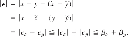
This is an important matter. It refers to how errors at the beginning and in later steps (roundoff, for example) propagate into the computation and affect accuracy, sometimes very drastically. We state here what happens to error bounds. Namely, bounds for the error add under addition and subtraction, whereas bounds for the relative error add under multiplication and division. You do well to keep this in mind.
(a) In addition and subtraction, a bound for the error of the results is given by the sum of the error bounds for the terms.
(b) In multiplication and division, an error bound for the relative error of the results is given (approximately) by the sum of the bounds for the relative errors of the given numbers.
PROOF
(a) We use the notations ![]() Then for the error
Then for the error ![]() of the difference we obtain
of the difference we obtain
The proof for the sum is similar and is left to the student.
(b) For the relative error ![]() r of
r of ![]() we get from the relative errors
we get from the relative errors ![]() rx and
rx and ![]() ry of
ry of ![]() and bounds βrx, βry
and bounds βrx, βry

This proof shows what “approximately” means: we neglected ![]() x
x![]() y as small in absolute value compared to |
y as small in absolute value compared to |![]() x| and |
x| and |![]() y|. The proof for the quotient is similar but slightly more tricky (see Prob. 13).
y|. The proof for the quotient is similar but slightly more tricky (see Prob. 13).
Basic Error Principle
Every numeric method should be accompanied by an error estimate. If such a formula is lacking, is extremely complicated, or is impractical because it involves information (for instance, on derivatives) that is not available, the following may help.
Error Estimation by Comparison. Do a calculation twice with different accuracy. Regard the difference ![]() of the results
of the results ![]() as a (perhaps crude) estimate of the error
as a (perhaps crude) estimate of the error ![]() 1 of the inferior result
1 of the inferior result ![]() Indeed,
Indeed, ![]() by formula (4*). This implies
by formula (4*). This implies ![]() because
because ![]() is generally more accurate than
is generally more accurate than ![]() so that |
so that |![]() 2| is small compared to |
2| is small compared to |![]() 1|.
1|.
Algorithm. Stability
Numeric methods can be formulated as algorithms. An algorithm is a step-by-step procedure that states a numeric method in a form (a “pseudocode”) understandable to humans. (See Table 19.1 to see what an algorithm looks like.) The algorithm is then used to write a program in a programming language that the computer can understand so that it can execute the numeric method. Important algorithms follow in the next sections. For routine tasks your CAS or some other software system may contain programs that you can use or include as parts of larger programs of your own.
Stability. To be useful, an algorithm should be stable; that is, small changes in the initial data should cause only small changes in the final results. However, if small changes in the initial data can produce large changes in the final results, we call the algorithm unstable.
This “numeric instability,” which in most cases can be avoided by choosing a better algorithm, must be distinguished from “mathematical instability” of a problem, which is called “ill-conditioning,” a concept we discuss in the next section.
Some algorithms are stable only for certain initial data, so that one must be careful in such a case.
- Floating point. Write 84.175, −528.685, 0.000924138, and −362005 in floating-point form, rounded to 5S (5 significant digits).
- Write −76.437125, 60100, and −0.00001 in floating-point form, rounded to 4S.
- Small differences of large numbers may be particularly strongly affected by rounding errors. Illustrate this by computing 0.81534/(35 · 724 − 35.596) as given with 5S, then rounding stepwise to 4S, 3S, and 2S, where “stepwise” means round the rounded numbers, not the given ones.
- Order of terms, in adding with a fixed number of digits, will generally affect the sum. Give an example. Find empirically a rule for the best order.
- Rounding and adding. Let a1, …, an be numbers with aj correctly rounded to Sj digits. In calculating the sum a1 + … + an, retaining S = min Sj significant digits, is it essential that we first add and then round the result or that we first round each number to S significant digits and then add?
- Nested form. Evaluate
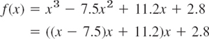
at x = 3.94 using 3S arithmetic and rounding, in both of the given forms. The latter, called the nested form, is usually preferable since it minimizes the number of operations and thus the effect of rounding.
- Quadratic equation. Solve x2 − 30x + 1 = 0 by (4) and by (5), using 6S in the computation. Compare and comment.
- Solve x2 − 40x + 2 = 0, using 4S-computation.
- Do the computations in Prob. 7 with 4S and 2S.
- Instability. For small |a| the equation (x − k)2 = a has nearly a double root. Why do these roots show instability?
- Theorems on errors. Prove Theorem 1(a) for addition.
- Overflow and underflow can sometimes be avoided by simple changes in a formula. Explain this in terms of
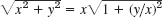 with x2
  y2 and x so large that x2 would cause overflow. Invent examples of your own.
 - Division. Prove Theorem 1(b) for division.
- Loss of digits. Square root. Compute
 with 6S arithmetic for x = 0.001 (a) as given and (b) from
  (derive!).
 - Logarithm. Compute ln a − ln b with 6S arithmetic for a = 4.00000 and b = 3.99900 (a) as given and (b) from ln(a/b).
- Cosine. Compute 1 − cos x with 6S arithmetic for x = 0.02 (a) as given and (b) by 2
 (derive!).
 - Discuss the numeric use of (12) in App. A3.1 for when cos v − cos u when u ≈ v.
- Quotient near 0/0. (a) Compute (1 − cos x)/sin x with 6S arithmetic for x = 0.005. (b) Looking at Prob. 16, find a much better formula.
- Exponential function. Calculate 1/e = 0.367879(6S) from the partial sums of 5–10 terms of the Maclaurin series (a) of e−x with x = 1, (b) of ex with x = 1 and then taking the reciprocal. Which is more accurate?
- Compute e−10 with 6S arithmetic in two ways (as in Prob. 19).
- Binary conversion. Show that

can be obtained by the division algorithm

- Convert (0.59375)10 to (0.10011)2 by successive multiplication by 2 and dropping (removing) the integer parts, which give the binary digits c1, c2, …:

- Show that 0.1 is not a binary machine number.
- Prove that any binary machine number has a finite decimal representation. Is the converse true?
- CAS EXPERIMENT. Approximations. Obtain
 from Prob. 23. Which machine number (partial sum) Sn will first have the value 0.1 to 30 decimal digits?
 - CAS EXPERIMENT. Integration from Calculus. Integrating by parts, show that
 e − nIn − 1, I0 = e − 1. (a) Compute In, n = 0, …, using 4S arithmetic, obtaining I8 = −3.906. Why is this nonsense? Why is the error so large?
(b) Experiment in (a) with the number of digits k > 4. As you increase k, will the first negative value n = N occur earlier or later? Find an empirical formula for N = N(k).
- Backward Recursion. In Prob. 26. Using ex < e (0 < x < 1), conclude that |In|
 e/(n + 1)→ 0 as n → ∞. Solve the iteration formula for In−1 = (e − In)/n, start from I15 ≈ 0 and compute 4S values of I14, I13, …, I1.
 - Harmonic series.
 diverges. Is the same true for the corresponding series of computer numbers?
 - Approximations of π = 3.14159265358979 … are 22/7 and 355/113. Determine the corresponding errors and relative errors to 3 significant digits.
- Compute π by Machin's approximation 16 arctab
 arctan
  to 10S (which are correct). [In 1986, D. H. Bailey (NASA Ames Research Center, Moffett Field, CA 94035) computed almost 30 million decimals of π on a CRAY-2 in less than 30 hrs. The race for more and more decimals is continuing. See the Internet under pi.]
19.2 Solution of Equations by Iteration
For each of the remaining sections of this chapter, we select basic kinds of problems and discuss numeric methods on how to solve them. The reader will learn about a variety of important problems and become familiar with ways of thinking in numerical analysis.
Perhaps the easiest conceptual problem is to find solutions of a single equation

where f is a given function. A solution of (1) is a number x = s such that f(s) = 0. Here, s suggests “solution,” but we shall also use other letters.
It is interesting to note that the task of solving (1) is a question made for numeric algorithms, as in general there are no direct formulas, except in a few simple cases.
Examples of single equations are x3 + x = 1, sin x = 0.5x, tan x = x, cosh x = sec x, cosh x cos x = −1, which can all be written in the form of (1). The first of the five equations is an algebraic equation because the corresponding f is a polynomial. In this case the solutions are called roots of the equation and the solution process is called finding roots. The other equations are transcendental equations because they involve transcendental functions.
There are a very large number of applications in engineering, where we have to solve a single equation (1). You have seen such applications when solving characteristic equations in Chaps. 2, 4, and 8; partial fractions in Chap. 6; residue integration in Chap. 16, finding eigenvalues in Chap. 12, and finding zeros of Bessel functions, also in Chap. 12. Moreover, methods of finding roots are very important in areas outside of classical engineering. For example, in finance, the problem of determining how much a bond is worth amounts to solving an algebraic equation.
To solve (1) when there is no formula for the exact solution available, we can use an approximation method, such as an iteration method. This is a method in which we start from an initial guess x0 (which may be poor) and compute step by step (in general better and better) approximations x1, x2, … of an unknown solution of (1). We discuss three such methods that are of particular practical importance and mention two others in the problem set.
It is very important that the reader understand these methods and their underlying ideas. The reader will then be able to select judiciously the appropriate software from among different software packages that employ variations of such methods and not just treat the software programs as “black boxes.”
In general, iteration methods are easy to program because the computational operations are the same in each step—just the data change from step to step—and, more importantly, if in a concrete case a method converges, it is stable in general (see Sec. 19.1).
Fixed-Point Iteration for Solving Equations f(x) = 0
Note: Our present use of the word “fixed point” has absolutely nothing to do with that in the last section.
By some algebraic steps we transform (1) into the form
![]()
Then we choose an x0 and compute x1 = g(x0), x2 = g(x1), and in general

A solution of (2) is called a fixed point of g, motivating the name of the method. This is a solution of (1), since from x = g(x) we can return to the original form f(x) = 0. From (1) we may get several different forms of (2). The behavior of corresponding iterative sequences x0, x1, … may differ, in particular, with respect to their speed of convergence. Indeed, some of them may not converge at all. Let us illustrate these facts with a simple example.
EXAMPLE 1 An Iteration Process (Fixed-Point Iteration)
Set up an iteration process for the equation f(x) = x2 − 3x + 1 = 0. Since we know the solutions
![]()
we can watch the behavior of the error as the iteration proceeds.
Solution. The equation may be written
![]()
If we choose x0 = 1, we obtain the sequence (Fig. 426a; computed with 6S and then rounded)
![]()
which seems to approach the smaller solution. If we choose x0 = 2, the situation is similar. If we choose x0 = 3, we obtain the sequence (Fig. 426a, upper part)
![]()
which diverges.
Our equation may also be written (divide by x)
![]()
and if we choose x0 = 1, we obtain the sequence (Fig. 426b)
![]()
which seems to approach the larger solution. Similarly, if we choose x0 = 3, we obtain the sequence (Fig. 426b)
![]()

Fig. 426. Example 1, iterations (4a) and (4b)
Our figures show the following. In the lower part of Fig. 426a the slope of g1(x) is less than the slope of y = x, which is 1, thus ![]() and we seem to have convergence. In the upper part, g1(x) is steeper
and we seem to have convergence. In the upper part, g1(x) is steeper ![]() and we have divergence. In Fig. 426b the slope of g2(x) is less near the intersection point (x = 2.618, fixed point of g2, solution of f(x) = 0), and both sequences seem to converge. From all this we conclude that convergence seems to depend on the fact that, in a neighborhood of a solution, the curve of g(x) is less steep than the straight line y = x, and we shall now see that this condition |g′(x)| < 1 (= slope of y = x) is sufficient for convergence.
and we have divergence. In Fig. 426b the slope of g2(x) is less near the intersection point (x = 2.618, fixed point of g2, solution of f(x) = 0), and both sequences seem to converge. From all this we conclude that convergence seems to depend on the fact that, in a neighborhood of a solution, the curve of g(x) is less steep than the straight line y = x, and we shall now see that this condition |g′(x)| < 1 (= slope of y = x) is sufficient for convergence.
An iteration process defined by (3) is called convergent for an x0 if the corresponding sequence x0, x1, … is convergent.
A sufficient condition for convergence is given in the following theorem, which has various practical applications.
THEOREM 1 Convergence of Fixed-Point Iteration
Let x = s be a solution of x = g(x) and suppose that g has a continuous derivative in some interval J containing s. Then, if |g′(x)| ![]() K < 1 in J, the iteration process defined by (3) converges for any x0 in J. The limit of the sequence {xn} is s.
K < 1 in J, the iteration process defined by (3) converges for any x0 in J. The limit of the sequence {xn} is s.
PROOF
By the mean value theorem of differential calculus there is a t between x and s such that
![]()
Since g(s) = s and x1 = g(x0), x2 = g(x1), …, we obtain from this and the condition on |g′(x)| in the theorem
![]()
Applying this inequality n times, for n, n − 1, …, 1 gives
![]()
Since K < 1, we have Kn → 0; hence |xn − s| → 0 as n → ∞.
We mention that a function g satisfying the condition in Theorem 1 is called a contraction because |g(x) − g(v)| ![]() K|x − v|, where K < 1. Furthermore, K gives information on the speed of convergence. For instance, if K = 0.5, then the accuracy increases by at least 2 digits in only 7 steps because 0.57 < 0.01.
K|x − v|, where K < 1. Furthermore, K gives information on the speed of convergence. For instance, if K = 0.5, then the accuracy increases by at least 2 digits in only 7 steps because 0.57 < 0.01.
EXAMPLE 2 An Iteration Process. Illustration of Theorem 1
Find a solution of f(x) = x3 + x − 1 = 0 by iteration.
Solution. A sketch shows that a solution lies near x = 1. (a) We may write the equation as (x2 + 1)x = 1 or

for any x because 4x2/(1 + x2)4 = 4x2/(1 + 4x2 + …) < 1, so that by Theorem 1 we have convergence for any x0. Choosing x0 = 1, we obtain (Fig. 427)
![]()
The solution exact to 6D is s = 0.682328.
(b) The given equation may also be written
![]()
and this is greater than 1 near the solution, so that we cannot apply Theorem 1 and assert convergence. Try x0 = 1, x0 = 0.5, x0 = 2 and see what happens.
The example shows that the transformation of a given f(x) = 0 into the form x = g(x) with g satisfying |g′(x) ![]() K < 1 may need some experimentation.
K < 1 may need some experimentation.
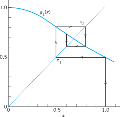
Fig. 427. Iteration in Example 2

Newton's Method for Solving Equations f(x) = 0
Newton's method, also known as Newton–Raphson's method,1 is another iteration method for solving equations f(x) = 0 where f is assumed to have a continuous derivative f′. The method is commonly used because of its simplicity and great speed.
The underlying idea is that we approximate the graph of f by suitable tangents. Using an approximate value x0 obtained from the graph of f, we let x1 be the point of intersection of the x-axis and the tangent to the curve of f at x0 (see Fig. 428). Then
![]()
In the second step we compute x2 = x1 − f(x1)/f′(x1), in the third step x3 from x2 again by the same formula, and so on. We thus have the algorithm shown in Table 19.1. Formula (5) in this algorithm can also be obtained if we algebraically solve Taylor's formula
![]()
Table 19.1 Newton's Method for Solving Equations f(x) = 0

If it happens that f′(xn) = 0 for some n (see line 2 of the algorithm), then try another starting value x0. Line 3 is the heart of Newton's method.
The inequality in line 4 is a termination criterion. If the sequence of the xn converges and the criterion holds, we have reached the desired accuracy and stop. Note that this is just a form of the relative error test. It ensures that the result has the desired number of significant digits. If |xn+1| = 0, the condition is satisfied if and only if xn+1 = xn = 0, otherwise |xn+1 − xn| must be sufficiently small. The factor |xn+1| is needed in the case of zeros of very small (or very large) absolute value because of the high density (or of the scarcity) of machine numbers for those x.
WARNING! The criterion by itself does not imply convergence. Example. The harmonic series diverges, although its partial sums ![]() satisfy the criterion because lim (xn+1 − xn) = lim (1/(n + 1)) = 0.
satisfy the criterion because lim (xn+1 − xn) = lim (1/(n + 1)) = 0.
Line 5 gives another termination criterion and is needed because Newton's method may diverge or, due to a poor choice of x0, may not reach the desired accuracy by a reasonable number of iterations. Then we may try another x0. If f(x) = 0 has more than one solution, different choices of x0 may produce different solutions. Also, an iterative sequence may sometimes converge to a solution different from the expected one.
Set up a Newton iteration for computing the square root x of a given positive number c and apply it to c = 2.
Solution. We have ![]() hence f(x) = x2 − c = 0,f′(x) = 2x, and (5) takes the form
hence f(x) = x2 − c = 0,f′(x) = 2x, and (5) takes the form
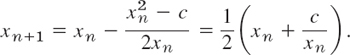
For c = 2, choosing x0 = 1, we obtain
![]()
x4 is exact to 6D.
EXAMPLE 4 Iteration for a Transcendental Equation
Find the positive solution of 2 sin x = x.
Solution. Setting f(x) = x − 2 sin x, we have f′(x) = 1 − 2 cos x, and (5) gives
![]()

From the graph of f we conclude that the solution is near x0 = 2. We compute: x4 = 1.89549 is exact to 5D since the solution to 6D is 1.895494.
EXAMPLE 5 Newton's Method Applied to an Algebraic Equation
Apply Newton's method to the equation f(x) = x2 + x − 1 = 0.
Solution. From (5) we have
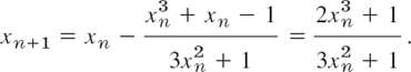
Starting from x0 = 1, we obtain
![]()
where x4 has the error −1 · 10−6. A comparison with Example 2 shows that the present convergence is much more rapid. This may motivate the concept of the order of an iteration process, to be discussed next.
Order of an Iteration Method. Speed of Convergence
The quality of an iteration method may be characterized by the speed of convergence, as follows.
Let xn+1 = g(xn) define an iteration method, and let xn approximate a solution s of x = g(x). Then xn = s − ![]() n, where
n, where ![]() n is the error of xn. Suppose that g is differentiable a number of times, so that the Taylor formula gives
n is the error of xn. Suppose that g is differentiable a number of times, so that the Taylor formula gives

The exponent of ![]() n in the first nonvanishing term after g(s) is called the order of the iteration process defined by g. The order measures the speed of convergence.
n in the first nonvanishing term after g(s) is called the order of the iteration process defined by g. The order measures the speed of convergence.
To see this, subtract g(s) = s on both sides of (6). Then on the left you get xn+1 − s = −![]() n+1, where
n+1, where ![]() n+1 is the error of xn+1. And on the right the remaining expression equals approximately its first nonzero term because |
n+1 is the error of xn+1. And on the right the remaining expression equals approximately its first nonzero term because |![]() n| is small in the case of convergence. Thus
n| is small in the case of convergence. Thus

Thus if ![]() n = 10−k in some step, then for second order,
n = 10−k in some step, then for second order, ![]() n+1 = c · (10−k)2 = c · 10−2k, so that the number of significant digits is about doubled in each step.
n+1 = c · (10−k)2 = c · 10−2k, so that the number of significant digits is about doubled in each step.
Convergence of Newton's Method
In Newton's method, g(x) = x − f(x)/f′(x). By differentiation,

Since f(s) = 0, this shows that also g′(s) = 0. Hence Newton's method is at least of second order. If we differentiate again and set x = s, we find that
which will not be zero in general. This proves
THEOREM 2 Second-Order Convergence of Newton's Method
If f(x) is three times differentiable and f′ and f″ are not zero at a solution s of f(x) = 0, then for x0 sufficiently close to s, Newton's method is of second order.
Comments. For Newton's method, (7b) becomes, by (8*)

For the rapid convergence of the method indicated in Theorem 2 it is important that s be a simple zero of f(x) (thus f′(s) ≠ 0) and that x0 be close to s, because in Taylor's formula we took only the linear term [see (5*)], assuming the quadratic term to be negligibly small. (With a bad x0 the method may even diverge!)
EXAMPLE 6 Prior Error Estimate of the Number of Newton Iteration Steps
Use x0 = 2 and x1 = 1.901 in Example 4 for estimating how many iteration steps we need to produce the solution to 5D-accuracy. This is an a priori estimate or prior estimate because we can compute it after only one iteration, prior to further iterations.
Solution. We have f(x) = x − 2 sin x = 0. Differentiation gives

Hence (9) gives
![]()
where M = 2n + 2n−1 + … + 2 + 1 = 2n+1 − 1. We show below that ![]() 0 ≈ −0.11. Consequently, our condition becomes
0 ≈ −0.11. Consequently, our condition becomes
![]()
Hence n = 2 is the smallest possible n, according to this crude estimate, in good agreement with Example 4. ![]() 0 ≈ −0.11 is obtained from
0 ≈ −0.11 is obtained from ![]() 1 −
1 − ![]() 0 = (
0 = (![]() 1 − s) − (
1 − s) − (![]() 0 − s) = −x1 + x0 ≈ 0.10, hence
0 − s) = −x1 + x0 ≈ 0.10, hence ![]()
![]() which gives
which gives ![]() 0 ≈ −0.11.
0 ≈ −0.11.
Difficulties in Newton's Method. Difficulties may arise if |f′(x)| is very small near a solution s of f(x) = 0. For instance, let s be a zero of f(x) of second or higher order. Then Newton's method converges only linearly, as is shown by an application of l'Hopital's rule to (8). Geometrically, small |f′(x)| means that the tangent of f(x) near s almost coincides with the x-axis (so that double precision may be needed to get f(x) and f′(x) accurately enough). Then for values ![]() far away from s we can still have small function values
far away from s we can still have small function values
![]()
In this case we call the equation f(x) = 0 ill-conditioned. ![]() is called the residual of f(x) = 0 at
is called the residual of f(x) = 0 at ![]() . Thus a small residual guarantees a small error of
. Thus a small residual guarantees a small error of ![]() only if the equation is not ill-conditioned.
only if the equation is not ill-conditioned.
EXAMPLE 7 An Ill-Conditioned Equation
f(x) = x5 + 10−4x = 0 is ill-conditioned, x = 0 is a solution. f′(0) = 10−4 is small. At ![]() = 0.1 the residual f(0.1) = 2 · 10−5 is small, but the error −0.1 is larger in absolute value by a factor 5000. Invent a more drastic example of your own.
= 0.1 the residual f(0.1) = 2 · 10−5 is small, but the error −0.1 is larger in absolute value by a factor 5000. Invent a more drastic example of your own.
Secant Method for Solving f(x) = 0
Newton's method is very powerful but has the disadvantage that the derivative f′ may sometimes be a far more difficult expression than f itself and its evaluation therefore computationally expensive. This situation suggests the idea of replacing the derivative with the difference quotient
![]()
Then instead of (5) we have the formula of the popular secant method


Geometrically, we intersect the x-axis at xn+1 with the secant of f(x) passing through Pn−1 and Pn in Fig. 429. We need two starting values x0 and x1. Evaluation of derivatives is now avoided. It can be shown that convergence is superlinear (that is, more rapid than linear, |![]() n+1| ≈ const · |
n+1| ≈ const · |![]() n|1.62; see [E5] in App. 1), almost quadratic like Newton's method. The algorithm is similar to that of Newton's method, as the student may show.
n|1.62; see [E5] in App. 1), almost quadratic like Newton's method. The algorithm is similar to that of Newton's method, as the student may show.
CAUTION! It is not good to write (10) as
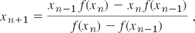
because this may lead to loss of significant digits if xn and xn−1 are about equal. (Can you see this from the formula?)
Find the positive solution of f(x) = x − 2 sin x = 0 by the secant method, starting from x0 = 2, x1 = 1.9
Solution. Here, (10) is

Numeric values are:

x3 = 1.895494 is exact to 6D. See Example 4.
Summary of Methods. The methods for computing solutions s of f(x) = 0 with given continuous (or differentiable) f(x) start with an initial approximation x0 of s and generate a sequence x1, x2, … by iteration. Fixed-point methods solve f(x) = 0 written as x = g(x), so that s is a fixed point of g, that is, s = g(s). For g(x) = x − f(x)/f′(x) this is Newton's method, which, for good x0 and simple zeros, converges quadratically (and for multiple zeros linearly). From Newton's method the secant method follows by replacing f′(x) by a difference quotient. The bisection method and the method of false position in Problem Set 19.2 always converge, but often slowly.
1–13 FIXED-POINT ITERATION
Solve by fixed-point iteration and answer related questions where indicated. Show details.
- Monotone sequence. Why is the sequence in Example 1 monotone? Why not in Example 2?
- Do the iterations (b) in Example 2. Sketch a figure similar to Fig. 427. Explain what happens.
- f = x − 0.5 cos x = 0, x0 = 1. Sketch a figure.
- f = x − cosec x the zero near x = 1
- Sketch f(x) = x3 − 5.00x2 + 1.01x + 1.88, showing roots near ±1 and 5. Write x = g(x) = (5.00x2 − 1.01x + 1.88)/x2. Find a root by starting from x0 = 5, 4, 1, −1. Explain the (perhaps unexpected) results.
- Find a form x = g(x) of f(x) = 0 in Prob. 5 that yields convergence to the root near x = 1.
- Find the smallest positive solution of sin x = e−x
- Solve x4 − x − 0.12 = 0 by starting from x0 = 1.
- Find the negative solution of x4 − x − 0.12 = 0.
- Elasticity. Solve x cosh x = 1. (Similar equations appear in vibrations of beams; see Problem Set 12.3.)
- Drumhead. Bessel functions. A partial sum of the Maclaurin series of J0(x) (Sec. 5.5) is

 Conclude from a sketch that f(x) = 0 near x = 2. Write f(x) = 0 as x = g(x) (by dividing f(x) by
  and taking the resulting x-term to the other side). Find the zero. (See Sec. 12.10 for the importance of these zeros.)
 - CAS EXPERIMENT. Convergence. Let f(x) = x3 + 2x2 − 3x − 4 = 0. Write this as x = g(x), for g choosing (1) (x3 − f)1/3, (2)
 (3)
(3)  (4) (x3 − f)/x2, (5) (2x2 − f)/(2x), and (6) x − f/f′ and in each case x0 = 1.5. Find out about convergence and divergence and the number of steps to reach 6S-values of a root.
 - Existence of fixed point. Prove that if g is continuous in a closed interval I and its range lies in I, then the equation x = g(x) has at least one solution in I. Illustrate that it may have more than one solution in I.
14–23 NEWTON'S METHOD
Apply Newton's method (6S-accuracy). First sketch the function(s) to see what is going on.
- 14. Cube root. Design a Newton iteration. Compute

- 15. f = 2x − cos x, x0 = 1. Compare with Prob. 3.
- 16. What happens in Prob. 15 for any other x0?
- 17. Dependence on x0. Solve Prob. 5 by Newton's method with x0 = 5, 4, 1, −3. Explain the result.
- 18. Legendre polynomials. Find the largest root of the Legendre polynomial P5(x) given by P5(x) =
 (Sec. 5.3) (to be needed in Gauss integration in Sec. 19.5) (a) by Newton's method, (b) from a quadratic equation.
 - 19. Associated Legendre functions. Find the smallest positive zero of
 (Sec. 5.3) (a) by Newton's method, (b) exactly, by solving a quadratic equation.
 - 20. x + ln x = 2, x0 = 2
- 21. f = x3 − 5x + 3 = 0, x0 = 2, 0, −2
- 22. Heating, cooling. At what time x (4S-accuracy only) will the processes governed by f1(x) = 100(1 − e−0.2x) and f2(x) = 40e−0.01x reach the same temperature? Also find the latter.
- 23. Vibrating beam. Find the solution of cos x cosh x = 1 near
 (This determines a frequency of a vibrating beam; see Problem Set 12.3.)
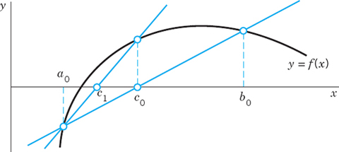
 - 24. Method of False Position (Regula falsi). Figure 430 shows the idea. We assume that f is continuous. We compute the x-intercept c0 of the line through (a0, f(a0)), (b0, f(b0)). If f(c0) = 0, we are done. If f(a0)f(c0) < 0 (as in Fig. 430), we set a1 = a0, b1 = c0 and repeat to get c1, etc. If f(a0)f(c0) > 0, then f(c0)f(b0) < 0 and we set a1 = c0, b1 = b0, etc.
(a) Algorithm. Show that

and write an algorithm for the method.
Fig. 430. Method of false position
(b) Solve x4 = 2,
 and x + ln x = 2, with a = 1, b = 2.
 - 25. TEAM PROJECT. Bisection Method. This simple but slowly convergent method for finding a solution of f(x) = 0 with continuous f is based on the intermediate value theorem, which states that if a continuous function f has opposite signs at some x = a and x = b (> a), that is, either f(a) < 0, f(b) > 0 or f(a) > 0, f(b) < 0, then f must be 0 somewhere on [a, b]. The solution is found by repeated bisection of the interval and in each iteration picking that half which also satisfies that sign condition.
(a) Algorithm. Write an algorithm for the method.
(b) Comparison. Solve x = cos x by Newton's method and by bisection. Compare.
(c) Solve e−x = ln x and ex + x4 + x = 2 by bisection.
26–29 SECANT METHOD
Solve, using x0 and x1 as indicated:
- 26. e−x − tan x = 0, x0 = 1, x1 = 0.7
- 27. Prob. 21, x0 = 1.0, x1 = 2.0
- 28. x = cos x, x0 = 0.5, x1 = 1
- 29. sin x = cot x, x0 = 1, x1 = 0.5
- 30. WRITING PROJECT. Solution of Equations. Compare the methods in this section and problem set, discussing advantages and disadvantages in terms of examples of your own. No proofs, just motivations and ideas.
19.3 Interpolation
We are given the values of a function f(x) at different points x0, x1, …, xn. We want to find approximate values of the function f(x) for “new” x’s that lie between these points for which the function values are given. This process is called interpolation. The student should pay close attention to this section as interpolation forms the underlying foundation for both Secs. 19.4 and 19.5. Indeed, interpolation allows us to develop formulas for numeric integration and differentiation as shown in Sec. 19.5.
Continuing our discussion, we write these given values of a function f in the form
![]()
or as ordered pairs
![]()
Where do these given function values come from? They may come from a “mathematical” function, such as a logarithm or a Bessel function. More frequently, they may be measured or automatically recorded values of an “empirical” function, such as air resistance of a car or an airplane at different speeds. Other examples of functions that are “empirical” are the yield of a chemical process at different temperatures or the size of the U.S. population as it appears from censuses taken at 10-year intervals.
A standard idea in interpolation now is to find a polynomial pn(x) of degree n (or less) that assumes the given values; thus

We call this pn an interpolation polynomial and x0, …, xn the nodes. And if f(x) is a mathematical function, we call pn an approximation of f (or a polynomial approximation, because there are other kinds of approximations, as we shall see later). We use pn to get (approximate) values of f for x’s between x0 and xn (“interpolation”) or sometimes outside this interval x0 ![]() x
x ![]() xn (“extrapolation”).
xn (“extrapolation”).
Motivation. Polynomials are convenient to work with because we can readily differentiate and integrate them, again obtaining polynomials. Moreover, they approximate continuous functions with any desired accuracy. That is, for any continuous f(x) on an interval J: a ![]() x
x ![]() b and error bound β > 0, there is a polynomial pn(x) (of sufficiently high degree n) such that
b and error bound β > 0, there is a polynomial pn(x) (of sufficiently high degree n) such that
![]()
This is the famous Weierstrass approximation theorem (for a proof see Ref. [GenRef7], App. 1).
Existence and Uniqueness. Note that the interpolation polynomial pn satisfying (1) for given data exists and we shall give formulas for it below. Furthermore, pn is unique: Indeed, if another polynomial qn also satisfies qn(x0) = f0, …, qn(xn) = fn, then pn(x) − qn(x) = 0 at x0, …, xn, but a polynomial pn − qn of degree n (or less) with n + 1 roots must be identically zero, as we know from algebra; thus pn(x) = qn(x) for all x, which means uniqueness.
How Do We Find pn? We shall explain several standard methods that give us pn. By the uniqueness proof above, we know that, for given data, the different methods must give us the same polynomial. However, the polynomials may be expressed in different forms suitable for different purposes.
Lagrange Interpolation
Given (x0, f0), (x1, f1), …, (xn, fn) with arbitrarily spaced xj, Lagrange had the idea of multiplying each fj by a polynomial that is 1 at xj and 0 at the other n nodes and then taking the sum of these n + 1 polynomials. Clearly, this gives the unique interpolation polynomial of degree n or less. Beginning with the simplest case, let us see how this works.
Linear interpolation is interpolation by the straight line through (x0, f0), (x1, f1); see Fig. 431. Thus the linear Lagrange polynomial p1 is a sum p1 = L0f0 + L1f1 with L0 the linear polynomial that is 1 at x0 and 0 at x1; similarly, L1 is 0 at x0 and 1 at x1. Obviously,
![]()
This gives the linear Lagrange polynomial
![]()

Fig. 431. Linear Interpolation
EXAMPLE 1 Linear Lagrange Interpolation
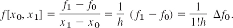
Compute a 4D-value of ln 9.2 from ln 9.0 = 2.1971, ln 9.5 = 2.2513 by linear Lagrange interpolation and determine the error, using ln 9.2 = 2.2192 (4D).
Solution.. x0 = 9.0, x1 = 9.5, f0 = ln 9.0, f1 = ln 9.5. Ln (2) we need
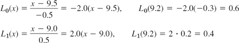
(see Fig. 432) and obtain the answer
![]()
The error is ![]() = a −
= a − ![]() = 2.2192 − 2.2188 = 0.0004. Hence linear interpolation is not sufficient here to get 4D accuracy; it would suffice for 3D accuracy.
= 2.2192 − 2.2188 = 0.0004. Hence linear interpolation is not sufficient here to get 4D accuracy; it would suffice for 3D accuracy.
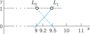
Fig. 432. L0 and L1 in Example 1
Quadratic interpolation is interpolation of given (x0, f0), (x1, f1), (x2, f2) by a second-degree polynomial p2(x), which by Lagrange's idea is
![]()
with L0(x0) = 1, L1(x1) = 1, L2(x2) = 1, and L0(x1) = L0(x2) = 0, etc. We claim that

How did we get this? Well, the numerator makes Lk(xj) = 0 if j ≠ k. And the denominator makes Lk(xk) = 1 because it equals the numerator at x = xk.
EXAMPLE 2 Quadratic Lagrange Interpolation
Compute ln 9.2 by (3) from the data in Example 1 and the additional third value ln 11.0 = 2.3979.
Solution. In (3),
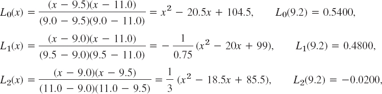
(see Fig. 433), so that (3a) gives, exact to 4D,
![]()
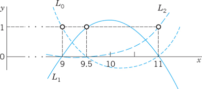
Fig. 433. L0, L1, L2 in Example 2
General Lagrange Interpolation Polynomial. For general n we obtain

where Lk(xk) = 1 and Lk is 0 at the other nodes, and the Lk are independent of the function f to be interpolated. We get (4a) if we take

We can easily see that pn(xk) = fk. Indeed, inspection of (4b) shows that lk(xj) = 0 if j ≠ k, so that for x = xk, the sum in (4a) reduces to the single term (lk(xk)/lk(xk))fk = fk.
Error Estimate. If f is itself a polynomial of degree n (or less), it must coincide with pn because the n + 1 data (x0, f0), …, (xn, fn) determine a polynomial uniquely, so the error is zero. Now the special f has its (n + 1)st derivative identically zero. This makes it plausible that for a general f its (n + 1)st derivative f(n + 1) should measure the error
![]()
It can be shown that this is true if f(n + 1) exists and is continuous. Then, with a suitable t between x0 and xn (or between x0, xn, and x if we extrapolate),

Thus |![]() n(x)| is 0 at the nodes and small near them, because of continuity. The product (x − x0)…(x − xn) is large for x away from the nodes. This makes extrapolation risky. And interpolation at an x will be best if we choose nodes on both sides of that x. Also, we get error bounds by taking the smallest and the largest value of f(n + 1)(t) in (5) on the interval x0
n(x)| is 0 at the nodes and small near them, because of continuity. The product (x − x0)…(x − xn) is large for x away from the nodes. This makes extrapolation risky. And interpolation at an x will be best if we choose nodes on both sides of that x. Also, we get error bounds by taking the smallest and the largest value of f(n + 1)(t) in (5) on the interval x0 ![]() t
t ![]() xn (or on the interval also containing x if we extrapolate).
xn (or on the interval also containing x if we extrapolate).
Most importantly, since pn is unique, as we have shown, we have
THEOREM 1 Error of Interpolation
Formula (5) gives the error for any polynomial interpolation method if f(x) has a continuous (n + 1)st derivative.
Practical error estimate. If the derivative in (5) is difficult or impossible to obtain, apply the Error Principle (Sec. 19.1), that is, take another node and the Lagrange polynomial pn + 1(x) and regard pn + 1(x) − pn(x) as a (crude) error estimate for pn(x).
EXAMPLE 3 Error Estimate (5) of Linear Interpolation. Damage by Roundoff. Error Principle
Estimate the error in Example 1 first by (5) directly and then by the Error Principle (Sec. 19.1).
Solution. (A) Estimation by(5). We have n = 1, f(t) = ln t, f′(t) = 1/t, f″(t) = −1/t2. Hence

t = 0.9 gives the maximum 0.03/92 = 0.00037 and t = 9.5 gives the minimum 0.03/9.52 = 0.00033, so that we get 0.00033 ![]()
![]() 1 (9.2)
1 (9.2) ![]() 0.00037, or better, 0.00038 because 0.3/81 = 0.003703 ….
0.00037, or better, 0.00038 because 0.3/81 = 0.003703 ….
But the error 0.0004 in Example 1 disagrees, and we can learn something! Repetition of the computation there with 5D instead of 4D gives
![]()
with an actual error ![]() = 2.21920 − 2.21885 = 0.00035, which lies nicely near the middle between our two error bounds.
= 2.21920 − 2.21885 = 0.00035, which lies nicely near the middle between our two error bounds.
This shows that the discrepancy (0.0004 vs. 0.00035) was caused by rounding, which is not taken into account in (5).
(B) Estimation by the Error Principle. We calculate p1(9.2) = 2.21885 as before and then p2(9.2) as in Example 2 but with 5D, obtaining
![]()
The difference p2(9.2) − p1(9.2) = 0.00031 is the approximate error of p1(9.2) that we wanted to obtain; this is an approximation of the actual error 0.00035 given above.
Newton's Divided Difference Interpolation
For given data (x0, f0), …, (xn, fn) the interpolation polynomial pn(x) satisfying (1) is unique, as we have shown. But for different purposes we may use pn(x) in different forms. Lagrange's form just discussed is useful for deriving formulas in numeric differentiation (approximation formulas for derivatives) and integration (Sec. 19.5).
Practically more important are Newton's forms of pn(x), which we shall also use for solving ODEs (in Sec. 21.2). They involve fewer arithmetic operations than Lagrange's form. Moreover, it often happens that we have to increase the degree n to reach a required accuracy. Then in Newton's forms we can use all the previous work and just add another term, a possibility without counterpart for Lagrange's form. This also simplifies the application of the Error Principle (used in Example 3 for Lagrange). The details of these ideas are as follows.
Let pn−1(x) be the (n − 1)st Newton polynomial (whose form we shall determine); thus pn−1(x0) = f0, pn−1(x1) = f1, …, pn−1(xn−1) = fn−1. Furthermore, let us write the nth Newton polynomial as
![]()
![]()
Here gn(x) is to be determined so that pn(x0) = f0, pn(x1) = f1, …, pn(xn) = fn.
Since pn and pn−1 agree at x0, …, xn−1, we see that gn is zero there. Also, gn will generally be a polynomial of nth degree because so is pn, whereas pn−1 can be of degree n − 1 at most. Hence gn must be of the form
![]()
We determine the constant an. For this we set x = xn and solve (6″) algebraically for an. Replacing gn(xn) according to (6′) and using pn(xn) = fn, we see that this gives

We write ak instead of an and show that ak equals the kth divided difference, recursively denoted and defined as follows:

and in general

If n = 1, then pn−1(xn) = p0(x1) = f0 because p0(x) is constant and equal to f0, the value of f(x) at x0. Hence (7) gives
![]()
and (6) and (6″) give the Newton interpolation polynomial of the first degree
![]()
If n = 2, then this p1 and (7) give

where the last equality follows by straightforward calculation and comparison with the definition of the right side. (Verify it; be patient.) From (6) and (6″) we thus obtain the second Newton polynomial
For n = k, formula (6) gives
![]()
With p0(x) = f0 by repeated application with k = 1, …, n this finally gives Newton's divided difference interpolation formula

An algorithm is shown in Table 19.2. The first do-loop computes the divided differences and the second the desired value ![]()
Example 4 shows how to arrange differences near the values from which they are obtained; the latter always stand a half-line above and a half-line below in the preceding column. Such an arrangement is called a (divided) difference table.
Table 19.2 Newton's Divided Difference Interpolation

EXAMPLE 4 Newton's Divided Difference Interpolation Formula
Compute f(9.2) from the values shown in the first two columns of the following table.

Solution. We compute the divided differences as shown. Sample computation:
![]()
The values we need in (10) are circled. We have

At x = 9.2,
![]()
The value exact to 6D is f(9.2) = ln 9.2 = 2.219203. Note that we can nicely see how the accuracy increases from term to term:
![]()
Equal Spacing: Newton's Forward Difference Formula
Newton's formula (10) is valid for arbitrarily spaced nodes as they may occur in practice in experiments or observations. However, in many applications the xj’s are regularly spaced—for instance, in measurements taken at regular intervals of time. Then, denoting the distance by h, we can write

We show how (8) and (10) now simplify considerably!
To get started, let us define the first forward difference of f at xj by
![]()
the second forward difference of f at xj by
![]()
and, continuing in this way, the kth forward difference of f at xj by

Examples and an explanation of the name “forward” follow on the next page. What is the point of this? We show that if we have regular spacing (11), then

PROOF
We prove (13) by induction. It is true for k = 1 because x1 = x0 + h, so that
Assuming (13) to be true for all forward differences of order k, we show that (13) holds for k + 1. We use (8) with k + 1 instead of k; then we use (k + 1)h = xk+1 − x0, resulting from (11), and finally (12) with j = 0, that is, Δk+1f0 = Δkf1 − Δkf0. This gives

which is (13) with k + 1 instead of k. Formula (13) is proved.
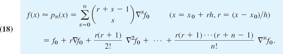
In (10) we finally set x = x0 + rh. Then x − x0 = rh, x − x1 = (r − 1)h since x1 − x0 = h, and so on. With this and (13), formula (10) becomes Newton's (or Gregory2–Newton's) forward difference interpolation formula
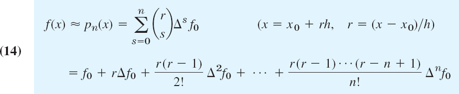
where the binomial coefficients in the first line are defined by

and s! = 1 · 2 … s.
Error. From (5) we get, with x − x0 = rh, x − x1 = (r − 1)h, etc.,

with t as characterized in (5).
Formula (16) is an exact formula for the error, but it involves the unknown t. In Example 5 (below) we show how to use (16) for obtaining an error estimate and an interval in which the true value of f(x) must lie.
Comments on Accuracy. (A) The order of magnitude of the error ![]() n(x) is about equal to that of the next difference not used in pn(x).
n(x) is about equal to that of the next difference not used in pn(x).
(B) One should choose x0, …, xn such that the x at which one interpolates is as well centered between x0, …, xn as possible.
The reason for (A) is that in (16),

(and actually for any r as long as we do not extrapolate). The reason for (B) is that |r(r − 1) … (r − n)| becomes smallest for that choice.
EXAMPLE 5 Newton's Forward Difference Formula. Error Estimation
Compute cosh 0.56 from (14) and the four values in the following table and estimate the error.

Solution. We compute the forward differences as shown in the table. The values we need are circled. In (14) we have r = (0.56 − 0.50)/0.1 = 0.6 so that (14) gives

Error estimate. From (16), since the fourth derivative is cosh(4)t = cosh t,
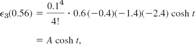
where A = −0.00000336 and 0.5 ![]() t
t ![]() 0.8. We do not know t, but we get an inequality by taking the largest and smallest cosh t in that interval:
0.8. We do not know t, but we get an inequality by taking the largest and smallest cosh t in that interval:
![]()
Since
![]()
![]()
Numeric values are
![]()
The exact 6D-value is cosh 0.56 = 1.160941. It lies within these bounds. Such bounds are not always so tight. Also, we did not consider roundoff errors, which will depend on the number of operations.
This example also explains the name “forward difference formula”: we see that the differences in the formula slope forward in the difference table.
Equal Spacing: Newton's Backward Difference Formula
Instead of forward-sloping differences we may also employ backward-sloping differences. The difference table remains the same as before (same numbers, in the same positions), except for a very harmless change of the running subscript j (which we explain in Example 6, below). Nevertheless, purely for reasons of convenience it is standard to introduce a second name and notation for differences as follows. We define the first backward difference of f at xj by
![]()
the second backward difference of f at xj by
![]()
and, continuing in this way, the kth backward difference of f at xj by

A formula similar to (14) but involving backward differences is Newton's (or Gregory–Newton's) backward difference interpolation formula
EXAMPLE 6 Newton's Forward and Backward Interpolations
Compute a 7D-value of the Bessel function J0(x) for x = 1.72 from the four values in the following table, using (a) Newton's forward formula (14), (b) Newton's backward formula (18).

Solution. The computation of the differences is the same in both cases. Only their notation differs.
(a) Forward. In (14) we have r = (1.72 − 1.70)/0.1 = 0.2, and j goes from 0 to 3 (see first column). In each column we need the first given number, and (14) thus gives

which is exact to 6D, the exact 7D-value being 0.3864185.
(b) Backward. For (18) we use j shown in the second column, and in each column the last number. Since r = (1.72 − 200)/0.1 = −2.8, we thus get from (18)

There is a third notation for differences, called the central difference notation. It is used in numerics for ODEs and certain interpolation formulas. See Ref. [E5] listed in App. 1.
- Linear interpolation. Calculate p1(x) in Example 1 and from it ln 9.3.
- Error estimate. Estimate the error in Prob. 1 by (5).
- Quadratic interpolation. Gamma function. Calculate the Lagrange polynomial p2(x) for the values Γ (1.00) = 1.0000, Γ (1.02) = 0.9888, Γ (1.04) = 0.9784 of the gamma function [(24) in App. A3.1] and from it approximations of Γ (1.01) and Γ (1.03)
- Error estimate for quadratic interpolation. Estimate the error for p2(9.2) in Example 2 from (5).
- Linear and quadratic interpolation. Find e−0.25 and e−0.75 by linear interpolation of e−x with x0 = 0, x1 = 0.5 and x0 = 0.5, x1 = 1, respectively. Then find p2(x) by quadratic interpolation of e−x with x0 = 0, x1 = 0.5, x2 = 1 and from it e−0.25 and e−0.75 Compare the errors. Use 4S-values of e−x.
- Interpolation and extrapolation. Calculate p2(x) in Example 2. Compute from it approximations of ln 9.4, ln 10, ln 10.5, ln 11.5, and ln 12. Compute the errors by using exact 5S-values and comment.
- Interpolation and extrapolation. Find the quadratic polynomial that agrees with sin x at x = 0, π/4, π/2 and use it for the interpolation and extrapolation of sin x at x = −π/8, π/8, 3π/8, 5π/8. Compute the errors.
- Extrapolation. Does a sketch of the product of the (x − xj) in (5) for the data in Example 2 indicate that extrapolation is likely to involve larger errors than interpolation does?
- Error function (35) in App. A3.1. Calculate the Lagrange polynomial p2(x) for the 5S-values f(0.25) = 0.27633, f(0.5) = 0.52050, f(1.0) = 0.84270 and from p2(x) an approximation of f(0.75) (= 0.71116).
- Error bound. Derive an error bound in Prob. 9 from (5).
- Cubic Lagrange interpolation. Bessel function J0. Calculate and graph L0, L1, L2, L3 with x0 = 0, x1 = 1, x2 = 2, x3 = 3 on common axes. Find p3(x) for the data (0, 1), (1, 0.765198), (2, 0.223891), (3, −0.260052) [values of the Bessel function J0(f)]. Find p3 for x = 0.5, 1.5, 2.5 and compare with the 6S-exact values 0.938470, 0.511828, −0.048384.
- Newton's forward formula (14). Sine integral. Using (14), find f(1.25) by linear, quadratic, and cubic interpolation of the data (values of (40) in App. A31); 6S-value Si(1.25) = 1.14645)f(1.0) = 0.94608, f(1.5) = 1.32468, f(2.0) = 1.60541, f(2.5) = 1.77852, and compute the errors. For the linear interpolation f(1.0) use f(1.5) for the quadratic f(1.0), f(1.5), f(2.0) etc.
- Lower degree. Find the degree of the interpolation polynomial for the data (−4, 50), (−2, 18), (0,2), (2,2), (4, 18), using a difference table. Find the polynomial.
- Newton's forward formula (14). Gamma function. Set up (14) for the data in Prob. 3 and compute Γ (1.01), Γ (1.03), Γ (1.05).
- Divided differences. Obtain p2 in Example 2 from (10).
- Divided differences. Error function. Compute p2(0.75) from the data in Prob. 9 and Newton's divided difference formula (10).
- Backward difference formula (18). Use p2(x) in (18) and the values of erf x, x = 0.2, 0.4, 0.6 in Table A4 of App. 5, compute erf 0.3 and the error. (4S-exact erg 0.3 = 0.3286).
- In Example 5 of the text, write down the difference table as needed for (18), then write (18) with general x and then with x = 0.56 to verify the answer in Example 5.
- CAS EXPERIMENT. Adding Terms in Newton Formulas. Write a program for the forward formula (14). Experiment on the increase of accuracy by successively adding terms. As data use values of some function of your choice for which your CAS gives the values needed in determining errors.
- TEAM PROJECT. Interpolation and Extrapolation. (a) Lagrange practical error estimate (after Theorem 1). Apply this to p1(9.2) and p2(9.2) for the data x0 = 9.0, x1 = 9.5, x2 = 11.0, f0 = ln x0, f1 = ln x1, f2 = ln x2 (6S-values).
(b) Extrapolation. Given (xj, f(xj)) = (0.2, 0.9980), (0.4, 0.9686), (0.6, 0.8443), (0.8, 0.5358), (1.0, 0). Find f(0.7) from the quadratic interpolation polynomials based on (α) 0.6, 0.8, 1.0, (β) 0.4, 0.6, 0.8, (γ) 0.2, 0.4, 0.6. Compare the errors and comment. [Exact f(x) =
 f(0.7) = 0.7181 (4S).]
(c) Graph the product of factors (x − xj) in the error formula (5) for n = 2, …, 10 separately. What do these graphs show regarding accuracy of interpolation and extrapolation?
- WRITING PROJECT. Comparison of interpolation methods. List 4–5 ideas that you feel are most important in this section. Arrange them in best logical order. Discuss them in a 2–3 page report.
19.4 Spline Interpolation
Given data (function values, points in the xy-plane) (x0, f0), (x1, f1), …, (xn, fn) can be interpolated by a polynomial pn(x) of degree n or less so that the curve of pn(x) passes through these n + 1 points (xj, fj); here f0 = f(x0), …, fn = f(xn), See Sec. 19.3.
Now if n is large, there may be trouble: pn(x) may tend to oscillate for x between the nodes x0, …, xn. Hence we must be prepared for numeric instability (Sec. 19.1). Figure 434 shows a famous example by C. Runge3 for which the maximum error even approaches ∞ as n → ∞ (with the nodes kept equidistant and their number increased). Figure 435 illustrates the increase of the oscillation with n for some other function that is piecewise linear.
Those undesirable oscillations are avoided by the method of splines initiated by I. J. Schoenberg in 1946 (Quarterly of Applied Mathematics 4, pp. 45–99, 112–141). This method is widely used in practice. It also laid the foundation for much of modern CAD (computer-aided design). Its name is borrowed from a draftman's spline, which is an elastic rod bent to pass through given points and held in place by weights. The mathematical idea of the method is as follows:

Fig. 434. Runge's example f(x) = 1/(1 +x2) and interpolating polynomial P10(x)

Fig. 435. Piecewise linear function f(x) and interpolation polynomials of increasing degrees
Instead of using a single high-degree polynomial Pn over the entire interval a ![]() x
x ![]() b in which the nodes lie, that is,
b in which the nodes lie, that is,
![]()
we use n low-degree, e.g., cubic, polynomials
![]()
one over each subinterval between adjacent nodes, hence q0 from x0 to x1, then q1 from x1 to x2, and so on. From this we compose an interpolation function g(x), called a spline, by fitting these polynomials together into a single continuous curve passing through the data points, that is,
![]()
Note that g(x) = q0(x) when x0 ![]() x
x ![]() x1, then g(x) = q1(x) when x1
x1, then g(x) = q1(x) when x1 ![]() x
x ![]() x2, and so on, according to our construction of g.
x2, and so on, according to our construction of g.
Thus spline interpolation is piecewise polynomial interpolation.
The simplest qj’s would be linear polynomials. However, the curve of a piecewise linear continuous function has corners and would be of little interest in general—think of designing the body of a car or a ship.
We shall consider cubic splines because these are the most important ones in applications. By definition, a cubic spline g(x) interpolating given data (x0, f0), …, (xn, fn) is a continuous function on the interval a = x0 ![]() x
x ![]() xn = b that has continuous first and second derivatives and satisfies the interpolation condition (2); furthermore, between adjacent nodes, g(x) is given by a polynomial qj(x) of degree 3 or less.
xn = b that has continuous first and second derivatives and satisfies the interpolation condition (2); furthermore, between adjacent nodes, g(x) is given by a polynomial qj(x) of degree 3 or less.
We claim that there is such a cubic spline. And if in addition to (2) we also require that
![]()
(given tangent directions of g(x) at the two endpoints of the interval a ![]() x
x ![]() b), then we have a uniquely determined cubic spline. This is the content of the following existence and uniqueness theorem, whose proof will also suggest the actual determination of splines. (Condition (3) will be discussed after the proof.)
b), then we have a uniquely determined cubic spline. This is the content of the following existence and uniqueness theorem, whose proof will also suggest the actual determination of splines. (Condition (3) will be discussed after the proof.)
THEOREM 1 Existence and Uniqueness of Cubic Splines
Let (x0, f0), (x1, f1), …, (xn, fn) with given (arbitrarily spaced) xj [see (1)] and given fj = f(xj), j = 0, 1, …, n. Let k0 and kn be any given numbers. Then there is one and only one cubic spline g(x) corresponding to (1) and satisfying (2) and (3).
PROOF
By definition, on every subinterval Ij given by xj ![]() x
x ![]() xj+1, the spline g(x) must agree with a polynomial qj(x) of degree not exceeding 3 such that
xj+1, the spline g(x) must agree with a polynomial qj(x) of degree not exceeding 3 such that
![]()
For the derivatives we write
![]()
with k0 and kn given and k1, …, kn−1 to be determined later. Equations (4) and (5) are four conditions for each qj(x). By direct calculation, using the notation

we can verify that the unique cubic polynomial qj(x) (j = 0, 1, …, n − 1) satisfying (4) and (5) is

Differentiating twice, we obtain
![]()
![]()
By definition, g(x) has continuous second derivatives. This gives the conditions
![]()
If we use (8) with j replaced by j − 1, and (7), these n − 1 equations become

where ∇fj = f(xj) − f(xj−1) and ∇fj+1 = f(xj+1) − f(xj) and j = 1, …, n − 1, as before. This linear system of n − 1 equations has a unique solution k1, …, kn−1 since the coefficient matrix is strictly diagonally dominant (that is, in each row the (positive) diagonal entry is greater than the sum of the other (positive) entries). Hence the determinant of the matrix cannot be zero (as follows from Theorem 3 in Sec. 20.7), so that we may determine unique values k1, …, kn−1 of the first derivative of g(x) at the nodes. This proves the theorem.
Storage and Time Demands in solving (9) are modest, since the matrix of (9) is sparse (has few nonzero entries) and tridiagonal (may have nonzero entries only on the diagonal and on the two adjacent “parallels” above and below it). Pivoting (Sec. 7.3) is not necessary because of that dominance. This makes splines efficient in solving large problems with thousands of nodes or more. For some literature and some critical comments, see American Mathematical Monthly 105 (1998), 929–941.
Condition (3) includes the clamped conditions
![]()
in which the tangent directions f′(x0) and f′(xn) at the ends are given. Other conditions of practical interest are the free or natural conditions
![]()
(geometrically: zero curvature at the ends, as for the draftman's spline), giving a natural spline. These names are motivated by Fig. 293 in Problem Set 12.3.
Determination of Splines. Let k0 and kn be given. Obtain k1, …, kn−1 by solving the linear system (9). Recall that the spline g(x) to be found consists of n cubic polynomials q0, …, qn−1. We write these polynomials in the form

where j = 0, …, n − 1. Using Taylor's formula, we obtain
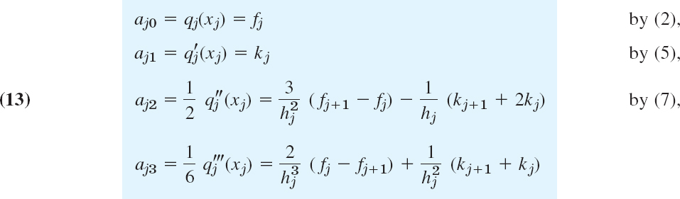
with aj3 obtained by calculating ![]() from (12) and equating the result to (8), that is,
from (12) and equating the result to (8), that is,

and now subtracting from this 2aj2 as given in (13) and simplifying.
Note that for equidistant nodes of distance hj = h we can write cj = c = 1/j in (6*) and have from (9) simply

EXAMPLE 1 Spline Interpolation. Equidistant Nodes
Interpolate f(x) = x4 on the interval −1 ![]() x
x ![]() x
x ![]() 1 by the cubic spline g(x) corresponding to the nodes x0 = −1, x1 = 0, x2 = 1 and satisfying the clamped conditions g′(−1) = f′(−1), g′(1) = f′(1).
1 by the cubic spline g(x) corresponding to the nodes x0 = −1, x1 = 0, x2 = 1 and satisfying the clamped conditions g′(−1) = f′(−1), g′(1) = f′(1).
Solution. In our standard notation the given data are f0 = f(−1) = 1, f1 = f(0) = 0, f2 = f(1) = 1. We have h = 1 and n = 2, so that our spline consists of n = 2 polynomials

We determine the kj from (14) (equidistance!) and then the coefficients of the spline from (13). Since n = 2, the system (14) is a single equation (with j = 1 and h = 1)
![]()
Here f0 = f2 = 1 (the value of x4 at the ends) and k0 = −4, k2 = 4, the values of the derivative 4x3 at the ends −1 and 1. Hence
![]()
From (13) we can now obtain the coefficients of q0, namely, a00 = f0 = 1, a01 = k0 = −4, and
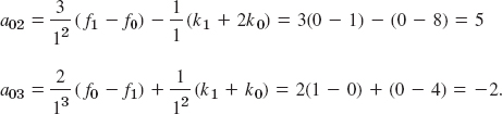
Similarly, for the coefficients of q1 we obtain from (13) the values a10 = f1 = 0, a11 = k1 = 0, and

This gives the polynomials of which the spline g(x) consists, namely,

Figure 436 shows f(x) and this spline. Do you see that we could have saved over half of our work by using symmetry?

Fig. 436. Function f(x) = x4 and cubic spline g(x) in Example 1
EXAMPLE 2 Natural Spline. Arbitrarily Spaced Nodes
Find a spline approximation and a polynomial approximation for the curve of the cross section of the circular-shaped Shrine of the Book in Jerusalem shown in Fig. 437.
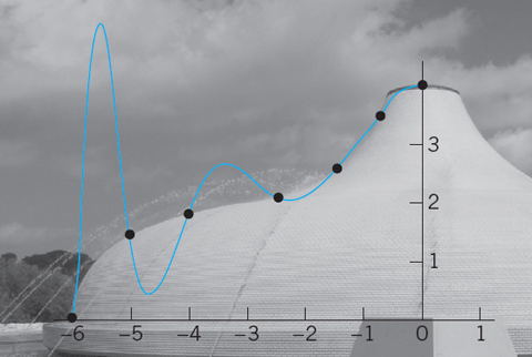
Fig. 437. Shrine of the Book in Jerusalem (Architects F. Kissler and A. M. Bartus)
Solution. Thirteen points, about equally distributed along the contour (not along the x-axis!), give these data:

The figure shows the corresponding interpolation polynomial of 12th degree, which is useless because of its oscillation. (Because of roundoff your software will also give you small error terms involving odd powers of x.) The polynomial is

The spline follows practically the contour of the roof, with a small error near the nodes −0.8 and 0.8. The spline is symmetric. Its six polynomials corresponding to positive x have the following coefficients of their representations (12). (Note well that (12) is in terms of powers of, x − xj not x!)

- WRITING PROJECT. Splines. In your own words, and using as few formulas as possible, write a short report on spline interpolation, its motivation, a comparison with polynomial interpolation, and its applications.
2–9 VERIFICATIONS. DERIVATIONS. COMPARISONS
- 2. Individual polynomial qj. Show that qj(x) in (6) satisfies the interpolation condition (4) as well as the derivative condition (5).
- 3. Verify the differentiations that give (7) and (8) from (6).
- 4. System for derivatives. Derive the basic linear system (9) for k1, …, kn−1 as indicated in the text.
- 5. Equidistant nodes. Derive (14) from (9).
- 6. Coefficients. Give the details of the derivation of aj2 and aj3 in (13).
- 7. Verify the computations in Example 1.
- 8. Comparison. Compare the spline g in Example 1 with the quadratic interpolation polynomial over the whole interval. Find the maximum deviations of g and p2 from f. Comment.
- 9. Natural spline condition. Using the given coefficients, verify that the spline in Example 2 satisfies g″(x) = 0 at the ends.
10–16 DETERMINATION OF SPLINES
Find the cubic spline g(x) for the given data with k0 and kn as given.
- 10. f(−2) = f(−1) = f(1) = f(2) = 0, f(0) = 1, k0 = k4 = 0
- 11. If we started from the piecewise linear function in Fig. 438, we would obtain g(x) in Prob. 10 as the spline satisfying g′(−2) = f′(−2) = 0, g′(2) = f′(2) = 0. Find and sketch or graph the corresponding interpolation polynomial of 4th degree and compare it with the spline. Comment.

Fig. 438. Spline and interpolation polynomial in Probs. 10 and 11
- 12.
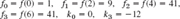
- 13.
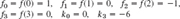
- 14.

- 15.

- 16.
 Can you obtain the answer from that of Prob. 15?
 - 17. If a cubic spline is three times continuously differentiable (that is, it has continuous first, second, and third derivatives), show that it must be a single polynomial.
- 18. CAS EXPERIMENT. Spline versus Polynomial. If your CAS gives natural splines, find the natural splines when x is integer from −m to m, and y(0) = 1 and all other y equal to 0. Graph each such spline along with the interpolation polynomial p2m. Do this for m = 2 to 10 (or more). What happens with increasing m?
- 19. Natural conditions. Explain the remark after (11).
- 20. TEAM PROJECT. Hermite Interpolation and Bezier Curves. In Hermite interpolation we are looking for a polynomial p(x) (of degree 2n + 1 or less) such that and its derivative p′(x) have given values at n + 1 nodes. (More generally, p(x), p′(x), p″(x), … may be required to have given values at the nodes.)
(a) Curves with given endpoints and tangents. Let C be a curve in the xy-plane parametrically represented by r(t) = [x(t), y(t)], 0
t 1 (see Sec. 9.5). Show that for given initial and terminal points of a curve and given initial and terminal tangents, say,
we can find a curve C, namely,


Note that this is a cubic Hermite interpolation polynomial, and n = 1 because we have two nodes (the endpoints of C). (This has nothing to do with the Hermite polynomials in Sec. 5.8.) The two points

and

are called guidepoints because the segments AGA and BGB specify the tangents graphically. A, B, GA, GB determine C, and C can be changed quickly by moving the points. A curve consisting of such Hermite interpolation polynomials is called a Bezier curve, after the French engineer P. Bezier of the Renault Automobile Company, who introduced them in the early 1960s in designing car bodies. Bezier curves (and surfaces) are used in computer-aided design (CAD) and computer-aided manufacturing (CAM). (For more details, see Ref. [E21] in App. 1.)
(b) Find and graph the Bezier curve and its guidepoints if A: [0, 0], B: [1, 0],


(c) Changing guidepoints changes C. Moving guidepoints farther away results in C “staying near the tangents for a longer time.” Confirm this by changing v0 and v1 in (b) to 2v0 and 2v1 (see Fig. 439).
(d) Make experiments of your own. What happens if you change v1 in (b) to −v1. If you rotate the tangents? If you multiply v0 and v1 by positive factors less than 1?

19.5 Numeric Integration and Differentiation
In applications, the engineer often encounters integrals that are very difficult or even impossible to solve analytically. For example, the error function, the Fresnel integrals (see Probs. 16–25 on nonelementary integrals in this section), and others cannot be evaluated by the usual methods of calculus (see App. 3, (24)–(44) for such “difficult” integrals). We then need methods from numerical analysis to evaluate such integrals. We also need numerics when the integrand of the integral to be evaluated consists of an empirical function, where we are given some recorded values of that function. Methods that address these kinds of problems are called methods of numeric integration.
Numeric integration means the numeric evaluation of integrals

where a and b are given and f is a function given analytically by a formula or empirically by a table of values. Geometrically, J is the area under the curve of f between a and b (Fig. 440), taken with a minus sign where f is negative.
We know that if f is such that we can find a differentiable function F whose derivative is f, then we can evaluate J directly, i.e., without resorting to numeric integration, by applying the familiar formula

Your CAS (Mathematica, Maple, etc.) or tables of integrals may be helpful for this purpose.
Rectangular Rule. Trapezoidal Rule
Numeric integration methods are obtained by approximating the integrand f by functions that can easily be integrated.
The simplest formula, the rectangular rule, is obtained if we subdivide the interval of integration a ![]() x
x ![]() b into n subintervals of equal length h = (b − a)/n and in each subinterval approximate f by the constant
b into n subintervals of equal length h = (b − a)/n and in each subinterval approximate f by the constant ![]() the value of f at the midpoint
the value of f at the midpoint ![]() of the jth subinterval (Fig. 441). Then f is approximated by a step function (piecewise constant function), the n rectangles in Fig. 441 have the areas
of the jth subinterval (Fig. 441). Then f is approximated by a step function (piecewise constant function), the n rectangles in Fig. 441 have the areas ![]() and the rectangular rule is
and the rectangular rule is

The trapezoidal rule is generally more accurate. We obtain it if we take the same subdivision as before and approximate f by a broken line of segments (chords) with endpoints [a, f(a)], [x1, f(x1)], …, [b, f(b)] on the curve of f (Fig. 442). Then the area under the curve of f between a and b is approximated by n trapezoids of areas
![]()
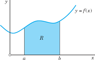
Fig. 440. Geometric interpretation of a definite integral


By taking their sum we obtain the trapezoidal rule

where h = (b − a)/n, as in (1). The xj’s and a and b are called nodes.
Evaluate ![]() by means of (2) with n = 10.
by means of (2) with n = 10.
Note that this integral cannot be evaluated by elementary calculus, but leads to the error function (see Eq. (35), App. 3).
Solution. J ≈ 0.1(0.5 · 1.367879 + 6.778167) = 0.746211 from Table 19.3.
Table 19.3 Computations in Example 1
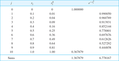
Error Bounds and Estimate for the Trapezoidal Rule
An error estimate for the trapezoidal rule can be derived from (5) in Sec. 19.3 with n = 1 by integration as follows. For a single subinterval we have
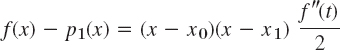
with a suitable t depending on x, between x0 and x1. Integration over x from a = x0 to x1 = x0 + h gives

Setting x − x0 = v and applying the mean value theorem of integral calculus, which we can use because (x − x0)(x − x0 − h) does not change sign, we find that the right side equals
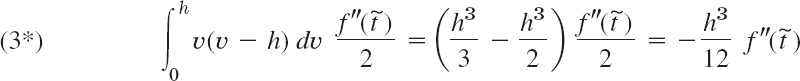
where ![]() is a (suitable, unknown) value between x0 and x1. This is the error for the trapezoidal rule with n = 1, often called the local error.
is a (suitable, unknown) value between x0 and x1. This is the error for the trapezoidal rule with n = 1, often called the local error.
Hence the error ![]() of (2) with any n is the sum of such contributions from the n subintervals; since h = (b − a)/n, nh3 = n(b − a)3/n3, and (b − a)2 = n2h2, we obtain
of (2) with any n is the sum of such contributions from the n subintervals; since h = (b − a)/n, nh3 = n(b − a)3/n3, and (b − a)2 = n2h2, we obtain
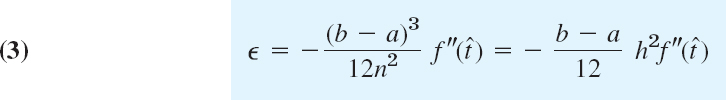
with (suitable, unknown) ![]() between a and b.
between a and b.
Because of (3) the trapezoidal rule (2) is also written

Error Bounds are now obtained by taking the largest value for f″, say, M2, and the smallest value, ![]() in the interval of integration. Then (3) gives (note that K is negative)
in the interval of integration. Then (3) gives (note that K is negative)

Error Estimation by Halving h is advisable if f″ is very complicated or unknown, for instance, in the case of experimental data. Then we may apply the Error Principle of Sec. 19.1. That is, we calculate by (2), first with h, obtaining, say, J = Jh + ![]() h, and then with
h, and then with ![]() obtaining J = Jh/2 +
obtaining J = Jh/2 + ![]() h/2. Now if we replace h2 in (3) with
h/2. Now if we replace h2 in (3) with ![]() the error is multiplied by
the error is multiplied by ![]() . Hence
. Hence ![]() (not exactly because
(not exactly because ![]() may differ). Together, Jh/2 +
may differ). Together, Jh/2 + ![]() h/2 = Jh +
h/2 = Jh + ![]() h ≈ Jh + 4
h ≈ Jh + 4![]() h/2. Thus Jh/2 − Jh = (4 − 1)
h/2. Thus Jh/2 − Jh = (4 − 1)![]() h/2. Division by 3 gives the error formula for Jh/2
h/2. Division by 3 gives the error formula for Jh/2

EXAMPLE 2 Error Estimation for the Trapezoidal Rule by (4) and (5)
Estimate the error of the approximate value in Example 1 by (4) and (5).
Solution. (A) Error bounds by (4). By differentiation, ![]() Also, f″′(x) > 0 if 0 < x < 1, so that the minimum and maximum occur at the ends of the interval. We compute M2 = f″(1) = 0.735759 and
Also, f″′(x) > 0 if 0 < x < 1, so that the minimum and maximum occur at the ends of the interval. We compute M2 = f″(1) = 0.735759 and ![]() Furthermore, k = −1/1200, and (4) gives
Furthermore, k = −1/1200, and (4) gives
![]()
Hence the exact value of J must lie between
![]()
Actually, J = 0.746824, exact to 6D.
(B) Error estimate by (5). Jn = 0.746211 in Example 1. Also,

Hence ![]() and Jh/2 +
and Jh/2 + ![]() h/2 = 0.746824, exact to 6D.
h/2 = 0.746824, exact to 6D.
Simpson's Rule of Integration
Piecewise constant approximation of f led to the rectangular rule (1), piecewise linear approximation to the trapezoidal rule (2), and piecewise quadratic approximation will lead to Simpson's rule, which is of great practical importance because it is sufficiently accurate for most problems, but still sufficiently simple.
To derive Simpson's rule, we divide the interval of integration a ![]() x
x ![]() b into an even number of equal subintervals, say, into n = 2m subintervals of length h = (b − a)/(2m), with endpoints x0(= a), x1, …, x2m−1, x2m (= b); see Fig. 443. We now take the first two subintervals and approximate f(x) in the interval x0
b into an even number of equal subintervals, say, into n = 2m subintervals of length h = (b − a)/(2m), with endpoints x0(= a), x1, …, x2m−1, x2m (= b); see Fig. 443. We now take the first two subintervals and approximate f(x) in the interval x0 ![]() x
x ![]() x2 = x0 + 2h by the Lagrange polynomial p2(x) through (x0, f0), (x1, f1), (x2, f2), where fj = f(xj). From (3) in Sec. 19.3 we obtain
x2 = x0 + 2h by the Lagrange polynomial p2(x) through (x0, f0), (x1, f1), (x2, f2), where fj = f(xj). From (3) in Sec. 19.3 we obtain

The denominators in (6) are 2h2, −h2, and 2h2, respectively. Setting s = (x − x1)/h, we have

and we obtain
![]()
We now integrate with respect to x from x0 to x2. This corresponds to integrating with respect to s from −1 to 1. Since dx = h ds, the result is


A similar formula holds for the next two subintervals from x2 to x4, and so on. By summing all these m formulas we obtain Simpson's rule4

where h = (b − a)/(2m) and fj = f(xj). Table 19.4 shows an algorithm for Simpson's rule.
Table 19.4 Simpson's Rule of Integration

Error of Simpson's Rule (7). If the fourth derivative f(4) exists and is continuous on a ![]() x
x ![]() b, the error of (7), call it
b, the error of (7), call it ![]() s, is
s, is

here ![]() is a suitable unknown value between a and b. This is obtained similarly to (3). With this we may also write Simpson's rule (7) as
is a suitable unknown value between a and b. This is obtained similarly to (3). With this we may also write Simpson's rule (7) as

Error Bounds. By taking for f(4) in (8) the maximum M4 and minimum ![]() on the interval of integration we obtain from (8) the error bounds (note that C is negative)
on the interval of integration we obtain from (8) the error bounds (note that C is negative)
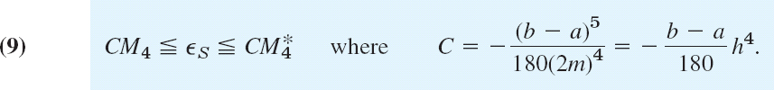
Degree of Precision (DP) of an integration formula. This is the maximum degree of arbitrary polynomials for which the formula gives exact values of integrals over any intervals.
Hence for the trapezoidal rule,
![]()
because we approximate the curve of f by portions of straight lines (linear polynomials).
For Simpson's rule we might expect DP = 2 (why?). Actually,
![]()
by (9) because f(4) is identically zero for a cubic polynomial. This makes Simpson's rule sufficiently accurate for most practical problems and accounts for its popularity.
Numeric Stability with respect to rounding is another important property of Simpson's rule. Indeed, for the sum of the roundoff errors ![]() j of the 2m + 1 values fj in (7) we obtain, since h = (b − a)/2m,
j of the 2m + 1 values fj in (7) we obtain, since h = (b − a)/2m,

where u is the rounding unit (![]() if we round off to 6D; see Sec. 19.1). Also 6 = 1 + 4 + 1 is the sum of the coefficients for a pair of intervals in (7); take m = 1 in (7) to see this. The bound (b − a)u is independent of m, so that it cannot increase with increasing m, that is, with decreasing h. This proves stability.
if we round off to 6D; see Sec. 19.1). Also 6 = 1 + 4 + 1 is the sum of the coefficients for a pair of intervals in (7); take m = 1 in (7) to see this. The bound (b − a)u is independent of m, so that it cannot increase with increasing m, that is, with decreasing h. This proves stability.
Newton–Cotes Formulas. We mention that the trapezoidal and Simpson rules are special closed Newton–Cotes formulas, that is, integration formulas in which f(x) is interpolated at equally spaced nodes by a polynomial of degree n(n = 1 for trapezoidal, n = 2 for Simpson), and closed means that a and b are nodes (a = x0, b = xn). n = 3 and higher n are used occasionally. From n = 8 on, some of the coefficients become negative, so that a positive fj could make a negative contribution to an integral, which is absurd. For more on this topic see Ref. [E25] in App. 1.
EXAMPLE 3 Simpson's Rule. Error Estimate
Evaluate ![]() by Simpson's rule with 2m = 10 and estimate the error.
by Simpson's rule with 2m = 10 and estimate the error.
Solution. Since h = 0.1, Table 19.5 gives
![]()
Estimate of error. Differentiation gives ![]() By considering the derivative f(5) of f(4) we find that the largest value of f(4) in the interval of integration occurs at 0 and the smallest value at
By considering the derivative f(5) of f(4) we find that the largest value of f(4) in the interval of integration occurs at 0 and the smallest value at ![]() . Computation gives the values M4 = f(4)(0) = 12 and
. Computation gives the values M4 = f(4)(0) = 12 and ![]() Since 2m = 10 and b − a = 1, we obtain C = −1/1800000 = −0.00000056. Therefore, from (9),
Since 2m = 10 and b − a = 1, we obtain C = −1/1800000 = −0.00000056. Therefore, from (9),
![]()
Hence J must lie between 0.746825 − 0.000007 = 0.746818 and 0.746825 + 0.000005 = 0.746830, so that at least four digits of our approximate value are exact. Actually, the value 0.746825 is exact to 5D because J = 0.746824 (exact to 6D).
Thus our result is much better than that in Example 1 obtained by the trapezoidal rule, whereas the number of operations is nearly the same in both cases.
Table 19.5 Computations in Example 3
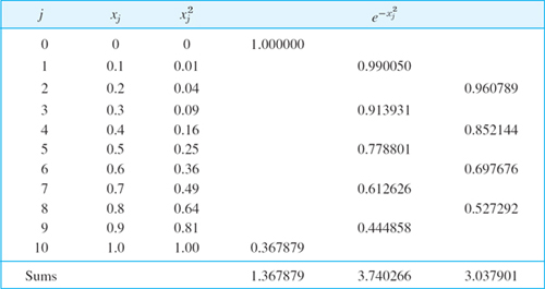
Instead of picking an n = 2m and then estimating the error by (9), as in Example 3, it is better to require an accuracy (e.g., 6D) and then determine n = 2m from (9).
EXAMPLE 4 Determination of n = 2m in Simpson's Rule from the Required Accuracy
What n should we choose in Example 3 to get 6D-accuracy?
Solution. Using M4 = 12 (which is bigger in absolute value than ![]() , we get from (9), with b − a = 1 and the required accuracy,
, we get from (9), with b − a = 1 and the required accuracy,
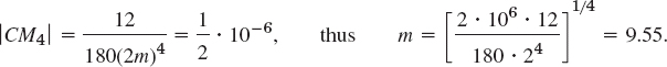
Hence we should choose n = 2m = 20. Do the computation, which parallels that in Example 3.
Note that the error bounds in (4) or (9) may sometimes be loose, so that in such a case a smaller n = 2m may already suffice.
Error Estimation for Simpson's Rule by Halving h. The idea is the same as in (5) and gives

Jh is obtained by using h and Jh/2 by using ![]() and
and ![]() h/2 is the error of Jh/2.
h/2 is the error of Jh/2.
Derivation. In (5) we had ![]() as the reciprocal of 3 = 4 − 1 and
as the reciprocal of 3 = 4 − 1 and ![]() resulted from h2 in (3) by replacing h with
resulted from h2 in (3) by replacing h with ![]() h. In (10) we have
h. In (10) we have ![]() as the reciprocal of 15 = 16 − 1 and
as the reciprocal of 15 = 16 − 1 and ![]() results from h4 in (8) by replacing h with
results from h4 in (8) by replacing h with ![]() h.
h.
EXAMPLE 5 Error Estimation for Simpson's Rule by Halving
Integrate ![]() from 0 to 2 with h = 1 and apply (10).
from 0 to 2 with h = 1 and apply (10).
Solution. The exact 5D-value of the integral is j = 1.25953. Simpson's rule gives

Hence (10) gives ![]() and thus J ≈ Jh/2 +
and thus J ≈ Jh/2 + ![]() h/2 = 1.26256 with an error −0.00283 which is less in absolute value than
h/2 = 1.26256 with an error −0.00283 which is less in absolute value than ![]() of the error 0.02979 of Jh/2. Hence the use of (10) was well worthwhile.
of the error 0.02979 of Jh/2. Hence the use of (10) was well worthwhile.
Adaptive Integration
The idea is to adapt step h to the variability of f(x). That is, where f varies but little, we can proceed in large steps without causing a substantial error in the integral, but where f varies rapidly, we have to take small steps in order to stay everywhere close enough to the curve of f.
Changing h is done systematically, usually by halving h, and automatically (not “by hand”) depending on the size of the (estimated) error over a subinterval. The subinterval is halved if the corresponding error is still too large, that is, larger than a given tolerance TOL (maximum admissible absolute error), or is not halved if the error is less than or equal to TOL (or doubled if the error is very small).
Adapting is one of the techniques typical of modern software. In connection with integration it can be applied to various methods. We explain it here for Simpson's rule. In Table 19.6 an asterisk means that for that subinterval, TOL has been reached.
EXAMPLE 6 Adaptive Integration with Simpson's Rule
Integrate ![]() from x = 0 to 2 by adaptive integration and with Simpson's rule and TOL[0, 2] = 0.0002.
from x = 0 to 2 by adaptive integration and with Simpson's rule and TOL[0, 2] = 0.0002.
Solution. Table 19.6 shows the calculations. Figure 444 shows the integrand f(x) and the adapted intervals used. The first two intervals ([0, 0.5], [0.5, 1.0]) have length 0.5, hence h = 0.25 [because we use 2m = 2 subintervals in Simpson's rule (7**)]. The next two intervals ([1.00, 1.25], [1.25, 1.50]) have length 0.25 (hence h = 0.125) and the last four intervals have length 0.125. Sample computations. For 0.740480 see Example 5. Formula (10) gives (0.123716 − 0.122794)/15 = 0.000061. Note that 0.123716 refers to [0, 0.5] and [0.5, 1], so that we must subtract the value corresponding to [0, 1] in the line before. Etc. TOL[0, 2] = 0.0002 gives 0.0001 for subintervals of length 1, 0.00005 for length 0.5, etc. The value of the integral obtained is the sum of the values marked by an asterisk (for which the error estimate has become less than TOL). This gives
![]()
The exact 5D-value is j = 1.25953. Hence the error is 0.00017. This is about 1/200 of the absolute value of that in Example 5. Our more extensive computation has produced a much better result.
Table 19.6 Computations in Example 6


Fig. 444. Adaptive integration in Example 6
Gauss Integration Formulas Maximum Degree of Precision
Our integration formulas discussed so far use function values at predetermined (equidistant) x-values (nodes) and give exact results for polynomials not exceeding a certain degree [called the degree of precision; see after (9)]. But we can get much more accurate integration formulas as follows. We set

with fixed n, and t = ±1 obtained from x = a, b by setting ![]() Then we determine the n coefficients A1, …, An and n nodes t1, …, tn so that (11) gives exact results for polynomials of degree k as high as possible. Since n + n = 2n is the number of coefficients of a polynomial of degree 2n − 1, it follows that k
Then we determine the n coefficients A1, …, An and n nodes t1, …, tn so that (11) gives exact results for polynomials of degree k as high as possible. Since n + n = 2n is the number of coefficients of a polynomial of degree 2n − 1, it follows that k ![]() 2n − 1.
2n − 1.
Gauss has shown that exactness for polynomials of degree not exceeding 2n − 1 (instead of n − 1 for predetermined nodes) can be attained, and he has given the location of the tj(= the jth zero of the Legendre polynomial Pn in Sec. 5.3) and the coefficients Aj which depend on n but not on f(t), and are obtained by using Lagrange's interpolation polynomial, as shown in Ref. [E5] listed in App. 1. With these tj and Aj formula (11) is called a Gauss integration formula or Gauss quadrature formula. Its degree of precision is 2n − 1 as just explained. Table 19.7 gives the values needed for n = 2, …, 5. (For larger n, see pp. 916−919 of Ref. [GenRef1] in App. 1.)
Table 19.7 Gauss Integration: Nodes tj and Coefficients Aj
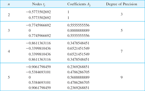
EXAMPLE 7 Gauss Integration Formula with n = 3
Evaluate the integral in Example 3 by the Gauss integration formula (11) with n = 3.
Solution. We have to convert our integral from 0 to 1 into an integral from −1 to 1. We set ![]() Then
Then ![]() and (11) with n = 3 and the above values of the nodes and the coefficients yields
and (11) with n = 3 and the above values of the nodes and the coefficients yields

(exact to 6D: 0.746825), which is almost as accurate as the Simpson result obtained in Example 3 with a much larger number of arithmetic operations. With 3 function values (as in this example) and Simpson's rule we would get ![]() with an error over 30 times that of the Gauss integration.
with an error over 30 times that of the Gauss integration.
EXAMPLE 8 Gauss Integration Formula with n = 4 and 5
Integrate ![]() from x = 0 to 2 by Gauss. Compare with the adaptive integration in Example 6 and comment.
from x = 0 to 2 by Gauss. Compare with the adaptive integration in Example 6 and comment.
Solution. x = t + 1 gives ![]() as needed in (11). For n = 4 we calculate (6S)
as needed in (11). For n = 4 we calculate (6S)

The error is 0.00003 because J = 1.25953 (6S). Calculating with 10S and n = 4 gives the same result; so the error is due to the formula, not rounding. For n = 5 and 10S we get J ≈ 1.259526185, too large by the amount 0.000000250 because J = 1.259525935 (10S). The accuracy is impressive, particularly if we compare the amount of work with that in Example 6.
Gauss integration is of considerable practical importance. Whenever the integrand f is given by a formula (not just by a table of numbers) or when experimental measurements can be set at times tj (or whatever t represents) shown in Table 19.7 or in Ref. [GenRef1], then the great accuracy of Gauss integration outweighs the disadvantage of the complicated tJ and Aj (which may have to be stored). Also, Gauss coefficients Aj are positive for all n, in contrast with some of the Newton–Cotes coefficients for larger n.
Of course, there are frequent applications with equally spaced nodes, so that Gauss integration does not apply (or has no great advantage if one first has to get the tj in (11) by interpolation).
Since the endpoints −1 and 1 of the interval of integration in (11) are not zeros of Pn, they do not occur among t0, …, tn, and the Gauss formula (11) is called, therefore, an open formula, in contrast with a closed formula, in which the endpoints of the interval of integration t0 are tn. and [For example, (2) and (7) are closed formulas.]
Numeric Differentiation
Numeric differentiation is the computation of values of the derivative of a function f from given values of f. Numeric differentiation should be avoided whenever possible. Whereas integration is a smoothing process and is not very sensitive to small inaccuracies in function values, differentiation tends to make matters rough and generally gives values of f′ that are much less accurate than those of f. The difficulty with differentiation is tied in with the definition of the derivative, which is the limit of the difference quotient, and, in that quotient, you usually have the difference of a large quantity divided by a small quantity. This can cause numerical instability. While being aware of this caveat, we must still develop basic differentiation formulas for use in numeric solutions of differential equations.
We use the notations ![]() etc., and may obtain rough approximation formulas for derivatives by remembering that
etc., and may obtain rough approximation formulas for derivatives by remembering that


Similarly, for the second derivative we obtain

More accurate approximations are obtained by differentiating suitable Lagrange polynomials. Differentiating (6) and remembering that the denominators in (6) are 2h2, −h2, 2h2, we have

Evaluating this at x0, x1, x2, we obtain the “three-point formulas”

Applying the same idea to the Lagrange polynomial p4(x), we obtain similar formulas, in particular,

Some examples and further formulas are included in the problem set as well as in Ref. [E5] listed in App. 1.
1–6 RECTANGULAR AND TRAPEZOIDAL RULES
- Rectangular rule. Evaluate the integral in Example 1 by the rectangular rule (1) with subintervals of length 0.1. Compare with Example 1. (6S-exact: 0.746824)
- Bounds for (1). Derive a formula for lower and upper bounds for the rectangular rule. Apply it to Prob. 1.
- Trapezoidal rule. To get a feel for increase in accuracy, integrate x2 from 0 to 1 by (2) with h = 1, 0.5, 0.25, 0.1.
- Error estimation by halfing. Integrate f(x) = x4 from 0 to 1 by (2) with h = 1, h = 0.5, h = 0.25 and estimate the error for h = 0.5 and h = 0.25 by (5).
- Error estimation. Do the tasks in Prob. 4 for

- Stability. Prove that the trapezoidal rule is stable with respect to rounding.
7–15 SIMPSON'S RULE
Evaluate the integrals ![]()
![]() by Simpson's rule with 2m as indicated, and compare with the exact value known from calculus.
by Simpson's rule with 2m as indicated, and compare with the exact value known from calculus.
- 7. A, 2m = 4
- 8. A, 2m = 10
- 9. B, 2m = 4
- 10. B, 2m = 10
- 11. J, 2m = 4
- 12. J, 2m = 10
- 13. Error estimate. Compute the integral J by Simpson's rule with 2m = 8 and use the value and that in Prob. 11 to estimate the error by (10).
- 14. Error bounds and estimate. Integrate e−x from 0 to 2 by (7) with h = 1 and with h = 0.5. Give error bounds for the h = 0.5 value and an error estimate by (10).
- 15. Given TOL. Find the smallest n in computing A (see Probs. 7 and 8) such that 5S-accuracy is guaranteed (a) by (4) in the use of (2), (b) by (9) in the use of (7).
16–21 NONELEMENTARY INTEGRALS
The following integrals cannot be evaluated by the usual methods of calculus. Evaluate them as indicated. Compare your value with that possibly given by your CAS. Si(x) is the sine integral. S(x) and C(x) are the Fresnel integrals. See App. A3.1. They occur in optics.

- 16. Si(1) by (2), n = 5, n = 10, and apply (5).
- 17. Si(1) by (7), 2m = 4
- 18. Obtain a better value in Prob. 17. Hint. Use (10).
- 19. Si(1) by (7), 2m = 10
- 20. S(1.25) by (7), 2m = 10
- 21. C(1.25) by (7), 2m = 10
22–25 GAUSS INTEGRATION
Integrate by (11) with n = 5:
- 22. cos x from 0 to
 π
π - 23. xe−x from 0 to 1
- 24. sin (x2) from 0 to 1.25
- 25. exp (−x2) from 0 to 1
- 26. TEAM PROJECT. Romberg Integration (W. Romberg, Norske Videnskab. Trondheim, Førh. 28, Nr. 7, 1955). This method uses the trapezoidal rule and gains precision stepwise by halving h and adding an error estimate. Do this for the integral of f(x) = e−x from x = 0 to x = 2 with TOL = 10−3, as follows.
Step 1. Apply the trapezoidal rule (2) with h = 2 (hence n = 1) to get an approximation J11. Halve h and use (2) to get J21 and an error estimate

If |
 21| TOL, stop. The result is J22 = J21 + 21.
Step 2. Show that
21 = −0.066596, hence |21| > TOL and go on. Use (2) with h/4 to get J31 and add to it the error estimate  to get the better J32 = J31 + 31. Calculate
If |
32| TOL, stop. The result is J33 = J32 + 32. (Why does 24 = 16 come in?) Show that we obtain 32 = −0.000266, so that we can stop. Arrange your J- and -values in a kind of “difference table.”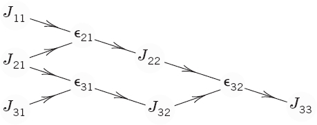
If |
32| were greater than TOL, you would have to go on and calculate in the next step J41 from (2) with  then
then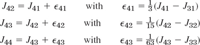
where 63 = 26 − 1. (How does this come in?)
Apply the Romberg method to the integral of
 from x = 0 to 2 with TOL = 10−4.
27–30 DIFFERENTIATION
- 27. Consider f(x) = x4 for x0 = 0, x1 = 0.2, x2 = 0.4, x3 = 0.6, x4 = 0.8. Calculate
 from (14a), (14b), (14c), (15). Determine the errors. Compare and comment.
 - 28. A “four-point formula” for the derivative is
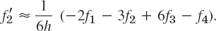
Apply it to f(x) = x4 with x1, …, x4 as in Prob. 27, determine the error, and compare it with that in the case of (15).
- 29. The derivative f′(x) can also be approximated in terms of first-order and higher order differences (see Sec. 19.3):

Compute f′(0.4) in Prob. 27 from this formula, using differences up to and including first order, second order, third order, fourth order.
- 30. Derive the formula in Prob. 29 from (14) in Sec. 19.3.
CHAPTER 19 REVIEW QUESTIONS AND PROBLEMS
- What is a numeric method? How has the computer influenced numerics?
- What is an error? A relative error? An error bound?
- Why are roundoff errors important? State the rounding rules.
- What is an algorithm? Which of its properties are important in software implementation?
- What do you know about stability?
- Why is the selection of a good method at least as important on a large computer as it is on a small one?
- Can the Newton (–Raphson) method diverge? Is it fast? Same questions for the bisection method.
- What is fixed-point iteration?
- What is the advantage of Newton's interpolation formulas over Lagrange's?
- What is spline interpolation? Its advantage over polynomial interpolation?
- List and compare the integration methods we have discussed.
- How did we use an interpolation polynomial in deriving Simpson's rule?
- What is adaptive integration? Why is it useful?
- In what sense is Gauss integration optimal?
- How did we obtain formulas for numeric differentiation?
- Write −46.9028104, 0.000317399, 54/7, −890/3 in floating-point form with 5S (5 significant digits, properly rounded).
- Compute (5.346 − 3.644)/(3.444 − 3.055) as given and then rounded stepwise to 3S, 2S, 1S. Comment. (“Stepwise” means rounding the rounded numbers, not the given ones.)
- Compute 0.38755/(5.6815 − 0.38419) as given and then rounded stepwise to 4S, 3S, 2S, 1S. Comment.
- Let 19.1 and 25.84 be correctly rounded. Find the shortest interval in which the sum s of the true (unrounded) numbers must lie.
- Do the same task as in Prob. 19 for the difference 3.2 − 6.29.
- What is the relative error of n
 in terms of that of ?
 - Show that the relative error of
 is about twice that of .
 - Solve x2 − 40x + 2 = 0 in two ways (cf. Sec. 19.1). Use 4S-arithmetic.
- Solve x2 − 100x + 1 = 0. Use 5S-arithmetic.
- Compute the solution of x4 = x + 0.1 near x = 0 by transforming the equation algebraically to the form x = g(x) and starting from x0 = 0.
- Solve cos x = x2 by Newton's method, starting from x = 0.5.
- Solve Prob. 25 by bisection (3S-accuracy).
- Compute sinh 0.4 from sinh 0, sinh 0.5 = 0.521, sinh 1.0 = 1.175 by quadratic interpolation.
- Find the cubic spline for the data f(0) = 0, f(1) = 0, f(2) = 4, k0 = −1, k2 = 5.
- Find the cubic spline q and the interpolation polynomial p for the data (0, 0), (1, 1), (2, 6), (3, 10), with q′(0) = 0, q′(3) = 0 and graph p and q on common axes.
- Compute the integral of x3 from 0 to 1 by the trapezoidal rule with n = 5. What error bounds are obtained from (4) in Sec. 19.5? What is the actual error of the result?
- Compute the integral of cos(x2) from 0 to 1 by Simpson's rule with 2m = 4.
- Solve Prob. 32 by Gauss integration with n = 3 and n = 5.
- Compute f′(0.2) for f(x) = x3 using (14b) in Sec. 19.5 with (a) h = 0.2, (b) h = 0.1. Compare the accuracy.
- Compute f″(0.2) for f(x) = x2 using (13) in Sec. 19.5 with (a) h = 0.2, (b) h = 0.1.
SUMMARY OF CHAPTER 19 Numerics in General
In this chapter we discussed concepts that are relevant throughout numeric work as a whole and methods of a general nature, as opposed to methods for linear algebra (Chap. 20) or differential equations (Chap. 21).
In scientific computations we use the floating-point representation of numbers (Sec. 19.1); fixed-point representation is less suitable in most cases.
Numeric methods give approximate values ![]() of quantities. The error
of quantities. The error ![]() of
of ![]() is
is
![]()
where a is the exact value. The relative error of ![]() is
is ![]() /a. Errors arise from rounding, inaccuracy of measured values, truncation (that is, replacement of integrals by sums, series by partial sums), and so on.
/a. Errors arise from rounding, inaccuracy of measured values, truncation (that is, replacement of integrals by sums, series by partial sums), and so on.
An algorithm is called numerically stable if small changes in the initial data give only correspondingly small changes in the final results. Unstable algorithms are generally useless because errors may become so large that results will be very inaccurate. The numeric instability of algorithms must not be confused with the mathematical instability of problems (“ill-conditioned problems,” Sec. 19.2).
Fixed-point iteration is a method for solving equations f(x) = 0 in which the equation is first transformed algebraically to x = g(x), an initial guess x0 for the solution is made, and then approximations x1, x2, …, are successively computed by iteration from (see Sec. 19.2)
![]()
Newton's method for solving equations f(x) = 0 is an iteration

Here xn+1 is the x-intercept of the tangent of the curve y = f(x) at the point xn. This method is of second order (Theorem 2, Sec. 19.2). If we replace f′ in (3) by a difference quotient (geometrically: we replace the tangent by a secant), we obtain the secant method; see (10) in Sec. 19.2. For the bisection method (which converges slowly) and the method of false position, see Problem Set 19.2.
Polynomial interpolation means the determination of a polynomial pn(x) such that pn(xj) = fj, where j = 0, …, n and (x0, f0), …, (xn, fn) are measured or observed values, values of a function, etc. pn(x) is called an interpolation polynomial. For given data, pn(x) of degree n (or less) is unique. However, it can be written in different forms, notably in Lagrange's form (4), Sec. 19.3, or in Newton's divided difference form (10), Sec. 19.3, which requires fewer operations. For regularly spaced x0, x1 = x0 + h, …, xn = x0 + nh the latter becomes Newton's forward difference formula (formula (14) in Sec. 19.3):

where r = (x − x0)/h and the forward differences are Δfj = fj+1 − fj and
![]()
A similar formula is Newton's backward difference interpolation formula (formula (18) in Sec. 19.3).
Interpolation polynomials may become numerically unstable as n increases, and instead of interpolating and approximating by a single high-degree polynomial it is preferable to use a cubic spline g(x), that is, a twice continuously differentiable interpolation function [thus, g(xj) = fj], which in each subinterval xj ![]() x
x ![]() xj+1 consists of a cubic polynomial qj(x); see Sec. 19.4.
xj+1 consists of a cubic polynomial qj(x); see Sec. 19.4.
Simpson's rule of numeric integration is [see (7), Sec. 19.5]

with equally spaced nodes xj = x0 + jh, j = 1, …, 2m, h = (b − a)/(2m), and fj = f(xj). It is simple but accurate enough for many applications. Its degree of precision is DP = 3 because the error (8), Sec. 19.5, involves h4. A more practical error estimate is (10), Sec. 19.5,
![]()
obtained by first computing with step h, then with step h/2, and then taking ![]() of the difference of the results.
of the difference of the results.
Simpson's rule is the most important of the Newton–Cotes formulas, which are obtained by integrating Lagrange interpolation polynomials, linear ones for the trapezoidal rule (2), Sec. 19.5, quadratic for Simpson's rule, cubic for the three-eights rule (see the Chap. 19 Review Problems), etc.
Adaptive integration (Sec. 19.5, Example 6) is integration that adjusts (“adapts”) the step (automatically) to the variability of f(x).
Romberg integration (Team Project 26, Problem Set 19.5) starts from the trapezoidal rule (2), Sec. 19.5, with h, h/2, h/4, etc. and improves results by systematically adding error estimates.
Gauss integration (11), Sec. 19.5, is important because of its great accuracy (DP = 2n − 1, compared to Newton–Cotes's DP = n − 1 or n). This is achieved by an optimal choice of the nodes, which are not equally spaced; see Table 19.7, Sec. 19.5.
Numeric differentiation is discussed at the end of Sec. 19.5. (Its main application (to differential equations) follows in Chap. 21.)
1JOSEPH RAPHSON (1648–1715), English mathematician who published a method similar to Newton's method. For historical details, see Ref. [GenRef2], p. 203, listed in App. 1.
2JAMES GREGORY (1638–1675), Scots mathematician, professor at St. Andrews and Edinburgh. Δ in (14) and ∇2 (on p. 818) have nothing to do with the Laplacian.
3CARL RUNGE (1856–1927), German mathematician, also known for his work on ODEs (Sec. 21.1).
4THOMAS SIMPSON (1710–1761), self-taught English mathematician, author of several popular textbooks. Simpson's rule was used much earlier by Torricelli, Gregory (in 1668), and Newton (in 1676).