
CHAPTER 15
Power Series, Taylor Series

In Chapter 14, we evaluated complex integrals directly by using Cauchy's integral formula, which was derived from the famous Cauchy integral theorem. We now shift from the approach of Cauchy and Goursat to another approach of evaluating complex integrals, that is, evaluating them by residue integration. This approach, discussed in Chapter 16, first requires a thorough understanding of power series and, in particular, Taylor series. (To develop the theory of residue integration, we still use Cauchy's integral theorem!)
In this chapter, we focus on complex power series and in particular Taylor series. They are analogs of real power series and Taylor series in calculus. Section 15.1 discusses convergence tests for complex series, which are quite similar to those for real series. Thus, if you are familiar with convergence tests from calculus, you may use Sec. 15.1 as a reference section. The main results of this chapter are that complex power series represent analytic functions, as shown in Sec. 15.3, and that, conversely, every analytic function can be represented by power series, called a Taylor series, as shown in Sec. 15.4. The last section (15.5) on uniform convergence is optional.
Sections that may be omitted in a shorter course: 15.1, 15.5.
References and Answers to Problems: App. 1 Part D, App. 2.
15.1 Sequences, Series, Convergence Tests
The basic concepts for complex sequences and series and tests for convergence and divergence are very similar to those concepts in (real) calculus. Thus if you feel at home with real sequences and series and want to take for granted that the ratio test also holds in complex, skip this section and go to Section 15.2.
Sequences
The basic definitions are as in calculus. An infinite sequence or, briefly, a sequence, is obtained by assigning to each positive integer n a number zn, called a term of the sequence, and is written
![]()
We may also write z0, z1, … or z2, z3, … or start with some other integer if convenient.
A real sequence is one whose terms are real.
Convergence. A convergent sequence z1, z2, … is one that has a limit c, written
![]()
By definition of limit this means that for every ![]() > 0 we can find an N such that
> 0 we can find an N such that
![]()
geometrically, all terms zn with n > N lie in the open disk of radius ![]() and center c (Fig. 361) and only finitely many terms do not lie in that disk. [For a real sequence, (1) gives an open interval of length 2
and center c (Fig. 361) and only finitely many terms do not lie in that disk. [For a real sequence, (1) gives an open interval of length 2![]() and real midpoint c on the real line as shown in Fig. 362.]
and real midpoint c on the real line as shown in Fig. 362.]
A divergent sequence is one that does not converge.

Fig. 361. Convergent complex sequence
![]()
Fig. 362. Convergent real sequence
EXAMPLE 1 Convergent and Divergent Sequences
The sequence ![]() is convergent with limit 0.
is convergent with limit 0.
The sequence {in} = {i, −1, −i, 1, …} is divergent, and so is {zn} with zn = (1 + i)n.
EXAMPLE 2 Sequences of the Real and the Imaginary Parts
The sequence {zn} with zn = xn + iyn = 1 − 1/n2 + i(2 + 4/n) is ![]() (Sketch it.) It converges with the limit c = 1 + 2i. Observe that {xn} has the limit 1 = Re c and {yn} has the limit 2 = Im c. This is typical. It illustrates the following theorem by which the convergence of a complex sequence can be referred back to that of the two real sequences of the real parts and the imaginary parts.
(Sketch it.) It converges with the limit c = 1 + 2i. Observe that {xn} has the limit 1 = Re c and {yn} has the limit 2 = Im c. This is typical. It illustrates the following theorem by which the convergence of a complex sequence can be referred back to that of the two real sequences of the real parts and the imaginary parts.
THEOREM 1 Sequences of the Real and the Imaginary Parts
A sequence z1, z2, …, zn, … of complex numbers zn = xn + yn (where n = 1, 2, …) converges to c = a + ib if and only if the sequence of the real parts x1, x2, … converges to a and the sequence of the imaginary parts y1, y2, … converges to b.
PROOF
Convergence zn → c = a + ib implies convergence xn → a and yn → b because if |zn − c| < ![]() then zn lies within the circle of radius
then zn lies within the circle of radius ![]() about c = a + ib so that (Fig. 363a)
about c = a + ib so that (Fig. 363a)
![]()
Conversely, if xn → a and yn → b as n → ∞, then for a given ![]() > 0 we can choose N so large that, for every n > N,
> 0 we can choose N so large that, for every n > N,
![]()
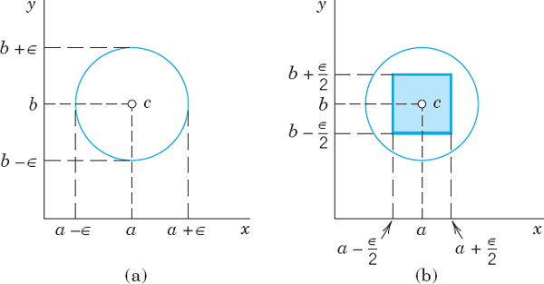
Fig. 363. Proof of Theorem 1
These two inequalities imply that zn = xn + iyn lies in a square with center c and side ![]() . Hence, zn must lie within a circle of radius
. Hence, zn must lie within a circle of radius ![]() with center c (Fig. 363b).
with center c (Fig. 363b).
Series
Given a sequence z1, z2, …, zm, …, we may form the sequence of the sums
![]()
and in general
![]()
Here sn is called the nth partial sum of the infinite series or series
The z1, z2, … are called the terms of the series. (Our usual summation letter is n, unless we need n for another purpose, as here, and we then use m as the summation letter.)
A convergent series is one whose sequence of partial sums converges, say,

and call s the sum or value of the series. A series that is not convergent is called a divergent series.
If we omit the terms of sn from (3), there remains
![]()
This is called the remainderof the series (3) after the term zn. Clearly, if (3) converges and has the sum s, then
![]()
Now sn → s by the definition of convergence; hence Rn → 0. In applications, when s is unknown and we compute an approximation sn of s, then |Rn| is the error, and Rn → 0 means that we can make |Rn| as small as we please, by choosing n large enough.
An application of Theorem 1 to the partial sums immediately relates the convergence of a complex series to that of the two series of its real parts and of its imaginary parts:
THEOREM 2 Real and Imaginary Parts
A series (3) with zm = xm + iym converges and has the sum s = u + iv if and only if x1 + x2 + … converges and has the sum u and y1 + y2 + … converges and has the sum v.
Tests for Convergence and Divergence of Series
Convergence tests in complex are practically the same as in calculus. We apply them before we use a series, to make sure that the series converges.
Divergence can often be shown very simply as follows.
If a series z1 + z2 + … converges, then ![]() Hence if this does not hold, the series diverges.
Hence if this does not hold, the series diverges.
PROOF
If z1 + z2 + … converges, with the sum s, then, since zm = sm − sm−1,
![]()
CAUTION! zm → 0 is necessary for convergence but not sufficient, as we see from the harmonic series ![]() which satisfies this condition but diverges, as is shown in calculus (see, for example, Ref. [GenRef11] in App. 1).
which satisfies this condition but diverges, as is shown in calculus (see, for example, Ref. [GenRef11] in App. 1).
The practical difficulty in proving convergence is that, in most cases, the sum of a series is unknown. Cauchy overcame this by showing that a series converges if and only if its partial sums eventually get close to each other:
THEOREM 4 Cauchy's Convergence Principle for Series
A series z1 + z2 + … is convergent if and only if for every given ![]() > 0 (no matter how small) we can find an N (which depends on
> 0 (no matter how small) we can find an N (which depends on ![]() , in general) such that
, in general) such that
![]()
The somewhat involved proof is left optional (see App. 4).
Absolute Convergence. A series z1 + z2 + … is called absolutely convergent if the series of the absolute values of the terms

is convergent.
If z1 + z2 + … converges but |z1| + |z2| + … diverges, then the series z1 + z2 + … is called, more precisely, conditionally convergent.
EXAMPLE 3 A Conditionally Convergent Series
The series ![]() converges, but only conditionally since the harmonic series diverges, as mentioned above (after Theorem 3).
converges, but only conditionally since the harmonic series diverges, as mentioned above (after Theorem 3).
If a series is absolutely convergent, it is convergent.
This follows readily from Cauchy's principle (see Prob. 29). This principle also yields the following general convergence test.
If a series z1 + z2 + … is given and we can find a convergent series b1 + b2 + … with nonnegative real terms such that |z1| ![]() b1, |z2|
b1, |z2| ![]() b2, …, then the given series converges, even absolutely.
b2, …, then the given series converges, even absolutely.
PROOF
By Cauchy's principle, since b1 + b2 + … converges, for any given ![]() > 0 we can find an N such that
> 0 we can find an N such that
![]()
From this and |z1| ![]() b1, |z2|
b1, |z2| ![]() b2, … we conclude that for those n and p,
b2, … we conclude that for those n and p,
![]()
Hence, again by Cauchy's principle, |z1| + |z2| + … converges, so that z1 + z2 + … is absolutely convergent.
A good comparison series is the geometric series, which behaves as follows.
The geometric series

converges with the sum 1/(1 − q) if |q| < 1 and diverges if |q| ![]() 1.
1.
PROOF
If |q| ![]() 1, then |qm|
1, then |qm| ![]() 1 and Theorem 3 implies divergence.
1 and Theorem 3 implies divergence.
Now let |q| < 1. The nth partial sum is
![]()
From this,
![]()
On subtraction, most terms on the right cancel in pairs, and we are left with
![]()
Now 1 − q ≠ 0 since q ≠ 1, and we may solve for sn finding
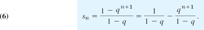
Since |q| < 1, the last term approaches zero as n → ∞. Hence if |q| < 1. the series is convergent and has the sum 1/(1 − q). This completes the proof.
Ratio Test
This is the most important test in our further work. We get it by taking the geometric series as comparison series b1 + b2 + … in Theorem 5:
If a series z1 + z2 + … with zn ≠ 0 (n = 1, 2, …) has the property that for every n greater than some N,

(where q < 1 is fixed), this series converges absolutely. If for every n > N,

the series diverges.
PROOF
If (8) holds, then |zn + 1| ![]() |zn| for n > N, so that divergence of the series follows from Theorem 3.
|zn| for n > N, so that divergence of the series follows from Theorem 3.
If (7) holds, then |zn + 1| ![]() |zn| q for n > N, in particular,
|zn| q for n > N, in particular,
![]()
and in general, |zN + p| ![]() |zN + 1|qp−1. Since q < 1, we obtain from this and Theorem 6
|zN + 1|qp−1. Since q < 1, we obtain from this and Theorem 6
![]()
Absolute convergence of z1 + z2 + … now follows from Theorem 5.
CAUTION! The inequality (7) implies |zn + 1/zn| < 1, but this does not imply convergence, as we see from the harmonic series, which satisfies zn + 1/zn = n/(n + 1) < 1 for all n but diverges.
If the sequence of the ratios in (7) and (8) converges, we get the more convenient
If a series z1 + z2 + … with zn ≠ 0(n = 1, 2, …) is such that ![]() then:
then:
- If L < 1, the series converges absolutely.
- If L > 1, the series diverges.
- If L = 1, the series may converge or diverge, so that the test fails and permits no conclusion.
PROOF
(a) We write kn = |zn + 1/zn| and let L = 1 − b < 1. Then by the definition of limit, the kn must eventually get close to 1 − b, say, ![]() for all n greater than some N. Convergence of z1 + z2 + … now follows from Theorem 7.
for all n greater than some N. Convergence of z1 + z2 + … now follows from Theorem 7.
(b) Similarly, for L = 1 + c > 1 we have ![]() for all n > N* (sufficiently large), which implies divergence of z1 + z2 + … by Theorem 7.
for all n > N* (sufficiently large), which implies divergence of z1 + z2 + … by Theorem 7.
(c) The harmonic series ![]() has zn + 1/zn = n/(n + 1), hence L = 1, and diverges. The series
has zn + 1/zn = n/(n + 1), hence L = 1, and diverges. The series

hence also L = 1, but it converges. Convergence follows from (Fig. 364)

so that s1, s2, … is a bounded sequence and is monotone increasing (since the terms of the series are all positive); both properties together are sufficient for the convergence of the real sequence s1, s2, …. (In calculus this is proved by the so-called integral test, whose idea we have used.)

Fig. 364. Convergence of the series 1 +14 +19 +116 + …
Is the following series convergent or divergent? (First guess, then calculate.)

Solution. By Theorem 8, the series is convergent, since
![]()
EXAMPLE 5 Theorem 7 More General Than Theorem 8
Let an = i/23n and bn = 1/23n + 1. Is the following series convergent or divergent?

Solution. The ratios of the absolute values of successive terms are ![]() Hence convergence follows from Theorem 7. Since the sequence of these ratios has no limit, Theorem 8 is not applicable.
Hence convergence follows from Theorem 7. Since the sequence of these ratios has no limit, Theorem 8 is not applicable.
Root Test
The ratio test and the root test are the two practically most important tests. The ratio test is usually simpler, but the root test is somewhat more general.
If a series z1 + z2 + … is such that for every n greater than some N,
![]()
(where q < 1 is fixed), this series converges absolutely. If for infinitely many n,
![]()
the series diverges.
PROOF
If (9) holds, then |zn| ![]() qn < 1 for all n > N. Hence the series |z1| + |z2| + … converges by comparison with the geometric series, so that the series z1 + z2 + … converges absolutely. If (10) holds, then |zn|
qn < 1 for all n > N. Hence the series |z1| + |z2| + … converges by comparison with the geometric series, so that the series z1 + z2 + … converges absolutely. If (10) holds, then |zn| ![]() 1 for infinitely many n. Divergence of z1 + z2 + … now follows from Theorem 3.
1 for infinitely many n. Divergence of z1 + z2 + … now follows from Theorem 3.
CAUTION! Equation (9) implies ![]() but this does not imply convergence, as we see from the harmonic series, which satisfies
but this does not imply convergence, as we see from the harmonic series, which satisfies ![]() (for n > 1) but diverges.
(for n > 1) but diverges.
If the sequence of the roots in (9) and (10) converges, we more conveniently have
If a series z1 + z2 + … is such that ![]() then:
then:
- The series converges absolutely if L < 1.
- The series diverges if L > 1.
- If L = 1, the test fails; that is, no conclusion is possible.
1–10 SEQUENCES
Is the given sequence z1, z2, …, zn, … bounded? Convergent? Find its limit points. Show your work in detail.
- zn = (1 + i)2n/2n
- zn = (3 + 4i)n/n!
- zn = nπ/(4 + 2ni)
- zn = (1 + 2i)n
- zn = (−1)n + 10i
- zn = (cos nπi)/n
- zn = n2 + i/n2

- zn = (3 + 3i)−n

- CAS EXPERIMENT. Sequences. Write a program for graphing complex sequences. Use the program to discover sequences that have interesting “geometric” properties, e.g., lying on an ellipse, spiraling to its limit, having infinitely many limit points, etc.
- Addition of sequences. If z1, z2, … converges with the limit l and
 converges with the limit l*, show that
  is convergent with the limit l + l*.
 - Bounded sequence. Show that a complex sequence is bounded if and only if the two corresponding sequences of the real parts and of the imaginary parts are bounded.
- On Theorem 1. Illustrate Theorem 1 by an example of your own.
- On Theorem 2. Give another example illustrating Theorem 2.
16–25 SERIES
Is the given series convergent or divergent? Give a reason. Show details.
- 16.

- 17.

- 18.

- 19.

- 20.

- 21.

- 22.

- 23.

- 24.

- 25.

- 26. Significance of (7). What is the difference between (7) and just stating |zn + 1/zn| < 1?
- 27. On Theorems 7 and 8. Give another example showing that Theorem 7 is more general than Theorem 8.
- 28. CAS EXPERIMENT. Series. Write a program for computing and graphing numeric values of the first n partial sums of a series of complex numbers. Use the program to experiment with the rapidity of convergence of series of your choice.
- 29. Absolute convergence. Show that if a series converges absolutely, it is convergent.
- 30. Estimate of remainder. Let |zn + 1/zn|
 q < 1, so that the series z1 + z2 + … converges by the ratio test. Show that the remainder Rn = zn + 1 + zn + 2 + … satisfies the inequality |Rn| |zn + 1|/(1 − q). Using this, find how many terms suffice for computing the sum s of the series

with an error not exceeding 0.05 and compute s to this accuracy.
15.2 Power Series
The student should pay close attention to the material because we shall show how power series play an important role in complex analysis. Indeed, they are the most important series in complex analysis because their sums are analytic functions (Theorem 5, Sec. 15.3), and every analytic function can be represented by power series (Theorem 1, Sec. 15.4).
A power series in powers of z − z0 is a series of the form
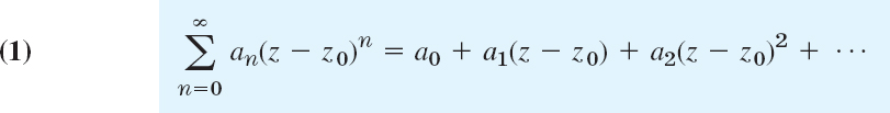
where z is a complex variable, a0, a1, … are complex (or real) constants, called the coefficients of the series, and z0 is a complex (or real) constant, called the center of the series. This generalizes real power series of calculus.
If z0 = 0, we obtain as a particular case a power series in powers of z:

Convergence Behavior of Power Series
Power series have variable terms (functions of z), but if we fix z, then all the concepts for series with constant terms in the last section apply. Usually a series with variable terms will converge for some z and diverge for others. For a power series the situation is simple. The series (1) may converge in a disk with center z0 or in the whole z-plane or only at z0. We illustrate this with typical examples and then prove it.
EXAMPLE 1 Convergence in a Disk. Geometric Series
The geometric series

converges absolutely if |z| < 1 and diverges if |z| ![]() 1 (see Theorem 6 in Sec. 15.1).
1 (see Theorem 6 in Sec. 15.1).
EXAMPLE 2 Convergence for Every z
The power series (which will be the Maclaurin series of ez in Sec. 15.4)

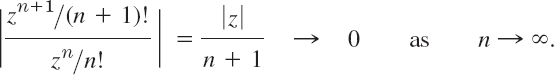
is absolutely convergent for every z. In fact, by the ratio test, for any fixed z,
EXAMPLE 3 Convergence Only at the Center. (Useless Series)
The following power series converges only at z = 0, but diverges for every z ≠ 0, as we shall show.

In fact, from the ratio test we have
![]()
THEOREM 1 Convergence of a Power Series
(a) Every power series (1) converges at the center z0
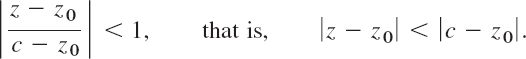
(b) If (1) converges at a point z = z1 ≠ z0, it converges absolutely for every z closer to z0 than z1, that is, |z − z0| < |z1 − z0|. See Fig. 365.
(c) If (1) diverges at z = z2, it diverges for every z farther away from z0 than z2. See Fig. 365.

PROOF
(a) For z = z0 the series reduces to the single term a0.
(b) Convergence at z = z1 gives by Theorem 3 in Sec. 15.1 an(z1 − z0)n → 0 as n → ∞. This implies boundedness in absolute value,
![]()
Multiplying and dividing an(z − z0)n by (z1 − z0)n we obtain from this

Summation over n gives

Now our assumption |z − z0| < |z1 − z0| implies that |(z − z0)/(z1 − z0)| < 1. Hence the series on the right side of (3) is a converging geometric series (see Theorem 6 in Sec. 15.1). Absolute convergence of (1) as stated in (b) now follows by the comparison test in Sec. 15.1.
(c) If this were false, we would have convergence at a z3 farther away from z0 than z2. This would imply convergence at z2, by (b), a contradiction to our assumption of divergence at z2.
Radius of Convergence of a Power Series
Convergence for every z (the nicest case, Example 2) or for no z ≠ z0 (the useless case, Example 3) needs no further discussion, and we put these cases aside for a moment. We consider the smallest circle with center z0 that includes all the points at which a given power series (1) converges. Let R denote its radius. The circle

is called the circle of convergence and its radius R the radius of convergence of (1). Theorem 1 then implies convergence everywhere within that circle, that is, for all z for which
![]()
(the open disk with center z0 and radius R). Also, since R is as small as possible, the series (1) diverges for all z for which
![]()
No general statements can be made about the convergence of a power series (1) on the circle of convergence itself. The series (1) may converge at some or all or none of the points. Details will not be important to us. Hence a simple example may just give us the idea.

Fig. 366. Circle of convergence
EXAMPLE 4 Behavior on the Circle of Convergence
On the circle of convergence (radius R = 1 in all three series),
Σ zn/n2 converges everywhere since Σ 1/n2 converges,
Σ zn/n converges at −1 (by Leibniz's test) but diverges at 1,
Σ zn diverges everywhere.
Notations R = ∞ and R = 0. To incorporate these two excluded cases in the present notation, we write
R = ∞ if the series (1) converges for all z (as in Example 2),
R = 0 if (1) converges only at the center z = z0 (as in Example 3).
These are convenient notations, but nothing else.
Real Power Series. In this case in which powers, coefficients, and center are real, formula (4) gives the convergence interval |x − x0| < R of length 2R on the real line.
Determination of the Radius of Convergence from the Coefficients. For this important practical task we can use
THEOREM 2 Radius of Convergence R
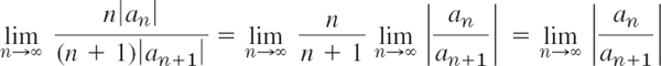
Suppose that the sequence |an + 1/an|, n = 1, 2, …, converges with limit L*. If L* = 0, then R = ∞; that is, the power series (1) converges for all z. If L* ≠ 0 (hence L* > 0), then

If |an + 1/an| → ∞, then R = 0 (convergence only at the center z0).
PROOF
For (1) the ratio of the terms in the ratio test (Sec. 15.1) is

Let L* ≠ 0, thus L* > 0. We have convergence if L = L*|z − z0| < 1, thus |z − z0| < 1/L*, and divergence if |z − z0| > 1/L*. By (4) and (5) this shows that 1/L* is the convergence radius and proves (6).
If L* = 0, then L = 0 for every z, which gives convergence for all z by the ratio test. If |an + 1/an| → ∞, then |an + 1/an||z − z0| > 1 for any z ≠ z0 and all sufficiently large n. This implies divergence for all z ≠ z0 by the ratio test (Theorem 7, Sec. 15.1).
Formula (6) will not help if L* does not exist, but extensions of Theorem 2 are still possible, as we discuss in Example 6 below.
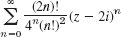
EXAMPLE 5 Radius of Convergence
By (6) the radius of convergence of the power series ![]() is
is
![]()
The series converges in the open disk ![]() of radius
of radius ![]() and center 3i.
and center 3i.
EXAMPLE 6 Extension of Theorem 2
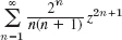
Find the radius of convergence R of the power series
![]()
Solution. The sequence of the ratios ![]() does not converge, so that Theorem 2 is of no help. It can be shown that
does not converge, so that Theorem 2 is of no help. It can be shown that
![]()
This still does not help here, since ![]() does not converge because
does not converge because ![]() for odd n, whereas for even n we have
for odd n, whereas for even n we have
![]()
so that ![]() has the two limit points
has the two limit points ![]() and 1. It can further be shown that
and 1. It can further be shown that
![]()
Here ![]() = I, so that R = 1. Answer. The series converges for |z| < 1.
= I, so that R = 1. Answer. The series converges for |z| < 1.
Summary. Power series converge in an open circular disk or some even for every z (or some only at the center, but they are useless); for the radius of convergence, see (6) or Example 6.
Except for the useless ones, power series have sums that are analytic functions (as we show in the next section); this accounts for their importance in complex analysis.
- Power series. Are 1/z + z + z2 + … and z + z3/2 + z2 + z3 + … power series? Explain.
- Radius of convergence. What is it? Its role? What motivates its name? How can you find it?
- Convergence. What are the only basically different possibilities for the convergence of a power series?
- On Examples 1–3. Extend them to power series in powers of z − 4 + 3πi. Extend Example 1 to the case of radius of convergence 6.
- Powers z2n. Show that if Σanzn has radius of convergence R (assumed finite), then Σanz2n has radius of convergence

6–18 RADIUS OF CONVERGENCE
Find the center and the radius of convergence.
- 6.

- 7.

- 8.

- 9.

- 10.

- 11.

- 12.

- 13.

- 14.

- 15.
- 16.

- 17.
- 18.

- 19. CAS PROJECT. Radius of Convergence. Write a program for computing R from (6), (6*), or (6**), in this order, depending on the existence of the limits needed. Test the program on some series of your choice such that all three formulas (6), (6*), and (6**) will come up.
- 20. TEAM PROJECT. Radius of Convergence. (a) Understanding (6). Formula (6) for R contains |an/an + 1|, not |an + 1/an|. How could you memorize this by using a qualitative argument?
(b) Change of coefficients. What happens to R (0 < R < ∞) if you (i) multiply all an by, k ≠ 0, (ii) multiply all an by Kn ≠ 0, (iii) replace an by 1/an? Can you think of an application of this?
(c) Understanding Example 6, which extends Theorem 2 to nonconvergent cases of an/an + 1. Do you understand the principle of “mixing” by which Example 6 was obtained? Make up further examples.
(d) Understanding (b) and (c) in Theorem 1. Does there exist a power series in powers of z that converges at z = 30 + 10i and diverges at z = 31 − 6i? Give reason.
15.3 Functions Given by Power Series
Here, our main goal is to show that power series represent analytic functions. This fact (Theorem 5) and the fact that power series behave nicely under addition, multiplication, differentiation, and integration accounts for their usefulness.
To simplify the formulas in this section, we take z0 = 0 and write

There is no loss of generality because a series in powers of ![]() − z0 with any z0 can always be reduced to the form (1) if we set
− z0 with any z0 can always be reduced to the form (1) if we set ![]() − z0 = z.
− z0 = z.
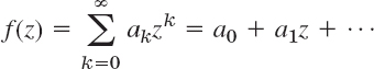
Terminology and Notation. If any given power series (1) has a nonzero radius of convergence R (thus R > 0), its sum is a function of z, say f(z). Then we write

We say that f(z) is represented by the power series or that it is developed in the power series. For instance, the geometric series represents the function f(z) = 1/(1 − z) in the interior of the unit circle |z| = 1. (See Theorem 6 in Sec. 15.1.)
Uniqueness of a Power Series Representation. This is our next goal. It means that a function f(z) cannot be represented by two different power series with the same center. We claim that if f(z) can at all be developed in a power series with center z0, the development is unique. This important fact is frequently used in complex analysis (as well as in calculus). We shall prove it in Theorem 2. The proof will follow from
THEROEM 1 Continuity of the Sum of a Power Series
If a function f(z) can be represented by a power series (2) with radius of convergence R > 0, then f(z) is continuous at z = 0.
From (2) with z = 0 we have f(0) = a0. Hence by the definition of continuity we must show that limz→0 f(z) = f(0) = a0. That is, we must show that for a given ![]() > 0 there is a δ > 0 such that |z| < δ implies |f(z) − a0| <
> 0 there is a δ > 0 such that |z| < δ implies |f(z) − a0| < ![]() . Now (2) converges absolutely for |z|
. Now (2) converges absolutely for |z| ![]() r with any r such that 0 < r < R, by Theorem 1 in Sec. 15.2. Hence the series
r with any r such that 0 < r < R, by Theorem 1 in Sec. 15.2. Hence the series

converges. Let S ≠ 0 be its sum. (S = 0 is trivial.) Then for 0 < |z| ![]() r,
r,

and |z|S < ![]() when |z| < δ, where δ > 0 is less than r and less than
when |z| < δ, where δ > 0 is less than r and less than ![]() /S. Hence |z|S < δS < (
/S. Hence |z|S < δS < (![]() /S)S =
/S)S = ![]() . This proves the theorem.
. This proves the theorem.
From this theorem we can now readily obtain the desired uniqueness theorem (again assuming z0 = 0 without loss of generality):
THEOREM 2 Identity Theorem for Power Series. Uniqueness
Let the power series a0 + a1z + a2z2 + … and b0 + b1z + b2z2 + … both be convergent for |z| < R, where R is positive, and let them both have the same sum for all these z. Then the series are identical, that is, a0 = b0, a1 = b1, a2 = b2, ….
Hence if a function f(z) can be represented by a power series with any center z0 this representation is unique.
PROOF
We proceed by induction. By assumption,
![]()
The sums of these two power series are continuous at z = 0, by Theorem 1. Hence if we consider |z| > 0 and let z → 0 on both sides, we see that a0 = b0: the assertion is true for n = 0. Now assume that an = bn for n = 0, 1, …, m. Then on both sides we may omit the terms that are equal and divide the result by zm + 1 (≠ 0); this gives
![]()
Similarly as before by letting z → 0 we conclude from this that am + 1 = bm + 1. This completes the proof.
Operations on Power Series
Interesting in itself, this discussion will serve as a preparation for our main goal, namely, to show that functions represented by power series are analytic.
Termwise addition or subtraction of two power series with radii of convergence R1 and R2 yields a power series with radius of convergence at least equal to the smaller of R1 and R2. Proof. Add (or subtract) the partial sums sn and ![]() term by term and use lim
term by term and use lim ![]()
Termwise multiplication of two power series
and

means the multiplication of each term of the first series by each term of the second series and the collection of like powers of z. This gives a power series, which is called the Cauchy product of the two series and is given by

We mention without proof that this power series converges absolutely for each z within the smaller circle of convergence of the two given series and has the sum s(z) = f(z)g(z). For a proof, see [D5] listed in App. 1.
Termwise differentiation and integration of power series is permissible, as we show next. We call derived series of the power series (1) the power series obtained from (1) by termwise differentiation, that is,

THEOREM 3 Termwise Differentiation of a Power Series
The derived series of a power series has the same radius of convergence as the original series.
PROOF
This follows from (6) in Sec. 15.2 because
or, if the limit does not exist, from (6**) in Sec. 15.2 by noting that ![]() as n → ∞.
as n → ∞.
EXAMPLE 1 Application of Theorem 3
Find the radius of convergence R of the following series by applying Theorem 3.

Solution. Differentiate the geometric series twice term by term and multiply the result by z2/2. This yields the given series. Hence R = 1 by Theorem 3.
THEOREM 4 Termwise Integration of Power Series
The power series

obtained by integrating the series a0 + a1z + a2z2 + … term by term has the same radius of convergence as the original series.
The proof is similar to that of Theorem 3.
With the help of Theorem 3, we establish the main result in this section.
Power Series Represent Analytic Functions
THEOREM 5 Analytic Functions. Their Derivatives
A power series with a nonzero radius of convergence R represents an analytic function at every point interior to its circle of convergence. The derivatives of this function are obtained by differentiating the original series term by term. All the series thus obtained have the same radius of convergence as the original series. Hence, by the first statement, each of them represents an analytic function.
PROOF
(a) We consider any power series (1) with positive radius of convergence R. Let f(z) be its sum and f1(z) the sum of its derived series; thus

We show that f(z) is analytic and has the derivative f1(z) in the interior of the circle of convergence. We do this by proving that for any fixed z with |z| < R and Δz → 0 the difference quotient [f(z + Δz) − f(z)]/Δz approaches f1(z). By termwise addition we first have from (4)

Note that the summation starts with 2, since the constant term drops out in taking the difference f(z + Δz) − f(z), and so does the linear term when we subtract f1(z) from the difference quotient.
(b) We claim that the series in (5) can be written

The somewhat technical proof of this is given in App. 4.
(c) We consider (6). The brackets contain n − 1 terms, and the largest coefficient is n − 1. Since (n − 1)2 ![]() n(n − 1), we see that for |z|
n(n − 1), we see that for |z| ![]() R0 and |z + Δz|
R0 and |z + Δz| ![]() R0, R0 < R, the absolute value of this series (6) cannot exceed
R0, R0 < R, the absolute value of this series (6) cannot exceed
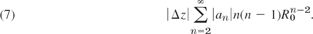
This series with an instead of |an| is the second derived series of (2) at z = R0 and converges absolutely by Theorem 3 of this section and Theorem 1 of Sec. 15.2. Hence our present series (7) converges. Let the sum of (7) (without the factor |Δz|) be K(R0). Since (6) is the right side of (5), our present result is

Letting Δz → 0 and noting that R0(< R) is arbitrary, we conclude that f(z) is analytic at any point interior to the circle of convergence and its derivative is represented by the derived series. From this the statements about the higher derivatives follow by induction.
Summary. The results in this section show that power series are about as nice as we could hope for: we can differentiate and integrate them term by term (Theorems 3 and 4). Theorem 5 accounts for the great importance of power series in complex analysis: the sum of such a series (with a positive radius of convergence) is an analytic function and has derivatives of all orders, which thus in turn are analytic functions. But this is only part of the story. In the next section we show that, conversely, every given analytic function f(z) can be represented by power series, called Taylor series and being the complex analog of the real Taylor series of calculus.
- Relation to Calculus. Material in this section generalizes calculus. Give details.
- Termwise addition. Write out the details of the proof on termwise addition and subtraction of power series.
- On Theorem 3. Prove that
 as n → ∞, as claimed.
 - Cauchy product. Show that

(a) by using the Cauchy product, (b) by differentiating a suitable series.
5–15 RADIUS OF CONVERGENCE BY DIFFERENTIATION OR INTEGRATION
Find the radius of convergence in two ways: (a) directly by the Cauchy–Hadamard formula in Sec. 15.2, and (b) from a series of simpler terms by using Theorem 3 or Theorem 4.
16–20 APPLICATIONS OF THE IDENTITY THEOREM
State clearly and explicitly where and how you are using Theorem 2.
- 16. Even functions. If f(z) in (2) is even (i.e., f(− z) = f(z)), show that an = 0 for odd n. Give examples.
- 17. Odd function. If f(z) in (2) is odd (i.e., f(−z) = −f(z)), show that an = 0 for even n. Give examples.
- 18. Binomial coefficients. Using (1 + z)p(1 + z)q = (1 + z)p + q, obtain the basic relation

- 19. Find applications of Theorem 2 in differential equations and elsewhere.
- 20. TEAM PROJECT. Fibonacci numbers.2 (a) The Fibonacci numbers are recursively defined by a0 = a1 = 1, an + 1 = an + an−1 if n = 1, 2, …. Find the limit of the sequence (an + 1/an).
(b) Fibonacci's rabbit problem. Compute a list of a1, …, a12. Show that a12 = 233 is the number of pairs of rabbits after 12 months if initially there is 1 pair and each pair generates 1 pair per month, beginning in the second month of existence (no deaths occurring).
(c) Generating function. Show that the generating function of the Fibonacci numbers is f(z) = 1/(1 − z − z2); that is, if a power series (1) represents this f(z), its coefficients must be the Fibonacci numbers and conversely. Hint. Start from f(z)(1 − z − z2) = 1 and use Theorem 2.
15.4 Taylor and Maclaurin Series
The Taylor series3 of a function f(z), the complex analog of the real Taylor series is

or, by (1), Sec. 14.4,
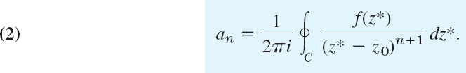
In (2) we integrate counterclockwise around a simple closed path C that contains z0 in its interior and is such that f(z) is analytic in a domain containing C and every point inside C.
A Maclaurin series3 is a Taylor series with center z0 = 0.
The remainder of the Taylor series (1) after the term an(z − z0)n is

(proof below). Writing out the corresponding partial sum of (1), we thus have

This is called Taylor's formula with remainder.
We see that Taylor series are power series. From the last section we know that power series represent analytic functions. And we now show that every analytic function can be represented by power series, namely, by Taylor series (with various centers). This makes Taylor series very important in complex analysis. Indeed, they are more fundamental in complex analysis than their real counterparts are in calculus.
Let f(z) be analytic in a domain D, and let z = z0 be any point in D. Then there exists precisely one Taylor series (1) with center z0 that represents f(z). This representation is valid in the largest open disk with center z0 in which f(z) is analytic. The remainders Rn(z) of (1) can be represented in the form (3). The coefficients satisfy the inequality
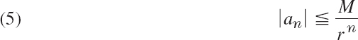
where M is the maximum of |f(z)| on a circle |z − z0| = r in D whose interior is also in D.
PROOF
The key tool is Cauchy's integral formula in Sec. 14.3; writing z and z* instead of z0 and z (so that z* is the variable of integration), we have

z lies inside C, for which we take a circle of radius r with center z0 and interior in D (Fig. 367). We develop 1/(z* − z) in (6) in powers of z − z0. By a standard algebraic manipulation (worth remembering!) we first have


For later use we note that since z* is on C while z is inside C, we have

To (7) we now apply the sum formula for a finite geometric sum

which we use in the form (take the last term to the other side and interchange sides)

Applying this with q = (z − z0)/(z* − z0) to the right side of (7), we get

We insert this into (6). Powers of z − z0 do not depend on the variable of integration z*, so that we may take them out from under the integral sign. This yields

with Rn(z) given by (3). The integrals are those in (2) related to the derivatives, so that we have proved the Taylor formula (4).
Since analytic functions have derivatives of all orders, we can take n in (4) as large as we please. If we let n approach infinity, we obtain (1). Clearly, (1) will converge and represent f(z) if and only if
![]()
We prove (9) as follows. Since z* lies on C, whereas z lies inside C (Fig. 367), we have |z* − z| > 0. Since f(z) is analytic inside and on C, it is bounded, and so is the function f(z*)/(z* − z), say,

for all z* on C. Also, C has the radius r = |z* − z0| and the length 2πr. Hence by the ML-inequality (Sec. 14.1) we obtain from (3)

Now |z − z0| < r because z lies inside C. Thus |z − z0|/r < 1, so that the right side approaches 0 as n → ∞. This proves that the Taylor series converges and has the sum f(z). Uniqueness follows from Theorem 2 in the last section. Finally, (5) follows from an in (1) and the Cauchy inequality in Sec. 14.4. This proves Taylor's theorem.
Accuracy of Approximation. We can achieve any preassinged accuracy in approximating f(z) by a partial sum of (1) by choosing n large enough. This is the practical use of formula (9).
Singularity, Radius of Convergence. On the circle of convergence of (1) there is at least one singular point of f(z), that is, a point z = c at which f(z) is not analytic (but such that every disk with center c contains points at which f(z) is analytic). We also say that f(z) is singular at c or has a singularity at c. Hence the radius of convergence R of (1) is usually equal to the distance from z0 to the nearest singular point of f(z).
(Sometimes R can be greater than that distance: Ln z is singular on the negative real axis, whose distance from z0 = −1 + i is 1, but the Taylor series of Ln z with center z0 = −1 + i has radius of convergence ![]() .)
.)
Power Series as Taylor Series
Taylor series are power series—of course! Conversely, we have
THEOREM 2 Relation to the Previous Section
A power series with a nonzero radius of convergence is thes Taylor series of its sum.
PROOF
Given the power series
![]()
Then f(z0) = a0. By Theorem 5 in Sec. 15.3 we obtain

and in general f(n)(z0) = n!an. With these coefficients the given series becomes the Taylor series of f(z) with center z0.
Comparison with Real Functions. One surprising property of complex analytic functions is that they have derivatives of all orders, and now we have discovered the other surprising property that they can always be represented by power series of the form (1). This is not true in general for real functions; there are real functions that have derivatives of all orders but cannot be represented by a power series. (Example: f(x) = exp(−1/x2) if x ≠ 0 and f(0) = 0; this function cannot be represented by a Maclaurin series in an open disk with center 0 because all its derivatives at 0 are zero.)
Important Special Taylor Series
These are as in calculus, with x replaced by complex z. Can you see why? (Answer. The coefficient formulas are the same.)
Let f(z) = 1/(1 − z). Then we have f(n)(z) = n!/(1 − z)n + 1, f(n)(0) = n!. Hence the Maclaurin expansion of 1/(1 − z) is the geometric series

f(z) is singular at z = 1; this point lies on the circle of convergence.
EXAMPLE 2 Exponential Function
We know that the exponential function ez (Sec. 13.5) is analytic for all z, and (ez)′ = ez. Hence from (1) with z0 = 0 we obtain the Maclaurin series

This series is also obtained if we replace x in the familiar Maclaurin series of ex by z.
Furthermore, by setting z = iy in (12) and separating the series into the real and imaginary parts (see Theorem 2, Sec. 15.1) we obtain
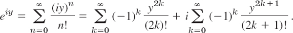
Since the series on the right are the familiar Maclaurin series of the real functions cos y and sin y, this shows that we have rediscovered the Euler formula

Indeed, one may use (12) for defining ez and derive from (12) the basic properties of ez. For instance, the differentiation formula (ez)′ = ez follows readily from (12) by termwise differentiation.
EXAMPLE 3 Trigonometric and Hyperbolic Functions
By substituting (12) into (1) of Sec. 13.6 we obtain

When z = x these are the familiar Maclaurin series of the real functions cos x and sin x. Similarly, by substituting (12) into (11), Sec. 13.6, we obtain
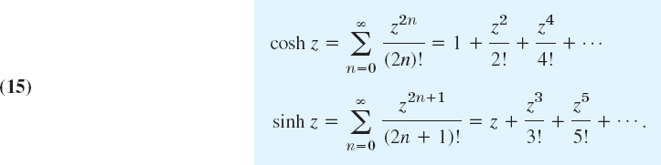
From (1) it follows that

Replacing z by −z and multiplying both sides by −1, we get

By adding both series we obtain

Practical Methods
The following examples show ways of obtaining Taylor series more quickly than by the use of the coefficient formulas. Regardless of the method used, the result will be the same. This follows from the uniqueness (see Theorem 1).
Find the Maclaurin series of f(z) = 1/(1 + z2).
Solution. By substituting −z2 for z in (11) we obtain

Find the Maclaurin series of f(z) = arctan z.
Solution. We have f′(z) = 1/(1 + z2). Integrating (19) term by term and using f(0) = 0 we get

this series represents the principal value of w = u + iv = arctan z defined as that value for which |u| < π/2.
EXAMPLE 7 Development by Using the Geometric Series
Develop 1/(c − z) in powers of z − z0, where c − z0 ≠ 0.
Solution. This was done in the proof of Theorem 1, where c = z*. The beginning was simple algebra and then the use of (11) with z replaced by (z − z0)/(c − z0):

This series converges for
EXAMPLE 8 Binomial Series, Reduction by Partial Fractions
Find the Taylor series of the following function with center z0 = 1.
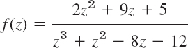
Solution. We develop f(z) in partial fractions and the first fraction in a binomial series
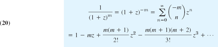
with m = 2 and the second fraction in a geometric series, and then add the two series term by term. This gives

We see that the first series converges for |z − 1| < 3 and the second for |z − 1| < 2. This had to be expected because 1/(z + 2)2 is singular at −2 and 2/(z − 3) at 3, and these points have distance 3 and 2, respectively, from the center z0 = 1. Hence the whole series converges for |z − 1| < 2.
- Calculus. Which of the series in this section have you discussed in calculus? What is new?
- On Examples 5 and 6. Give all the details in the derivation of the series in those examples.
3–10 MACLAURIN SERIES
Find the Maclaurin series and its radius of convergence.
- 3. sin 2z2
- 4.

- 5.

- 6.

- 7.

- 8. sin2z
- 9.

- 10.
11–14 HIGHER TRANSCENDENTAL FUNCTIONS
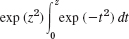
Find the Maclaurin series by termwise integrating the integrand. (The integrals cannot be evaluated by the usual methods of calculus. They define the error function erf z, sine integral Si(z), and Fresnel integrals4 S(z) and C(z), which occur in statistics, heat conduction, optics, and other applications. These are special so-called higher transcendental functions.)
- 11.

- 12.

- 13.

- 14.

- 15. CAS Project. sec, tan. (a) Euler numbers. The Maclaurin series
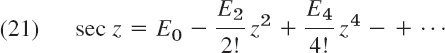
defines the Euler numbers E2n. Show that E0 = 1, E2 = −1, E4 = 5, E6 = −61. Write a program that computes the E2n from the coefficient formula in (1) or extracts them as a list from the series. (For tables see Ref. [GenRef1], p. 810, listed in App. 1.)
- (b) Bernoulli numbers. The Maclaurin series
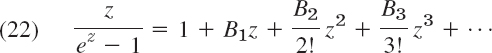
defines the Bernoulli numbers Bn. Using undetermined coefficients, show that

Write a program for computing Bn.
- (c) Tangent. Using (1), (2), Sec. 13.6, and (22), show that tan z has the following Maclaurin series and calculate from it a table of B0, …, B20:

- (b) Bernoulli numbers. The Maclaurin series
- 16. Inverse sine. Developing
 and integrating, show that

Show that this series represents the principal value of arcsin z (defined in Team Project 30, Sec. 13.7).
- 17. TEAM PROJECT. Properties from Maclaurin Series. Clearly, from series we can compute function values. In this project we show that properties of functions can often be discovered from their Taylor or Maclaurin series. Using suitable series, prove the following.
(a) The formulas for the derivatives of and ez, cos z, sin z, cosh z, sinh z. and Ln(1 + z)
(b)

(c) sin z ≠ 0 for all pure imaginary z = iy ≠ 0
18–25 TAYLOR SERIES
Find the Taylor series with center z0 and its radius of convergence.
- 18. 1/z, z0 = i
- 19. 1/(1 − z), z0 = i
- 20. cos2z, z0 = π/2
- 21. sin z, z0 = π/2
- 22. cosh (z − πi), z0 = πi
- 23. 1/(z + i)2, z0 = i
- 24. ez(z−2), z0 = 1
- 25. sinh (2z − i), z0 =i/2
15.5 Uniform Convergence. Optional
We know that power series are absolutely convergent (Sec. 15.2, Theorem 1) and, as another basic property, we now show that they are uniformly convergent. Since uniform convergence is of general importance, for instance, in connection with termwise integration of series, we shall discuss it quite thoroughly.
To define uniform convergence, we consider a series whose terms are any complex functions f0(z),f1(z), …

(This includes power series as a special case in which fm(z) = am(z − z0)m.) We assume that the series (1) converges for all z in some region G. We call its sum s(z) and its nth partial sum sn(z); thus
![]()
Convergence in G means the following. If we pick a z = z1 in G, then, by the definition of convergence at z1, for given ![]() > 0 we can find an N1(
> 0 we can find an N1(![]() ) such that
) such that
![]()
If we pick a z2 in G, keeping ![]() as before, we can find an N2(
as before, we can find an N2(![]() ) such that
) such that
![]()
and so on. Hence, given an ![]() > 0, to each z in G there corresponds a number Nz(
> 0, to each z in G there corresponds a number Nz(![]() ). This number tells us how many terms we need (what sn we need) at a z to make |s(z) − sn(z)| smaller than
). This number tells us how many terms we need (what sn we need) at a z to make |s(z) − sn(z)| smaller than ![]() . Thus this number Nz(
. Thus this number Nz(![]() ) measures the speed of convergence.
) measures the speed of convergence.
Small Nz(![]() ) means rapid convergence, large Nz(
) means rapid convergence, large Nz(![]() ) means slow convergence at the point z considered. Now, if we can find an N(
) means slow convergence at the point z considered. Now, if we can find an N(![]() ) larger than all these Nz(
) larger than all these Nz(![]() ) for all z in G, we say that the convergence of the series (1) in G is uniform. Hence this basic concept is defined as follows.
) for all z in G, we say that the convergence of the series (1) in G is uniform. Hence this basic concept is defined as follows.
DEFINITION Uniform Convergence
A series (1) with sum s(z) is called uniformly convergent in a region G if for every ![]() > 0 we can find an N = N(
> 0 we can find an N = N(![]() ), not depending on z, such that
), not depending on z, such that
![]()
Uniformity of convergence is thus a property that always refers to an infinite set in the z-plane, that is, a set consisting of infinitely many points.
Show that the geometric series 1 + z + z2 + … is (a) uniformly convergent in any closed disk |z| ![]() r < 1, (b) not uniformly convergent in its whole disk of convergence |z| < 1.
r < 1, (b) not uniformly convergent in its whole disk of convergence |z| < 1.
Solution. (a) For z in that closed disk we have |1 − z| ![]() 1 − r (sketch it). This implies that 1/|1 − z|
1 − r (sketch it). This implies that 1/|1 − z| ![]() 1/(1 − r). Hence (remember (8) in Sec. 15.4 with q = z)
1/(1 − r). Hence (remember (8) in Sec. 15.4 with q = z)

Since r < 1, we can make the right side as small as we want by choosing n large enough, and since the right side does not depend on z (in the closed disk considered), this means that the convergence is uniform.
(b) For given real K (no matter how large) and n we can always find a z in the disk |z| < 1 such that

simply by taking z close enough to 1. Hence no single N(![]() ) will suffice to make |s(z) − sn(z)| smaller than a given
) will suffice to make |s(z) − sn(z)| smaller than a given ![]() > 0 throughout the whole disk. By definition, this shows that the convergence of the geometric series in |z| < 1 is not uniform.
> 0 throughout the whole disk. By definition, this shows that the convergence of the geometric series in |z| < 1 is not uniform.
This example suggests that for a power series, the uniformity of convergence may at most be disturbed near the circle of convergence. This is true:
THEOREM 1 Uniform Convergence of Power Series
A power series

with a nonzero radius of convergence R is uniformly convergent in every circular disk |z − z0| ![]() r of radius r < R.
r of radius r < R.
PROOF
For |z − z0| ![]() r and any positive integers n and p we have
r and any positive integers n and p we have
![]()
Now (2) converges absolutely if |z − z0| = r < R (by Theorem 1 in Sec. 15.2). Hence it follows from the Cauchy convergence principle (Sec. 15.1) that, an ![]() > 0 being given, we can find an N(
> 0 being given, we can find an N(![]() ) such that
) such that
![]()
From this and (3) we obtain
![]()
for all z in the disk |z − z0| ![]() r, every n > N(
r, every n > N(![]() ), and every p = 1, 2, …. Since N(
), and every p = 1, 2, …. Since N(![]() ) is independent of z, this shows uniform convergence, and the theorem is proved.
) is independent of z, this shows uniform convergence, and the theorem is proved.
Thus we have established uniform convergence of power series, the basic concern of this section. We now shift from power series to arbitary series of variable terms and examine uniform convergence in this more general setting. This will give a deeper understanding of uniform convergence.
Properties of Uniformly Convergent Series
Uniform convergence derives its main importance from two facts:
1. If a series of continuous terms is uniformly convergent, its sum is also continuous (Theorem 2, below).
2. Under the same assumptions, termwise integration is permissible (Theorem 3). This raises two questions:
1. How can a converging series of continuous terms manage to have a discontinuous sum? (Example 2)
2. How can something go wrong in termwise integration? (Example 3) Another natural question is:
3. What is the relation between absolute convergence and uniform convergence? The surprising answer: none. (Example 5)
These are the ideas we shall discuss.
If we add finitely many continuous functions, we get a continuous function as their sum. Example 2 will show that this is no longer true for an infinite series, even if it converges absolutely. However, if it converges uniformly, this cannot happen, as follows.
THEOREM 2 Continuity of the Sum
Let the series

be uniformly convergent in a region G. Let F(z) be its sum. Then if each term fm(z) is continuous at a point z1 in G, the function F(z) is continuous at z1.
PROOF
Let sn(z) be the nth partial sum of the series and Rn(z) the corresponding remainder:
![]()
Since the series converges uniformly, for a given ![]() > 0 we can find an N = N(
> 0 we can find an N = N(![]() ) such that
) such that
![]()
Since sN(z) is a sum of finitely many functions that are continuous at z1, this sum is continuous at z1. Therefore, we can find δ > 0 a such that
![]()
Using F = sN + RN and the triangle inequality (Sec. 13.2), for these z we thus obtain

This implies that F(z) is continuous at z1, and the theorem is proved.
EXAMPLE 2 Series of Continuous Terms with a Discontinuous Sum
Consider the series

This is a geometric series with q = 1/(1 + x2) times a factor x2. Its nth partial sum is

We now use the trick by which one finds the sum of a geometric series, namely, we multiply sn(x) by −q = −1/(1 + x2),

Adding this to the previous formula, simplifying on the left, and canceling most terms on the right, we obtain

thus

The exciting Fig. 368 “explains” what is going on. We see that if x ≠ 0, the sum is
![]()
but for x = 0 we have sn(0) = 1 − 1 = 0 for all n, hence s(0) = 0. So we have the surprising fact that the sum is discontinuous (at x = 0), although all the terms are continuous and the series converges even absolutely (its terms are nonnegative, thus equal to their absolute value!).
Theorem 2 now tells us that the convergence cannot be uniform in an interval containing x = 0. We can also verify this directly. Indeed, for x ≠ 0 the remainder has the absolute value

and we see that for a given ![]() (< 1) we cannot find an N depending only on
(< 1) we cannot find an N depending only on ![]() such that |Rn| <
such that |Rn| < ![]() for all n > N(
for all n > N(![]() ) and all x, say, in the interval 0
) and all x, say, in the interval 0 ![]() x
x ![]() 1.
1.

Fig. 368. Partial sums in Example 2
Termwise Integration
This is our second topic in connection with uniform convergence, and we begin with an example to become aware of the danger of just blindly integrating term-by-term.
EXAMPLE 3 Series for Which Termwise Integration Is Not Permissible
Let um(x) = mxe−mx2 and consider the series

in the interval 0 ![]() x
x ![]() 1. The nth partial sum is
1. The nth partial sum is
![]()
Hence the series has the sum ![]() (0
(0 ![]() x
x ![]() 1). From this we obtain
1). From this we obtain

On the other hand, by integrating term by term and using f1 + f2 + … + fn = sn, we have

Now sn = un and the expression on the right becomes
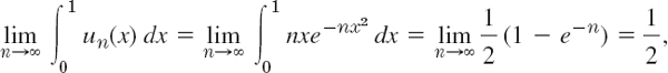
but not 0. This shows that the series under consideration cannot be integrated term by term from x = 0 to x = 1.
The series in Example 3 is not uniformly convergent in the interval of integration, and we shall now prove that in the case of a uniformly convergent series of continuous functions we may integrate term by term.
THEOREM 3 Termwise Integration
Let

be a uniformly convergent series of continuous functions in a region G. Let C be any path in G. Then the series

is convergent and has the sum ∫C F(z) dz.
PROOF
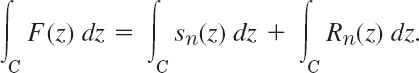
From Theorem 2 it follows that F(z) is continuous. Let sn(z) be the nth partial sum of the given series and Rn(z) the corresponding remainder. Then F = sn + Rn and by integration,
Let L be the length of C. Since the given series converges uniformly, for every given ![]() > 0 we can find a number N such that |Rn(z)| <
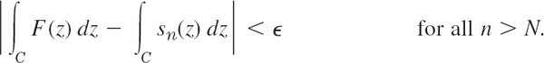
> 0 we can find a number N such that |Rn(z)| < ![]() /L for all n > N and all z in G. By applying the ML-inequality (Sec. 14.1) we thus obtain
/L for all n > N and all z in G. By applying the ML-inequality (Sec. 14.1) we thus obtain

Since Rn = F − sn, this means that
Hence, the series (4) converges and has the sum indicated in the theorem.
Theorems 2 and 3 characterize the two most important properties of uniformly convergent series. Also, since differentiation and integration are inverse processes, Theorem 3 implies
THEOREM 4 Termwise Differentiation
Let the series f0(z) + f1(z) + f2(z) + … be convergent in a region G and let F(z) be its sum. Suppose that the series ![]() converges uniformly in G and its terms are continuous in G. Then
converges uniformly in G and its terms are continuous in G. Then
![]()
Test for Uniform Convergence
Uniform convergence is usually proved by the following comparison test.
THEOREM 5 Weierstrass5 M-Test for Uniform Convergence
Consider a series of the form (1) in a region G of the z-plane. Suppose that one can find a convergent series of constant terms,
![]()
such that |fm(z)| ![]() Mm for all z in G and every m = 0, 1, …. Then (1) is uniformly convergent in G.
Mm for all z in G and every m = 0, 1, …. Then (1) is uniformly convergent in G.
The simple proof is left to the student (Team Project 18).
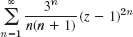
Does the following series converge uniformly in the disk |z| ![]() 1?
1?

Solution. Uniform convergence follows by the Weierstrass M-test and the convergence of Σ1/m2 (see Sec. 15.1, in the proof of Theorem 8) because

No Relation Between Absolute and Uniform Convergence
We finally show the surprising fact that there are series that converge absolutely but not uniformly, and others that converge uniformly but not absolutely, so that there is no relation between the two concepts.
EXAMPLE 5 No Relation Between Absolute and Uniform Convergence
The series in Example 2 converges absolutely but not uniformly, as we have shown. On the other hand, the series

converges uniformly on the whole real line but not absolutely.
Proof. By the familiar Leibniz test of calculus (see App. A3.3) the remainder Rn does not exceed its first term in absolute value, since we have a series of alternating terms whose absolute values form a monotone decreasing sequence with limit zero. Hence given ![]() > 0, for all x we have
> 0, for all x we have

This proves uniform convergence, since N(![]() ) does not depend on x.
) does not depend on x.
The convergence is not absolute because for any fixed x we have

where k is a suitable constant, and kΣ1/m diverges.
- CAS EXPERIMENT. Graphs of Partial Sums. (a) Fig. 368. Produce this exciting figure using your CAS. Add further curves, say, those of s256, s1024, etc. on the same screen.
- (b) Power series. Study the nonuniformity of convergence experimentally by graphing partial sums near the endpoints of the convergence interval for real z = x.
Where does the power series converge uniformly? Give reason.
- 2.

- 3.

- 4.

- 5.

- 6.

- 7.

- 8.
- 9.

10–17 UNIFORM CONVERGENCE
Prove that the series converges uniformly in the indicated region.
- 10.

- 11.

- 12.

- 13.

- 14.

- 15.

- 16.

- 17.

- 18. TEAM PROJECT. Uniform Convergence.
(a) Weierstrass M-test. Give a proof.
(b) Termwise differentiation. Derive Theorem 4 from Theorem 3.
(c) Subregions. Prove that uniform convergence of a series in a region G implies uniform convergence in any portion of G. Is the converse true?
(d) Example 2. Find the precise region of convergence of the series in Example 2 with x replaced by a complex variable z.
(e) Figure 369. Show that
 if x ≠ 0 and 0 if x = 0. Verify by computation that the partial sums s1, s2, s3 look as shown in Fig. 369.
19–20 HEAT EQUATION
Show that (9) in Sec. 12.6 with coefficients (10) is a solution of the heat equation for t > 0, assuming that f(x) is continuous on the interval 0 ![]() x
x ![]() L and has one-sided derivatives at all interior points of that interval. Proceed as follows.
L and has one-sided derivatives at all interior points of that interval. Proceed as follows.
- 19. Show that |Bn| is bounded, say |Bn| < K for all n. Conclude that

and, by the Weierstrass test, the series (9) converges uniformly with respect to x and t for t
 t0, 0 x L. Using Theorem 2, show that u(x, t) is continuous for t t0 and thus satisfies the boundary conditions (2) for t t0.
 - 20. Show that
 if t t0 and the series of the expressions on the right converges, by the ratio test. Conclude from this, the Weierstrass test, and Theorem 4 that the series (9) can be differentiated term by term with respect to t and the resulting series has the sum ∂u/∂t. Show that (9) can be differentiated twice with respect to x and the resulting series has the sum ∂2u/∂x2. Conclude from this and the result to Prob. 19 that (9) is a solution of the heat equation for all t t0. (The proof that (9) satisfies the given initial condition can be found in Ref. [C10] listed in App. 1.)
CHAPTER 15 REVIEW QUESTIONS AND PROBLEMS
- What is convergence test for series? State two tests from memory. Give examples.
- What is a power series? Why are these series very important in complex analysis?
- What is absolute convergence? Conditional convergence? Uniform convergence?
- What do you know about convergence of power series?
- What is a Taylor series? Give some basic examples.
- What do you know about adding and multiplying power series?
- Does every function have a Taylor series development? Explain.
- Can properties of functions be discovered from Maclaurin series? Give examples.
- What do you know about termwise integration of series?
- How did we obtain Taylor's formula from Cauchy's formula?
11–15 RADIUS OF CONVERGENCE
Find the radius of convergence.
- 11.

- 12.

- 13.
- 14.

- 15.

16–20 RADIUS OF CONVERGENCE
Find the radius of convergence. Try to identify the sum of the series as a familiar function.
- 16.

- 17.

- 18.

- 19.

- 20.

21–25 MACLAURIN SERIES
Find the Maclaurin series and its radius of convergence. Show details.
- 21. (sinh z2)/z2
- 22. 1/(1 − z)3
- 23. cos2z
- 24. 1/(πz + 1)
- 25. −(exp/(−z2)−1)/z2
26–30 TAYLOR SERIES
Find the Taylor series with the given point as center and its radius of convergence.
- 26. z4, i
- 27. cosz,
 π
π - 28. 1/z, 2i
- 29. Ln z, 3
- 30. ez, πi
SUMMARY OF CHAPTER 15 Power Series, Taylor Series
Sequences, series, and convergence tests are discussed in Sec. 15.1. A power series is of the form (Sec. 15.2)

z0 is its center. The series (1) converges for |z − z0| < R and diverges for |z − z0| > R, where R is the radius of convergence. Some power series converge for all z (then we write R = ∞). In exceptional cases a power series may converge only at the center; such a series is practically useless. Also, R = lim |an/an + 1| if this limit exists. The series (1) converges absolutely (Sec. 15.2) and uniformly (Sec. 15.5) in every closed disk |z − z0| ![]() r < R (R > 0). It represents an analytic function f(z) for |z − z0| < R. The derivatives f′(z),f″(z), … are obtained by termwise differentiation of (1), and these series have the same radius of convergence R as (1). See Sec. 15.3.
r < R (R > 0). It represents an analytic function f(z) for |z − z0| < R. The derivatives f′(z),f″(z), … are obtained by termwise differentiation of (1), and these series have the same radius of convergence R as (1). See Sec. 15.3.
Conversely, every analytic function f(z) can be represented by power series. These Taylor series of f(z) are of the form (Sec. 15.4)

as in calculus. They converge for all z in the open disk with center z0 and radius generally equal to the distance from z0 to the nearest singularity of f(z) (point at which f(z) ceases to be analytic as defined in Sec. 15.4). If f(z) is entire (analytic for all z; see Sec. 13.5), then (2) converges for all z. The functions ez, cos z, sin z, etc. have Maclaurin series, that is, Taylor series with center 0, similar to those in calculus (Sec. 15.4).
1Named after the French mathematicians A. L. CAUCHY (see Sec. 2.5) and JACQUES HADAMARD (1865–1963). Hadamard made basic contributions to the theory of power series and devoted his lifework to partial differential equations.
2LEONARDO OF PISA, called FIBONACCI (= son of Bonaccio), about 1180–1250, Italian mathematician, credited with the first renaissance of mathematics on Christian soil.
3BROOK TAYLOR (1685–1731), English mathematician who introduced real Taylor series. COLIN MACLAURIN (1698–1746), Scots mathematician, professor at Edinburgh.
4AUGUSTIN FRESNEL (1788–1827), French physicist and engineer, known for his work in optics.
5KARL WEIERSTRASS (1815–1897), great German mathematician, who developed complex analysis based on the concept of power series and residue integration. (See footnote in Section 13.4.) He put analysis on a sound theoretical footing. His mathematical rigor is so legendary that one speaks Weierstrassian rigor. (See paper by Birkhoff and Kreyszig, 1984 in footnote in Sec. 5.5; Kreyszig, E., On the Calculus, of Variations and Its Major Influences on the Mathematics of the First Half of Our Century. Part II, American Mathematical Monthly (1994), 101, No. 9, pp. 902–908). Weierstrass also made contributions to the calculus of variations, approximation theory, and differential geometry. He obtained the concept of uniform convergence in 1841 (published 1894, sic!); the first publication on the concept was by G. G. STOKES (see Sec 10.9) in 1847.