
CHAPTER 16
Laurent Series. Residue Integration

The main purpose of this chapter is to learn about another powerful method for evaluating complex integrals and certain real integrals. It is called residue integration. Recall that the first method of evaluating complex integrals consisted of directly applying Cauchy's integral formula of Sec. 14.3. Then we learned about Taylor series (Chap. 15) and will now generalize Taylor series. The beauty of residue integration, the second method of integration, is that it brings together a lot of the previous material.
Laurent series generalize Taylor series. Indeed, whereas a Taylor series has positive integer powers (and a constant term) and converges in a disk, a Laurent series (Sec. 16.1) is a series of positive and negative integer powers of z − z0 and converges in an annulus (a circular ring) with center z0. Hence, by a Laurent series, we can represent a given function f(z) that is analytic in an annulus and may have singularities outside the ring as well as in the “hole” of the annulus.
We know that for a given function the Taylor series with a given center z0 is unique. We shall see that, in contrast, a function f(z) can have several Laurent series with the same center z0 and valid in several concentric annuli. The most important of these series is the one that converges for 0 < |z − z0| < R, that is, everywhere near the center z0 except at z0 itself, where z0 is a singular point of f(z). The series (or finite sum) of the negative powers of this Laurent series is called the principal part of the singularity of f(z) at z0, and is used to classify this singularity (Sec. 16.2). The coefficient of the power 1/(z − z0) of this series is called the residue of f(z) at z0. Residues are used in an elegant and powerful integration method, called residue integration, for complex contour integrals (Sec. 16.3) as well as for certain complicated real integrals (Sec. 16.4).
Prerequisite: Chaps. 13, 14, Sec. 15.2.
Sections that may be omitted in a shorter course:16.2, 16.4.
References and Answers to Problems: App. 1 Part D, App. 2.
16.1 Laurent Series
Laurent series generalize Taylor series. If, in an application, we want to develop a function f(z) in powers of z − z0 when f(z) is singular at z0 (as defined in Sec. 15.4), we cannot use a Taylor series. Instead we can use a new kind of series, called Laurent series,1 consisting of positive integer powers of z − z0 (and a constant) as well as negative integer powers of z − z0; this is the new feature.
Laurent series are also used for classifying singularities (Sec. 16.2) and in a powerful integration method (“residue integration,” Sec. 16.3).
A Laurent series of f(z) converges in an annulus (in the “hole” of which f(z) may have singularities), as follows.
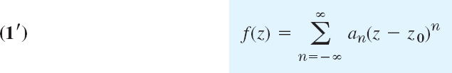
Let f(z) be analytic in a domain containing two concentric circles C1 and C2 with center z0 and the annulus between them (blue in Fig. 370). Then f(z) can be represented by the Laurent series

consisting of nonnegative and negative powers. The coefficients of this Laurent series are given by the integrals

taken counterclockwise around any simple closed path C that lies in the annulus and encircles the inner circle, as in Fig. 370. [The variable of integration is denoted by z* since z is used in (1).]
This series converges and represents f(z) in the enlarged open annulus obtained from the given annulus by continuously increasing the outer circle C1 and decreasing C2 until each of the two circles reaches a point where f(z) is singular.
In the important special case that z0 is the only singular point of f(z) inside C2, this circle can be shrunk to the point z0, giving convergence in a disk except at the center. In this case the series (or finite sum) of the negative powers of (1) is called the principal part of f(z) at z0 [or of that Laurent series (1)].

where all the coefficients are now given by a single integral formula, namely,

Let us now prove Laurent's theorem.
PROOF
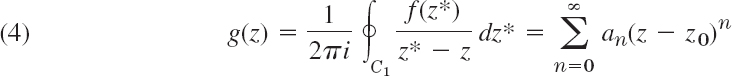
(a) The nonnegative powers are those of a Taylor series.
To see this, we use Cauchy's integral formula (3) in Sec. 14.3 with z* (instead of z) as the variable of integration and z instead of z0. Let g(z) and h(z) denote the functions represented by the two terms in (3), Sec. 14.3. Then

Here z is any point in the given annulus and we integrate counterclockwise over both C1 and C2, so that the minus sign appears since in (3) of Sec. 14.3 the integration over C2 is taken clockwise. We transform each of these two integrals as in Sec. 15.4. The first integral is precisely as in Sec. 15.4. Hence we get exactly the same result, namely, the Taylor series of g(z),
with coefficients [see (2), Sec. 15.4, counterclockwise integration]

Here we can replace C1 by C (see Fig. 370), by the principle of deformation of path, since z0, the point where the integrand in (5) is not analytic, is not a point of the annulus. This proves the formula for the an in (2).
(b) The negative powers in (1) and the formula for bn in (2) are obtained if we consider h(z). It consists of the second integral times −1/(2πi) in (3). Since z lies in the annulus, it lies in the exterior of the path C2. Hence the situation differs from that for the first integral. The essential point is that instead of [see in Sec. 15.4]

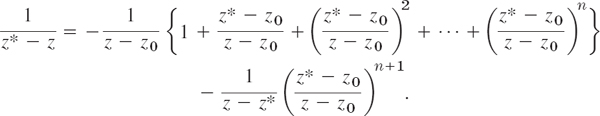
Consequently, we must develop the expression 1/(z* − z) in the integrand of the second integral in (3) in powers of (z* − z0)/(z − z0) (instead of the reciprocal of this) to get a convergent series. We find

Compare this for a moment with (7) in Sec. 15.4, to really understand the difference. Then go on and apply formula (8), Sec. 15.4, for a finite geometric sum, obtaining
Multiplication by −f(z*)/2πi and integration over C2 on both sides now yield

with the last term on the right given by

As before, we can integrate over C instead of C2 in the integrals on the right. We see that on the right, the power 1/(z − z0)n is multiplied by bn as given in (2). This establishes Laurent's theorem, provided
![]()
(c) Convergence proof of (8). Very often (1) will have only finitely many negative powers. Then there is nothing to be proved. Otherwise, we begin by noting that f(z*)/(z − z*) in (7) is bounded in absolute value, say,

because f(z*) is analytic in the annulus and on C2, and z* lies on C2 and z outside, so that z − z* ≠ 0. From this and the ML-inequality (Sec. 14.1) applied to (7) we get the inequality (L = 2πr2 = length of C2, r2 = |z* −z0| = radius of C2 = const)
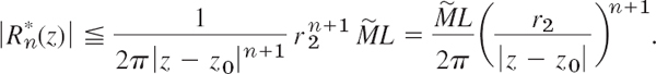
From (6b) we see that the expression on the right approaches zero as n approaches infinity. This proves (8). The representation (1) with coefficients (2) is now established in the given annulus.
(d) Convergence of (1) in the enlarged annulus. The first series in (1) is a Taylor series [representing g(z)]; hence it converges in the disk D with center z0 whose radius equals the distance of the singularity (or singularities) closest to z0. Also, g(z) must be singular at all points outside C1 where f(z) is singular.
The second series in (1), representing h(z), is a power series in Z = 1/(z − z0). Let the given annulus be r2 < |z − z0| < r1, where r1 and r2 are the radii of C1 and C2, respectively (Fig. 370). This corresponds to 1/r2 > |Z| > 1/r1. Hence this power series in Z must converge at least in the disk |Z| < 1/r2. This corresponds to the exterior |z − z0| > r2 of C2, so that h(z) is analytic for all z outside C2. Also, h(z) must be singular inside C2 where f(z) is singular, and the series of the negative powers of (1) converges for all z in the exterior E of the circle with center z0 and radius equal to the maximum distance from z0 to the singularities of f(z) inside C2. The domain common to D and E is the enlarged open annulus characterized near the end of Laurent's theorem, whose proof is now complete.
Uniqueness. The Laurent series of a given analytic function f(z), in its annulus of convergence is unique (see Team Project 18). However, f(z) may have different Laurent series in two annuli with the same center; see the examples below. The uniqueness is essential. As for a Taylor series, to obtain the coefficients of Laurent series, we do not generally use the integral formulas (2); instead, we use various other methods, some of which we shall illustrate in our examples. If a Laurent series has been found by any such process, the uniqueness guarantees that it must be the Laurent series of the given function in the given annulus.
EXAMPLE 1 Use of Maclaurin Series
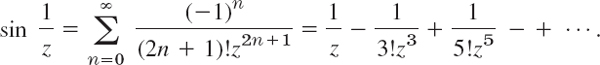
Find the Laurent series of z−5 sin z with center 0.
Solution. By (14), Sec. 15.4, we obtain
![]()
Here the “annulus” of convergence is the whole complex plane without the origin and the principal part of the series at 0 is ![]()
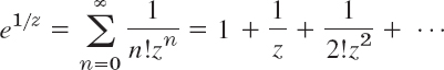
Find the Laurent series of z2e1/z with center 0.
Solution. From (12) in Sec. 15.4 with z replaced by 1/z we obtain a Laurent series whose principal part is an infinite series,
![]()
EXAMPLE 3 Development of 1/(1 − z)
Develop 1/(1 − z) (a) in nonnegative powers of z, (b) in negative powers of z.
Solution.


EXAMPLE 4 Laurent Expansions in Different Concentric Annuli
Find all Laurent series of 1/(z3 − z4) with center 0.
Solution. Multiplying by 1/z3, we get from Example 3


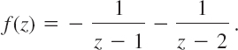
EXAMPLE 5 Use of Partial Fractions
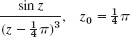
Find all Taylor and Laurent series of ![]() with center 0.
with center 0.
Solution. In terms of partial fractions,
(a) and (b) in Example 3 take care of the first fraction. For the second fraction,


(I) From (a) and (c), valid for |z| < 1 (see Fig. 371),
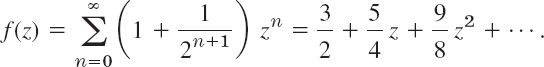
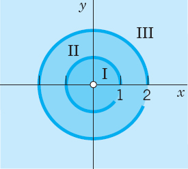
Fig. 371. Regions of convergence in Example 5
(II) From (c) and (b), valid for 1 < |z| < 2
![]()
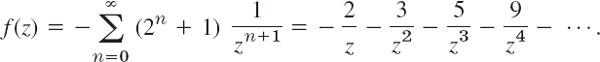
(III) From (d) and (b), valid for |z| > 2,
If f(z) in Laurent's theorem is analytic inside C2, the coefficients bn in (2) are zero by Cauchy's integral theorem, so that the Laurent series reduces to a Taylor series. Examples 3(a) and 5(I) illustrate this.
1–8 LAURENT SERIES NEAR A SINGULARITY AT 0
Expand the function in a Laurent series that converges for 0 < |z| < R and determine the precise region of convergence. Show the details of your work.
9–16 LAURENT SERIES NEAR A SINGULARITY AT z0
Find the Laurent series that converges for 0 < |z − z0| < R and determine the precise region of convergence. Show details.
- 9.

- 10.

- 11.

- 12.

- 13.

- 14.

- 15.

- 16.
- 17. CAS PROJECT. Partial Fractions. Write a program for obtaining Laurent series by the use of partial fractions. Using the program, verify the calculations in Example 5 of the text. Apply the program to two other functions of your choice.
- 18. TEAM PROJECT. Laurent Series. (a) Uniqueness. Prove that the Laurent expansion of a given analytic function in a given annulus is unique.
(b) Accumulation of singularities. Does tan (1/z) have a Laurent series that converges in a region 0 < |z| < R? (Give a reason.)
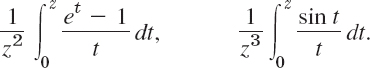
(c) Integrals. Expand the following functions in a Laurent series that converges for |z| > 0:
19–25 TAYLOR AND LAURENT SERIES
Find all Taylor and Laurent series with center z0. Determine the precise regions of convergence. Show details.
- 19.

- 20.

- 21.

- 22.

- 23.

- 24.

- 25.
16.2 Singularities and Zeros. Infinity
Roughly, a singular point of an analytic function f(z) is a z0 at which f(z) ceases to be analytic, and a zero is a z at which f(z) = 0. Precise definitions follow below. In this section we show that Laurent series can be used for classifying singularities and Taylor series for discussing zeros.
Singularities were defined in Sec. 15.4, as we shall now recall and extend. We also remember that, by definition, a function is a single-valued relation, as was emphasized in Sec. 13.3.
We say that a function f(z) is singular or has a singularity at a point z = z0 if f(z) is not analytic (perhaps not even defined) at z = z0, but every neighborhood of z = z0 contains points at which f(z) is analytic. We also say that z = z0 is a singular point of f(z).
We call z = z0 an isolated singularity of f(z) if z = z0 has a neighborhood without further singularities of f(z). Example: tan z has isolated singularities at ±π/2, ±3π/2, etc.; tan (1/z) has a nonisolated singularity at 0. (Explain!)
Isolated singularities of f(z) at z = z0 can be classified by the Laurent series

valid in the immediate neighborhood of the singular point z = z0, except at z0 itself, that is, in a region of the form
![]()
The sum of the first series is analytic at z = z0, as we know from the last section. The second series, containing the negative powers, is called the principal part of (1), as we remember from the last section. If it has only finitely many terms, it is of the form

Then the singularity of f(z) at z = z0 is called a pole, and m is called its order. Poles of the first order are also known as simple poles.
If the principal part of (1) has infinitely many terms, we say that f(z) has at z = z0 an isolated essential singularity.
We leave aside nonisolated singularities.
EXAMPLE 1 Poles. Essential Singularities
The function

has a simple pole at z = 0 and a pole of fifth order at z = 2. Examples of functions having an isolated essential singularity at z = 0 are
Section 16.1 provides further examples. In that section, Example 1 shows that z−5 sin z has a fourth-order pole at 0. Furthermore, Example 4 shows that 1/(z3 − z4) has a third-order pole at 0 and a Laurent series with infinitely many negative powers. This is no contradiction, since this series is valid for |z| > 1; it merely tells us that in classifying singularities it is quite important to consider the Laurent series valid in the immediate neighborhood of a singular point. In Example 4 this is the series (I), which has three negative powers.
The classification of singularities into poles and essential singularities is not merely a formal matter, because the behavior of an analytic function in a neighborhood of an essential singularity is entirely different from that in the neighborhood of a pole.
EXAMPLE 2 Behavior Near a Pole
f(z) = 1/z2 has a pole at z = 0, and |f(z)| → ∞ as z → 0 in any manner. This illustrates the following theorem.
If f(z) is analytic and has a pole at z = z0, then |f(z)| → ∞ as z → z0 in any manner.
The proof is left as an exercise (see Prob. 24).
EXAMPLE 3 Behavior Near an Essential Singularity
The function f(z) = e1/z has an essential singularity at z = 0. It has no limit for approach along the imaginary axis; it becomes infinite if z → 0 through positive real values, but it approaches zero if z → 0 through negative real values. It takes on any given value c = c0ei∞ ≠ 0 in an arbitrarily small ![]() -neighborhood of z = 0. To see the latter, we set z = reiθ, and then obtain the following complex equation for r and θ, which we must solve:
-neighborhood of z = 0. To see the latter, we set z = reiθ, and then obtain the following complex equation for r and θ, which we must solve:
![]()
Equating the absolute values and the arguments, we have e(cos θ)/r = c0, that is
![]()
respectively. From these two equations and cos2 θ + sin2θ = r2(ln c0)2 + α2r2 = 1 we obtain the formulas
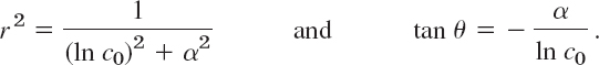
Hence r can be made arbitrarily small by adding multiples of 2π to α, leaving c unaltered. This illustrates the very famous Picard's theorem (with z = 0 as the exceptional value).
If f(z) is analytic and has an isolated essential singularity at a point z0, it takes on every value, with at most one exceptional value, in an arbitrarily small ![]() -neighborhood of z0.
-neighborhood of z0.
For the rather complicated proof, see Ref. [D4], vol. 2, p. 258. For historical information on Picard, see footnote 9 in Problem Set 1.7.
Removable Singularities. We say that a function f(z) has a removable singularity at z = z0 if f(z) is not analytic at z = z0, but can be made analytic there by assigning a suitable value f(z0). Such singularities are of no interest since they can be removed as just indicated. Example: f(z) = (sin z)/z becomes analytic at z = 0 if we define f(0) = 1.
Zeros of Analytic Functions
A zero of an analytic function f(z) in a domain D is a z = z0 in D such that f(z0) = 0. A zero has order n if not only f but also the derivatives f′, f″, …. f(n−1) are all 0 at z = z0 but f(n)(z0) ≠ 0. A first-order zero is also called a simple zero. For a second-order zero, f(z0) = f′(z0) = 0 but f″(z0) ≠ 0. And so on.
The function 1 + z2 has simple zeros at ±i. The function (1 − z4)2 has second-order zeros at ±1 and ±i. The function (z − a)3 has a third-order zero at z = a. The function ez has no zeros (see Sec. 13.5). The function sin z has simple zeros at 0, ±π, ±2π, …, and sin2z has second-order zeros at these points. The function 1 − cos z has second-order zeros at 0, ±2π, ±4π, …, and the function (1 − cos z)2 has fourth-order zeros at these points.
Taylor Series at a Zero. At an nth-order zero z = z0 of f(z), the derivatives f′(z0), …, f(n−1)(z0) are zero, by definition. Hence the first few coefficients a0, …, an−1 of the Taylor series (1), Sec. 15.4, are zero, too, whereas an ≠ 0, so that this series takes the form

This is characteristic of such a zero, because, if f(z) has such a Taylor series, it has an nth-order zero at z = z0, as follows by differentiation.
Whereas nonisolated singularities may occur, for zeros we have
The zeros of an analytic function f(z)(![]() 0) are isolated; that is, each of them has a neighborhood that contains no further zeros of f(z)
0) are isolated; that is, each of them has a neighborhood that contains no further zeros of f(z)
PROOF
The factor (z − z0)n in (3) is zero only at z = z0. The power series in the brackets […] represents an analytic function (by Theorem 5 in Sec. 15.3), call it g(z). Now g(z0) = an ≠ 0, since an analytic function is continuous, and because of this continuity, also g(z) ≠ 0 in some neighborhood of z = z0. Hence the same holds of f(z).
This theorem is illustrated by the functions in Example 4.
Poles are often caused by zeros in the denominator. (Example: tan z has poles where cos z is zero.) This is a major reason for the importance of zeros. The key to the connection is the following theorem, whose proof follows from (3) (see Team Project 12).
Let f(z) be analytic at z = z0 and have a zero of nth order at z = z0. Then 1/f(z) has a pole of nth order at z = z0; and so does h(z)/f(z), provided h(z) is analytic at z = z0 and h(z0) ≠ 0.

Riemann Sphere. Point at Infinity
When we want to study complex functions for large |z|, the complex plane will generally become rather inconvenient. Then it may be better to use a representation of complex numbers on the so-called Riemann sphere. This is a sphere S of diameter 1 touching the complex z-plane at z = 0 (Fig. 372), and we let the image of a point P (a number z in the plane) be the intersection P* of the segment PN with S, where N is the “North Pole” diametrically opposite to the origin in the plane. Then to each z there corresponds a point on S.
Conversely, each point on S represents a complex number z, except for N, which does not correspond to any point in the complex plane. This suggests that we introduce an additional point, called the point at infinity and denoted ∞ (“infinity”) and let its image be N. The complex plane together with ∞ is called the extended complex plane. The complex plane is often called the finite complex plane, for distinction, or simply the complex plane as before. The sphere S is called the Riemann sphere. The mapping of the extended complex plane onto the sphere is known as a stereographic projection. (What is the image of the Northern Hemisphere? Of the Western Hemisphere? Of a straight line through the origin?)
Analytic or Singular at Infinity
If we want to investigate a function f(z) for large |z|, we may now set z = 1/w and investigate f(z) = f(1/w) ≡ g(w) in a neighborhood of w = 0. We define f(z) to be analytic or singular at infinity if g(w) is analytic or singular, respectively, at w = 0. We also define
![]()
if this limit exists.
Furthermore, we say that f(z) has an nth-order zero at infinity if f(1/w) has such a zero at w = 0. Similarly for poles and essential singularities.
EXAMPLE 5 Functions Analytic or Singular at Infinity. Entire and Meromorphic Functions
The function f(z) = 1/z2 is analytic at ∞ since g(w) = f(w) = w2 is analytic at w = 0, and f(z) has a second-order zero at ∞. The function f(z) = z3 is singular at ∞ and has a third-order pole there since the function g(w) = f(1/w) = 1/w3 has such a pole at w = 0. The function ez has an essential singularity at ∞ since e1/w has such a singularity at w = 0. Similarly, cos z and sin z have an essential singularity at ∞.
Recall that an entire function is one that is analytic everywhere in the (finite) complex plane. Liouville's theorem (Sec. 14.4) tells us that the only bounded entire functions are the constants, hence any nonconstant entire function must be unbounded. Hence it has a singularity at ∞, a pole if it is a polynomial or an essential singularity if it is not. The functions just considered are typical in this respect.
An analytic function whose only singularities in the finite plane are poles is called a meromorphic function. Examples are rational functions with nonconstant denominator, tan z, cot z, sec z, and csc z.
In this section we used Laurent series for investigating singularities. In the next section we shall use these series for an elegant integration method.
1–10 ZEROS
Determine the location and order of the zeros.

- (z4 − 81)3
- (z + 81i)4
- tan22z
- z−2sin2πz
- cosh4z
- z4 + (1 − 8i)z2 − 8i
- (sin z − 1)3
- sin 2z cos 2z
- (z2 − 8)3(exp(z2) − 1)
- Zeros. If f(z) is analytic and has a zero of order n at z = z0, show that f2(z) has a zero of order 2n at z0.
- TEAM PROJECT. Zeros. (a) Derivative. Show that if f(z) has a zero of order n > 1 at z = z0, then f′(z) has a zero of order n − 1 at z0.
- (b) Poles and zeros. Prove Theorem 4.
- (c) Isolated k-points. Show that the points at which a nonconstant analytic function f(z) has a given value k are isolated.
- (d) Identical functions. If f1(z) and f2(z) are analytic in a domain D and equal at a sequence of points zn in D that converges in D, show that f1(z) ≡ f2(z) in D.
13–22 SINGULARITIES
Determine the location of the singularities, including those at infinity. For poles also state the order. Give reasons.
- 13.

- 14.

- 15. z exp (1/z − 1 − i)2)
- 16. tan πz
- 17. cot2z
- 18. z3 exp

- 19. 1/(ez − e2z)
- 20. 1/(cos z − sin z)
- 21. e1/(z−1)/(ez − 1)
- 22. (z − π)−1 sin z
- 23. Essential singularity. Discuss e1/z2 in a similar way as e1/z is discussed in Example 3 of the text.
- 24. Poles. Verify Theorem 1 for f(z) = z−3 − z−1. Prove Theorem 1.
- 25. Riemann sphere. Assuming that we let the image of the x-axis be the meridians 0° and 180°, describe and sketch (or graph) the images of the following regions on the Riemann sphere: (a) |z| > 100, (b) the lower half-plane, (c)

16.3 Residue Integration Method
We now cover a second method of evaluating complex integrals. Recall that we solved complex integrals directly by Cauchy's integral formula in Sec. 14.3. In Chapter 15 we learned about power series and especially Taylor series. We generalized Taylor series to Laurent series (Sec. 16.1) and investigated singularities and zeroes of various functions (Sec. 16.2). Our hard work has paid off and we see how much of the theoretical groundwork comes together in evaluating complex integrals by the residue method.
The purpose of Cauchy's residue integration method is the evaluation of integrals

taken around a simple closed path C. The idea is as follows.
If f(z) is analytic everywhere on C and inside C, such an integral is zero by Cauchy's integral theorem (Sec. 14.2), and we are done.
The situation changes if f(z) has a singularity at a point z = z0 inside C but is otherwise analytic on C and inside C as before. Then f(z) has a Laurent series

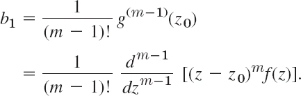
that converges for all points near z = z0 (except at z = z0 itself), in some domain of the form 0 < |z − z0| < R (sometimes called a deleted neighborhood, an old-fashioned term that we shall not use). Now comes the key idea. The coefficient b1 of the first negative power 1/(z − z0) of this Laurent series is given by the integral formula (2) in Sec. 16.1 with n = 1, namely,

Now, since we can obtain Laurent series by various methods, without using the integral formulas for the coefficients (see the examples in Sec. 16.1), we can find b1 by one of those methods and then use the formula for b1 for evaluating the integral, that is,
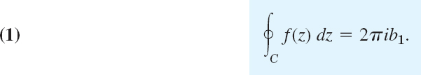
Here we integrate counterclockwise around a simple closed path C that contains z = z0 in its interior (but no other singular points of f(z) on or inside C!).
The coefficient b1 is called the residue of f(z) at and we denote it by

EXAMPLE 1 Evaluation of an Integral by Means of a Residue
Integrate the function f(z) = z−4 sin z counterclockwise around the unit circle C.
Solution. From (14) in Sec. 15.4 we obtain the Laurent series

which converges for |z| > 0 (that is, for all z ≠ 0). This series shows that f(z) has a pole of third order at z = 0 and the residue ![]() From (1) we thus obtain the answer
From (1) we thus obtain the answer

EXAMPLE 2 CAUTION! Use the Right Laurent Series!
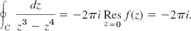
Integrate f(z) = 1/(z3 − z4) clockwise around the circle C: ![]()
Solution. z3 − z4 = z3(1 − z) shows that f(z) is singular at z = 0 and z = 1. Now z = 1 lies outside C. Hence it is of no interest here. So we need the residue of f(z) at 0. We find it from the Laurent series that converges for 0 < |z| < 1. This is series (I) in Example 4, Sec. 16.1,
![]()
We see from it that this residue is 1. Clockwise integration thus yields

we would have obtained the wrong answer, 0, because this series has no power 1/z.
Formulas for Residues
To calculate a residue at a pole, we need not produce a whole Laurent series, but, more economically, we can derive formulas for residues once and for all.
Simple Poles at z0. A first formula for the residue at a simple pole is

A second formula for the residue at a simple pole is
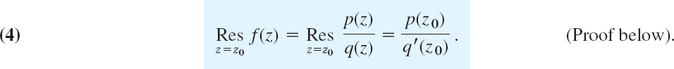
In (4) we assume that f(z) = p(z)/q(z) with p(z0) ≠ 0 and q(z) has a simple zero at z0, so that f(z) has a simple pole at z0 by Theorem 4 in Sec. 16.2.
PROOF
We prove (3). For a simple pole at z = z0 the Laurent series (1), Sec. 16.1,
![]()
Here b1 ≠ 0. (Why?) Multiplying both sides by z − z0 and then letting z → z0, we obtain the formula (3):
![]()
where the last equality follows from continuity (Theorem 1, Sec. 15.3).
We prove (4). The Taylor series of q(z) at a simple zero z0 is
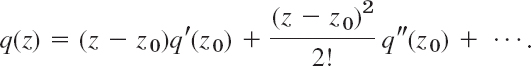
Substituting this into f = p/q and then f into (3) gives
![]()
z − z0 cancels. By continuity, the limit of the denominator is q′(z0) and (4) follows.
EXAMPLE 3 Residue at a Simple Pole
f(z) = (9z + i)/(z3 + z) has a simple pole at i because z2 + 1 = (z + i)(z − i), and (3) gives the residue
![]()
By (4) with p(i) = 9i + i and q′(z) = 3z2 + 1 we confirm the result,

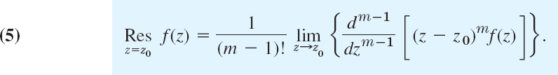
Poles of Any Order at z0. The residue of f(z) at an mth-order pole at z0 is
In particular, for a second-order pole (m = 2),

PROOF
We prove (5). The Laurent series of f(z) converging near z0 (except at z0 itself) is (Sec. 16.2)

where bm ≠ 0. The residue wanted is b1. Multiplying both sides by (z − z0)m gives
![]()
We see that b1 is now the coefficient of the power (z − z0)m−1 of the power series of g(z) = (z − z0)mf(z). Hence Taylor's theorem (Sec. 15.4) gives (5):
EXAMPLE 4 Residue at a Pole of Higher Order
f(z) = 50z/(z3 + 2z2 − 7z + 4) has a pole of second order at z = 1 because the denominator equals (z + 4)(z − 1)2 (verify!). From (5*) we obtain the residue

Several Singularities Inside the Contour. Residue Theorem
Residue integration can be extended from the case of a single singularity to the case of several singularities within the contour C. This is the purpose of the residue theorem. The extension is surprisingly simple.
Let f(z) be analytic inside a simple closed path C and on C, except for finitely many singular points z1, z2, …, zk inside C. Then the integral of f(z) taken counterclockwise around C equals 2πi times the sum of the residues of f(z) at z1, …, zk:

PROOF
We enclose each of the singular points zj in a circle Cj with radius small enough that those k circles and C are all separated (Fig. 373 where k = 3). Then f(z) is analytic in the multiply connected domain D bounded by C and C1, …, Ck and on the entire boundary of D. From Cauchy's integral theorem we thus have

the integral along C being taken counterclockwise and the other integrals clockwise (as in Figs. 354 and 355, Sec. 14.2). We take the integrals over C1, …, Ck to the right and compensate the resulting minus sign by reversing the sense of integration. Thus,

where all the integrals are now taken counterclockwise. By (1) and (2),

so that (8) gives (6) and the residue theorem is proved.

This important theorem has various applications in connection with complex and real integrals. Let us first consider some complex integrals. (Real integrals follow in the next section.)
EXAMPLE 5 Integration by the Residue Theorem. Several Contours
Evaluate the following integral counterclockwise around any simple closed path such that (a) 0 and 1 are inside C, (b) 0 is inside, 1 outside, (c) 1 is inside, 0 outside, (d) 0 and 1 are outside.
Solution. The integrand has simple poles at 0 and 1, with residues [by (3)]
![]()
[Confirm this by (4).] Answer: (a) 2πi(−4 + 1) = −6πi, (b) −8πi, (c) 2πi, (d) 0.
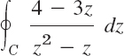
EXAMPLE 6 Another Application of the Residue Theorem
Integrate (tan z)/(z2 − 1) counterclockwise around the circle C: ![]() .
.
Solution. tan z is not analytic at ±π/2, ±3π/2, …, but all these points lie outside the contour C. Because of the denominator z2 − 1 = (z − 1)(z + 1) the given function has simple poles at ±1. We thus obtain from (4) and the residue theorem

EXAMPLE 7 Poles and Essential Singularities
Evaluate the following integral, where C is the ellipse 9x2 + y2 = 9 (counterclockwise, sketch it).

Solution. Since z4 − 16 = 0 at ±2i and ±2, the first term of the integrand has simple poles at ±2i inside C, with residues [by (4); note that e2πi = 1]

and simple poles at ±2, which lie outside C, so that they are of no interest here. The second term of the integrand has an essential singularity at 0, with residue π2/2 as obtained from

Answer: ![]() by the residue theorem.
by the residue theorem.
- Verify the calculations in Example 3 and find the other residues.
- Verify the calculations in Example 4 and find the other residue.
3–12 RESIDUES
Find all the singularities in the finite plane and the corresponding residues. Show the details.
- 3.

- 4.

- 5.

- 6. tan z
- 7. cot πz
- 8.

- 9.

- 10.

- 11.

- 12. e1/(1−z)
- 13. CAS PROJECT. Residue at a Pole. Write a program for calculating the residue at a pole of any order in the finite plane. Use it for solving Probs. 5–10.
14–25 RESIDUE INTEGRATION
Evaluate (counterclockwise). Show the details.
- 14.
 C: |z − 2 − i| = 3.2
 - 15.
 C: |z − 0.2| = 0.2
 - 16.
 the unit circle
 - 17.
 C: |z − πi/2| = 4.5
 - 18.
 C: |z − 1| = 2
 - 19.
 C: |z − 2i| = 2
 - 20.
 C: |z − i| = 3
 - 21.

- 22.
 C the unit circle
 - 23.
 C the unit circle
 - 24.
 C: |z| = 1.5
 - 25.
 |z| = π
16.4 Residue Integration of Real Integrals
Surprisingly, residue integration can also be used to evaluate certain classes of complicated real integrals. This shows an advantage of complex analysis over real analysis or calculus.
Integrals of Rational Functions of cos θ and sin θ
We first consider integrals of the type

where F(cos θ, sin θ) is a real rational function of cos θ and sin θ [for example, (sin2θ)/(5 − 4 cos θ)] and is finite (does not become infinite) on the interval of integration. Setting eiθ = z, we obtain
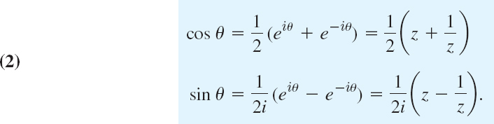
Since F is rational in cos θ and sin θ, Eq. (2) shows that F is now a rational function of z, say, f(z). Since dz/dθ = ieiθ, we have dθ = dz/iz and the given integral takes the form
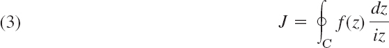
and, as θ ranges from 0 to 2π in (1), the variable z = eiθ ranges counterclockwise once around the unit circle |z| = 1. (Review Sec. 13.5 if necessary.)
EXAMPLE 1 An Integral of the Type (1)
Show by the present method that ![]()
Solution. We use cos θ = ![]() (z + 1/z) and dθ = dz/iz. Then the integral becomes
(z + 1/z) and dθ = dz/iz. Then the integral becomes

We see that the integrand has a simple pole at ![]() outside the unit circle C, so that it is of no interest here, and another simple pole at
outside the unit circle C, so that it is of no interest here, and another simple pole at ![]() (where
(where ![]() ) inside C with residue [by (3), Sec. 16.3]
) inside C with residue [by (3), Sec. 16.3]

Answer: ![]() (Here −2/i is the factor in front of the last integral.)
(Here −2/i is the factor in front of the last integral.)
As another large class, let us consider real integrals of the form
Such an integral, whose interval of integration is not finite is called an improper integral, and it has the meaning
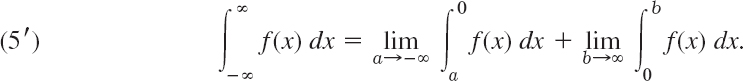
If both limits exist, we may couple the two independent passages to − ∞ and ∞, and write
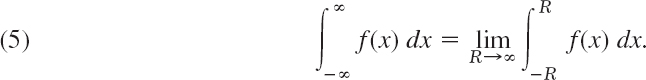
The limit in (5) is called the Cauchy principal value of the integral. It is written
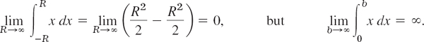
It may exist even if the limits in (5′) do not. Example:
We assume that the function f(x) in (4) is a real rational function whose denominator is different from zero for all real x and is of degree at least two units higher than the degree of the numerator. Then the limits in (5′) exist, and we may start from (5). We consider the corresponding contour integral

around a path C in Fig. 374. Since f(x) is rational, f(z) has finitely many poles in the upper half-plane, and if we choose R large enough, then C encloses all these poles. By the residue theorem we then obtain

where the sum consists of all the residues of f(z) at the points in the upper half-plane at which f(z) has a pole. From this we have

We prove that, if R → ∞, the value of the integral over the semicircle S approaches zero. If we set z = Reiθ, then S is represented by R = const, and as z ranges along S, the variable θ ranges from 0 to π. Since, by assumption, the degree of the denominator of f(z) is at least two units higher than the degree of the numerator, we have
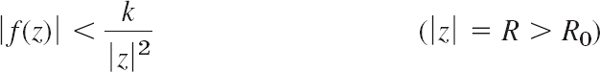

Fig. 374. Path C of the contour integral in (5*)
for sufficiently large constants k and R0. By the ML-inequality in Sec. 14.1,

Hence, as R approaches infinity, the value of the integral over S approaches zero, and (5) and (6) yield the result

where we sum over all the residues of f(z) at the poles of f(z) in the upper half-plane.
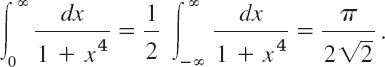
EXAMPLE 2 An Improper Integral from 0 to ∞
Using (7), show that
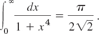

Fig. 375. Example 2
Solution. Indeed, f(z) = 1/(1 + z4) has four simple poles at the points (make a sketch)
![]()
The first two of these poles lie in the upper half-plane (Fig. 375). From (4) in the last section we find the residues

(Here we used eπi = −1 and e−2πi = 1.) By (1) in Sec. 13.6 and (7) in this section,
![]()
Since 1/(1 + x4) is an even function, we thus obtain, as asserted,
Fourier Integrals
The method of evaluating (4) by creating a closed contour (Fig. 374) and “blowing it up” extends to integrals

as they occur in connection with the Fourier integral (Sec. 11.7).
If f(x) is a rational function satisfying the assumption on the degree as for (4), we may consider the corresponding integral
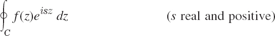
over the contour C in Fig. 374. Instead of (7) we now get

where we sum the residues of f(z)eisz at its poles in the upper half-plane. Equating the real and the imaginary parts on both sides of (9), we have

To establish (9), we must show [as for (4)] that the value of the integral over the semicircle S in Fig. 374 approaches 0 as R → ∞. Now s > 0 and S lies in the upper half-plane y ![]() 0. Hence
0. Hence
![]()
From this we obtain the inequality |f(z)eisz| = |f(z)||eisz| ![]() |f(z)| (s > 0, y
|f(z)| (s > 0, y ![]() 0). This reduces our present problem to that for (4). Continuing as before gives (9) and (10).
0). This reduces our present problem to that for (4). Continuing as before gives (9) and (10).
EXAMPLE 3 An Application of (10)
Show that

Solution. In fact, eisz/(k2 + z2) has only one pole in the upper half-plane, namely, a simple pole at z = ik, and from (4) in Sec. 16.3 we obtain

Thus

Since eisz = cos sx + i sin sx, this yields the above results [see also (15) in Sec. 11.7.]
Another Kind of Improper Integral
We consider an improper integral

whose integrand becomes infinite at a point a in the interval of integration,
![]()
By definition, this integral (11) means

where both ![]() and η approach zero independently and through positive values. It may happen that neither of these two limits exists if
and η approach zero independently and through positive values. It may happen that neither of these two limits exists if ![]() and η go to 0 independently, but the limit
and η go to 0 independently, but the limit
exists. This is called the Cauchy principal value of the integral. It is written

For example,
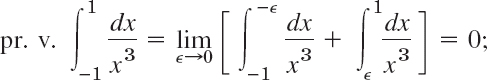
the principal value exists, although the integral itself has no meaning.
In the case of simple poles on the real axis we shall obtain a formula for the principal value of an integral from − ∞ to ∞. This formula will result from the following theorem.
THEOREM 1 Simple Poles on the Real Axis
If f(z) has a simple pole at z = a on the real axis, then (Fig. 376)
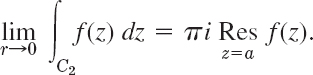

Fig. 376. Theorem 1
PROOF
By the definition of a simple pole (Sec. 16.2) the integrand f(z) has for 0 < |z − a| < R the Laurent series

Here g(z) is analytic on the semicircle of integration (Fig. 376)
![]()
and for all z between C2 and the x-axis, and thus bounded on C2, say, |g(z)| ![]() M. By integration,
M. By integration,

The second integral on the right cannot exceed Mπr in absolute value, by the ML-inequality (Sec. 14.1), and ML = Mπr → 0 as r → 0.
Figure 377 shows the idea of applying Theorem 1 to obtain the principal value of the integral of a rational function f(x) from − ∞ to ∞. For sufficiently large R the integral over the entire contour in Fig. 377 has the value J given by 2πi times the sum of the residues of f(z) at the singularities in the upper half-plane. We assume that f(x) satisfies the degree condition imposed in connection with (4). Then the value of the integral over the large semicircle S approaches 0 as R → ∞. For r → 0 the integral over C2 (clockwise!) approaches the value
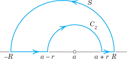
Fig. 377. Application of Theorem 1
by Theorem 1. Together this shows that the principal value P of the integral from −∞ to ∞ plus K equals J; hence P = J − K = J + πi Resz=a f(z). If f(z) has several simple poles on the real axis, then K will be −πi times the sum of the corresponding residues. Hence the desired formula is

where the first sum extends over all poles in the upper half-plane and the second over all poles on the real axis, the latter being simple by assumption.
EXAMPLE 4 Poles on the Real Axis
Find the principal value
Solution. Since
![]()
the integrand f(x), considered for complex z, has simple poles at

and at z = −i in the lower half-plane, which is of no interest here. From (14) we get the answer

More integrals of the kind considered in this section are included in the problem set. Try also your CAS, which may sometimes give you false results on complex integrals.
1–9 INTEGRALS INVOLVING COSINE AND SINE
Evaluate the following integrals and show the details of your work.
10–22 IMPROPER INTEGRALS: INFINITE INTERVAL OF INTEGRATION
Evaluate the following integrals and show details of your work.
- 10.

- 11.

- 12.

- 13.
- 14.

- 15.

- 16.

- 17.

- 18.

- 19.

- 20.

- 21.
- 22.

23–28 IMPROPER INTEGRALS: POLES ON THE REAL AXIS
Find the Cauchy principal value (showing details):
- 23.

- 24.
- 25.

- 26.

- 27. CAS EXPERIMENT. Simple Poles on the Real Axis. Experiment with integrals
 f(x) dx, f(x) = [(x − a1)(x − a2) … (x − ak)]−1, aj real and all different, k > 1. Conjecture that the principal value of these integrals is 0. Try to prove this for a special k, say, k = 3. For general k.
 - 28. TEAM PROJECT. Comments on Real Integrals.
(a) Formula (10) follows from (9). Give the details.
(b) Use of auxiliary results. Integrating e−z2 around the boundary C of the rectangle with vertices −a, a, a + ib, −a + ib, letting a − ∞, and using

show that

(This integral is needed in heat conduction in Sec. 12.7.)
(c) Inspection. Solve Probs. 13 and 17 without calculation.
CHAPTER 16 REVIEW QUESTIONS AND PROBLEMS
- What is a Laurent series? Its principal part? Its use? Give simple examples.
- What kind of singularities did we discuss? Give definitions and examples.
- What is the residue? Its role in integration? Explain methods to obtain it.
- Can the residue at a singularity be zero? At a simple pole? Give reason.
- State the residue theorem and the idea of its proof from memory.
- How did we evaluate real integrals by residue integration? How did we obtain the closed paths needed?
- What are improper integrals? Their principal value? Why did they occur in this chapter?
- What do you know about zeros of analytic functions? Give examples.
- What is the extended complex plane? The Riemann sphere R? Sketch z = 1 + i on R.
- What is an entire function? Can it be analytic at infinity? Explain the definitions.
11–18 COMPLEX INTEGRALS
Integrate counterclockwise around C. Show the details.
- 11.
 C: |z| = π
 - 12. e2/z, C: |z − 1 − i| = 2
- 13.
 C: |z| = 3
 - 14. C: |z − i| = πi/2
- 15.
 C: |z − 5| = 1
 - 16.
 C: |z| = 4
 - 17.
 n = 0, 1, 2, …, C: |z| = 1
 - 18. cot 4z,

19–25 REAL INTEGRALS
Evaluate by the methods of this chapter. Show details.
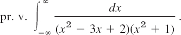
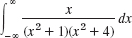
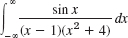
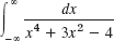
- 19.

- 20.

- 21.
- 22.

- 23.

- 24.

- 25.

SUMMARY OF CHAPTER 16 Laurent Series. Residue Integration
A Laurent series is a series of the form

or, more briefly written [but this means the same as (1)!]

where n = 0, ±1, ±2, …. This series converges in an open annulus (ring) A with center z0. In A the function f(z) is analytic. At points not in A it may have singularities. The first series in (1) is a power series. In a given annulus, a Laurent series of f(z) is unique, but f(z) may have different Laurent series in different annuli with the same center.
Of particular importance is the Laurent series (1) that converges in a neighborhood of z0 except at z0 itself, say, for 0 < |z − z0| < R (R > 0, suitable). The series (or finite sum) of the negative powers in this Laurent series is called the principal part of f(z) at z0. The coefficient b1 of 1/(z − z0) in this series is called the residue of f(z) at z0 and is given by [see (1) and (1*)]

b1 can be used for integration as shown in (2) because it can be found from

provided f(z) has at z0 a pole of orderm; by definition this means that principal part has 1/(z − z0)m as its highest negative power. Thus for a simple pole (m = 1),

If the principal part is an infinite series, the singularity of f(z) at z0 is called an essential singularity (Sec. 16.2).
Section 16.2 also discusses the extended complex plane, that is, the complex plane with an improper point ∞ (“infinity”) attached.
Residue integration may also be used to evaluate certain classes of complicated real integrals (Sec. 16.4).