
14
Complex Integration

Chapter 13 laid the groundwork for the study of complex analysis, covered complex numbers in the complex plane, limits, and differentiation, and introduced the most important concept of analyticity. A complex function is analytic in some domain if it is differentiable in that domain. Complex analysis deals with such functions and their applications. The Cauchy–Riemann equations, in Sec. 13.4, were the heart of Chapter 13 and allowed a means of checking whether a function is indeed analytic. In that section, we also saw that analytic functions satisfy Laplace's equation, the most important PDE in physics.
We now consider the next part of complex calculus, that is, we shall discuss the first approach to complex integration. It centers around the very important Cauchy integral theorem (also called the Cauchy–Goursat theorem) in Sec. 14.2. This theorem is important because it allows, through its implied Cauchy integral formula of Sec. 14.3, the evaluation of integrals having an analytic integrand. Furthermore, the Cauchy integral formula shows the surprising result that analytic functions have derivatives of all orders. Hence, in this respect, complex analytic functions behave much more simply than real-valued functions of real variables, which may have derivatives only up to a certain order.
Complex integration is attractive for several reasons. Some basic properties of analytic functions are difficult to prove by other methods. This includes the existence of derivatives of all orders just discussed. A main practical reason for the importance of integration in the complex plane is that such integration can evaluate certain real integrals that appear in applications and that are not accessible by real integral calculus.
Finally, complex integration is used in connection with special functions, such as gamma functions (consult [GenRef1]), the error function, and various polynomials (see [GenRef10]). These functions are applied to problems in physics.
The second approach to complex integration is integration by residues, which we shall cover in Chapter 16.
Prerequisite: Chap. 13.
Section that may be omitted in a shorter course: 14.1, 14.5.
References and Answers to Problems: App. 1 Part D, App. 2.
14.1 Line Integral in the Complex Plane
As in calculus, in complex analysis we distinguish between definite integrals and indefinite integrals or antiderivatives. Here an indefinite integral is a function whose derivative equals a given analytic function in a region. By inverting known differentiation formulas we may find many types of indefinite integrals.
Complex definite integrals are called (complex) line integrals. They are written

Here the integrand f(z) is integrated over a given curve C or a portion of it (an arc, but we shall say “curve” in either case, for simplicity). This curve C in the complex plane is called the path of integration. We may represent C by a parametric representation

The sense of increasing t is called the positive sense on C, and we say that C is oriented by (1).
For instance, z(t) = t + 3it (0 ![]() t
t ![]() 2) gives a portion (a segment) of the line y = 3x. The function z(t) = 4 cos t + 4i sin t(−π
2) gives a portion (a segment) of the line y = 3x. The function z(t) = 4 cos t + 4i sin t(−π ![]() t
t ![]() π) represents the circle |z| = 4, and so on. More examples follow below.
π) represents the circle |z| = 4, and so on. More examples follow below.
We assume C to be a smooth curve, that is, C has a continuous and nonzero derivative

at each point. Geometrically this means that C has everywhere a continuously turning tangent, as follows directly from the definition

Here we use a dot since a prime ′ denotes the derivative with respect to z.
Definition of the Complex Line Integral
This is similar to the method in calculus. Let C be a smooth curve in the complex plane given by (1), and let f(z) be a continuous function given (at least) at each point of C. We now subdivide (we “partition”) the interval a ![]() t
t ![]() b in (1) by points
b in (1) by points
![]()
where t0 < t1 < … < tn. To this subdivision there corresponds a subdivision of C by points
![]()

Fig. 339. Tangent vector ![]() of a curve C in the complex plane given by z(t). The arrowhead on the curve indicates the positive sense (sense of increasing t)
of a curve C in the complex plane given by z(t). The arrowhead on the curve indicates the positive sense (sense of increasing t)

Fig. 340. Complex line integral
where zj = z(tj). On each portion of subdivision of C we choose an arbitrary point, say, a point ζ1 between z0 and z1 (that is, ζ1 = z(t) where t satisfies t0 ![]() t
t ![]() t1), a point ζ2 between z1 and z2, etc. Then we form the sum
t1), a point ζ2 between z1 and z2, etc. Then we form the sum

We do this for each n = 2, 3, … in a completely independent manner, but so that the greatest |Δtm| = |tm − tm−1| approaches zero as n → ∞. This implies that the greatest |Δzm| also approaches zero. Indeed, it cannot exceed the length of the arc of C from zm−1 to zm and the latter goes to zero since the arc length of the smooth curve C is a continuous function of t. The limit of the sequence of complex numbers S2, S3, … thus obtained is called the line integral (or simply the integral) of f(z) over the path of integration C with the orientation given by (1). This line integral is denoted by

if C is a closed path (one whose terminal point Z coincides with its initial point z0, as for a circle or for a curve shaped like an 8).
General Assumption. All paths of integration for complex line integrals are assumed to be piecewise smooth, that is, they consist of finitely many smooth curves joined end to end.
Basic Properties Directly Implied by the Definition
- Linearity. Integration is a linear operation, that is, we can integrate sums term by term and can take out constant factors from under the integral sign. This means that if the integrals of f1 and f2 over a path C exist, so does the integral of k1f1 + k2f2 over the same path and

- Sense reversal in integrating over the same path, from to Z0 to Z (left) and from Z to (right), introduces a minus sign as shown,

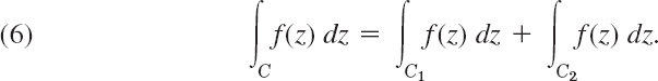
- Partitioning of path (see Fig. 341)

Existence of the Complex Line Integral
Our assumptions that f(z) is continuous and C is piecewise smooth imply the existence of the line integral (3). This can be seen as follows.
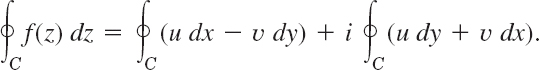
As in the preceding chapter let us write f(z) = u(x, y) + iv(x, y). We also set
![]()
Then (2) may be written
![]()
where u = u(ζm, ηm), v = v(ζm, ηm) and we sum over m from 1 to n. Performing the multiplication, we may now split up Sn into four sums:
![]()
These sums are real. Since f is continuous, u and v are continuous. Hence, if we let n approach infinity in the aforementioned way, then the greatest Δxm and Δym will approach zero and each sum on the right becomes a real line integral:

This shows that under our assumptions on f and C the line integral (3) exists and its value is independent of the choice of subdivisions and intermediate points ζm.
First Evaluation Method: Indefinite Integration and Substitution of Limits
This method is the analog of the evaluation of definite integrals in calculus by the well-known formula where

where [F′(x) = f(x)].
It is simpler than the next method, but it is suitable for analytic functions only. To formulate it, we need the following concept of general interest.
A domain D is called simply connected if every simple closed curve (closed curve without self-intersections) encloses only points of D.
For instance, a circular disk is simply connected, whereas an annulus (Sec. 13.3) is not simply connected. (Explain!)
THEOREM 1 Indefinite Integration of Analytic Functions
Let f(z) be analytic in a simply connected domain D. Then there exists an indefinite integral of f(z) in the domain D, that is, an analytic function F(z) such that F′(z) = f(z) in D, and for all paths in D joining two points z0 and z1 in D we have
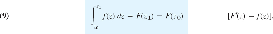
(Note that we can write z0 and z1 instead of C, since we get the same value for all those C from z0 to z1.)
This theorem will be proved in the next section.
Simple connectedness is quite essential in Theorem 1, as we shall see in Example 5.
Since analytic functions are our main concern, and since differentiation formulas will often help in finding F(z) for a given f(z) = F′(z), the present method is of great practical interest.
If f(z) is entire (Sec. 13.5), we can take for D the complex plane (which is certainly simply connected).


![]() Here D is the complex plane without 0 and the negative real axis (where Ln z is not analytic). Obviously, D is a simply connected domain.
Here D is the complex plane without 0 and the negative real axis (where Ln z is not analytic). Obviously, D is a simply connected domain.
Second Evaluation Method: Use of a Representation of a Path
This method is not restricted to analytic functions but applies to any continuous complex function.
THEOREM 2 Integration by the Use of the Path
Let C be a piecewise smooth path, represented by z = z(t), where a ![]() t
t ![]() b. Let f(z) be a continuous function on C. Then
b. Let f(z) be a continuous function on C. Then

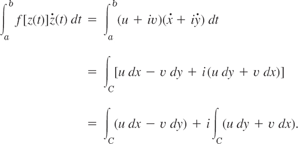
The left side of (10) is given by (8) in terms of real line integrals, and we show that the right side of (10) also equals (8). We have z = x + iy, hence ![]() We simply write u for u[x(t), y(t)] and v for v[x(t), y(t)]. We also have
We simply write u for u[x(t), y(t)] and v for v[x(t), y(t)]. We also have ![]() and
and ![]() Consequently, in (10)
Consequently, in (10)
COMMENT. In (7) and (8) of the existence proof of the complex line integral we referred to real line integrals. If one wants to avoid this, one can take (10) as a definition of the complex line integral.
Steps in Applying Theorem 2
- Represent the path C in the form z(t)(a
 t b).
t b). - Calculate the derivative

- Substitute z(t) for every z in f(z) (hence x(t) for x and y(t) for y).
- Integrate
 over t from a to b.
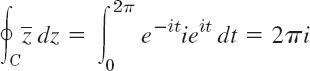
EXAMPLE 5 A Basic Result: Integral of 1/zAround the Unit Circle
We show that by integrating 1/z counterclockwise around the unit circle (the circle of radius 1 and center 0; see Sec. 13.3) we obtain

This is a very important result that we shall need quite often.
Solution. (A) We may represent the unit circle C in Fig. 330 of Sec. 13.3 by
![]()
so that counterclockwise integration corresponds to an increase of t from 0 to 2π.
- (B) Differentiation gives
 (chain rule!).
 - (C) By substitution, f(z(t)) = 1/z(t) = e−it.
- (D) From (10) we thus obtain the result

Check this result by using z(t) = cos t + i sin t.
Simple connectedness is essential in Theorem 1. Equation (9) in Theorem 1 gives 0 for any closed path because then z1 = z0, so that F(z1) − F(z0) = 0. Now 1/z is not analytic at z = 0. But any simply connected domain containing the unit circle must contain z = 0, so that Theorem 1 does not apply—it is not enough that 1/z is analytic in an annulus, say, ![]() because an annulus is not simply connected!
because an annulus is not simply connected!
EXAMPLE 6 Integral of 1/zm with Integer Power m
Let f(z) = (z − z0)m where m is the integer and z0 a constant. Integrate counterclockwise around the circle C of radius ρ with center at z0 (Fig. 342).

Fig. 342. Path in Example 6
Solution. We may represent C in the form
![]()
Then we have
![]()
and obtain

By the Euler formula (5) in Sec. 13.6 the right side equals

If m = −1, we have ρm + 1 = 1, cos 0 = 1, sin 0 = 0. We thus obtain 2πi. For integer m ≠ −1 each of the two integrals is zero because we integrate over an interval of length 2π, equal to a period of sine and cosine. Hence the result is

Dependence on path. Now comes a very important fact. If we integrate a given function f(z) from a point z0 to a point z1 along different paths, the integrals will in general have different values. In other words, a complex line integral depends not only on the endpoints of the path but in general also on the path itself. The next example gives a first impression of this, and a systematic discussion follows in the next section.
EXAMPLE 7 Integral of a Nonanalytic Function. Dependence on Path
Integrate f(z) = Re z = x from 0 to 1 + 2i (a) along C* in Fig. 343, (b) along C consisting of C1 and C2
Solution. (a) C* can be represented by z(t) = t + 2it (0 ![]() t
t ![]() 1). Hence
1). Hence ![]() and f[z(t)] = x(t) = t on C*. We now calculate
and f[z(t)] = x(t) = t on C*. We now calculate


Fig. 343. Paths in Example 7
(b) We now have

Using (6) we calculate

Note that this result differs from the result in (a).
Bounds for Integrals. ML-Inequality
There will be a frequent need for estimating the absolute value of complex line integrals. The basic formula is

L is the length of C and M a constant such that |f(z)| ![]() M everywhere on C.
M everywhere on C.
PROOF
Taking the absolute value in (2) and applying the generalized inequality (6*) in Sec. 13.2, we obtain

Now |Δzm| is the length of the chord whose endpoints are zm−1 and zm (see Fig. 340). Hence the sum on the right represents the length L* of the broken line of chords whose endpoints are z0, z1, …, zn(= Z). If n approaches infinity in such a way that the greatest |Δtm| and thus |Δzm| approach zero, then L* approaches the length L of the curve C, by the definition of the length of a curve. From this the inequality (13) follows.
We cannot see from (13) how close to the bound ML the actual absolute value of the integral is, but this will be no handicap in applying (13). For the time being we explain the practical use of (13) by a simple example.
EXAMPLE 8 Estimation of an Integral
Find an upper bound for the absolute value of the integral
![]()
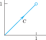
Fig. 344. Path in Example 8
Solution. ![]() and |f(z)| = |z2 |
and |f(z)| = |z2 | ![]() 2 on C gives by (13)
2 on C gives by (13)

The absolute value of the integral is ![]() (see Example 1).
(see Example 1).
Summary on Integration. Line integrals of f(z) can always be evaluated by (10), using a representation (1) of the path of integration. If f(z) is analytic, indefinite integration by (9) as in calculus will be simpler (proof in the next section).
1–10 FIND THE PATH and sketch it.

- z(t) = 3 + i + (1 − i)t (0 t 3)
- z(t) = t + 2it2 (1 t 2)
- z(t) = t + (1 − t)2i (−1 t 1)

- z(t) = 1 + i + e−πit (0 t 2)
- z(t) = 2 + 4eπit/2 (0 t 2)
- z(t) = 5e−it (0 t π/2)
- z(t) = t + it3 (−2 t 2)
- z(t) = 2 cos t + i sin t (0 t 2π)
11–20 FIND A PARAMETRIC REPRESENTATION
and sketch the path.
- 11. Segment from (−1, 1) to (1, 3)
- 12. From (0, 0) to (2, 1) along the axes
- 13. Upper half of |z − 2 + i| = 2 from (4, −1) to (0, −1)
- 14. Unit circle, clockwise
- 15. x2 − 4y2 = 4, the branch through (2, 0)
- 16. Ellipse 4x2 + 9y2 = 36, counterclockwise
- 17. |z + a + ib| = r, clockwise
- 18. y = 1/x from (1, 1) to

- 19. Parabola

- 20. 4(x − 2)2 + 5(y + 1)2 = 20
21–30 INTEGRATION
Integrate by the first method or state why it does not apply and use the second method. Show the details.
- 21. ∫C Re z dz, C the shortest path from 1 + i to 3 + 3i
- 22. ∫C Re z dz, C the parabola
 from 1 + i to 3 + 3i
 - 23. ∫C ez dz, C the shortest path from πi to 2πi
- 24. ∫C cos 2z dz, C the semicircle |z| = π, x
 0 from −πi to πi
 - 25. ∫C z exp (z2) dz, C from 1 along the axes to i
- 26. ∫C (z + z−1)dz, C the unit circle, counterclockwise
- 27. ∫C sec2z dz, any path from π/4 to πi/4
- 28.
 C the circle |z − 2i| = 4, clockwise
 - 29. ∫C Im z2dz counterclockwise around the triangle with vertices 0, 1, i
- 30. ∫C Re z2dz clockwise around the boundary of the square with vertices 0, i, 1 + i, 1
- 31. CAS PROJECT. Integration. Write programs for the two integration methods. Apply them to problems of your choice. Could you make them into a joint program that also decides which of the two methods to use in a given case?
- 32. Sense reversal. Verify (5) for f(z) = z2, where C is the segment from −1 − i to 1 + i.
- 33. Path partitioning. Verify (6) for f(z) = 1/z and C1 and C2 the upper and lower halves of the unit circle.
- 34. TEAM EXPERIMENT. Integration. (a) Comparison. First write a short report comparing the essential points of the two integration methods.
- (b) Comparison. Evaluate ∫C f(z)dz by Theorem 1 and check the result by Theorem 2, where:
- f(z) = z4 and C is the semicircle |z| = 2 from −2i to 2i in the right half-plane,
- f(z) = e2z and C is the shortest path from 0 to 1 + 2i.
- (c) Continuous deformation of path. Experiment with a family of paths with common endpoints, say, z(t) = t + ia sin t, 0 t π, with real parameter a. Integrate nonanalytic functions (Re z, Re(z2), etc.) and explore how the result depends on a. Then take analytic functions of your choice. (Show the details of your work.) Compare and comment.
- (d) Continuous deformation of path. Choose another family, for example, semi-ellipses z(t) = a cos t + i sin t, −π/2 t π/2, and experiment as in (c).
- (b) Comparison. Evaluate ∫C f(z)dz by Theorem 1 and check the result by Theorem 2, where:
- 35. ML-inequality. Find an upper bound of the absolute value of the integral in Prob. 21.
14.2 Cauchy's Integral Theorem
This section is the focal point of the chapter. We have just seen in Sec. 14.1 that a line integral of a function f(z) generally depends not merely on the endpoints of the path, but also on the choice of the path itself. This dependence often complicates situations. Hence conditions under which this does not occur are of considerable importance. Namely, if f(z) is analytic in a domain D and D is simply connected (see Sec. 14.1 and also below), then the integral will not depend on the choice of a path between given points. This result (Theorem 2) follows from Cauchy's integral theorem, along with other basic consequences that make Cauchy's integral theorem the most important theorem in this chapter and fundamental throughout complex analysis.
Let us continue our discussion of simple connectedness which we started in Sec. 14.1.
- A simple closed path is a closed path (defined in Sec. 14.1) that does not intersect or touch itself as shown in Fig. 345. For example, a circle is simple, but a curve shaped like an 8 is not simple.

- A simply connected domain D in the complex plane is a domain (Sec. 13.3) such that every simple closed path in D encloses only points of D. Examples: The interior of a circle (“open disk”), ellipse, or any simple closed curve. A domain that is not simply connected is called multiply connected. Examples: An annulus (Sec. 13.3), a disk without the center, for example, 0 < |z| < 1. See also Fig. 346.
More precisely, a bounded domain D (that is, a domain that lies entirely in some circle about the origin) is called p-fold connected if its boundary consists of p closed connected sets without common points. These sets can be curves, segments, or single points (such as z = 0 for 0 < |z| < 1, for which p = 2). Thus, D has p − 1 “holes,” where “hole” may also mean a segment or even a single point. Hence an annulus is doubly connected (p = 2).

Fig. 346. Simply and multiply connected domains
THEOREM 1 Cauchy's Integral Theorem
If f(z) is analytic in a simply connected domain D, then for every simple closed path C in D,


Fig. 347. Cauchy's integral theorem
Before we prove the theorem, let us consider some examples in order to really understand what is going on. A simple closed path is sometimes called a contour and an integral over such a path a contour integral. Thus, (1) and our examples involve contour integrals.

for any closed path, since these functions are entire (analytic for all z).
EXAMPLE 2 Points Outside the Contour Where f(x) is Not Analytic

where C is the unit circle, sec z = 1/cos z is not analytic at z = ±π/2, ±3π/2, …, but all these points lie outside C; none lies on C or inside C. Similarly for the second integral, whose integrand is not analytic at z = ±2i outside C.
EXAMPLE 3 Nonanalytic Function
where C: z(t) = eit is the unit circle. This does not contradict Cauchy's theorem because ![]() is not analytic.
is not analytic.
EXAMPLE 4 Analyticity Sufficient, Not Necessary

where C is the unit circle. This result does not follow from Cauchy's theorem, because f(z) = 1/z2 is not analytic at z = 0. Hence the condition that f be analytic in D is sufficient rather than necessary for (1) to be true.
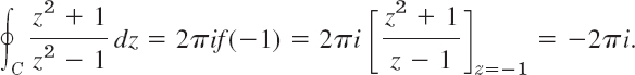
EXAMPLE 5 Simple Connectedness Essential

for counterclockwise integration around the unit circle (see Sec. 14.1). C lies in the annulus ![]() where 1/z is analytic, but this domain is not simply connected, so that Cauchy's theorem cannot be applied. Hence the condition that the domain D be simply connected is essential.
where 1/z is analytic, but this domain is not simply connected, so that Cauchy's theorem cannot be applied. Hence the condition that the domain D be simply connected is essential.
In other words, by Cauchy's theorem, if f(z) is analytic on a simple closed path C and everywhere inside C, with no exception, not even a single point, then (1) holds. The point that causes trouble here is z = 0 where 1/z is not analytic.
PROOF
Cauchy proved his integral theorem under the additional assumption that the derivative f′(z) is continuous (which is true, but would need an extra proof). His proof proceeds as follows. From (8) in Sec. 14.1 we have
Since f(z) is analytic in D, its derivative f′(z) exists in D. Since f′(z) is assumed to be continuous, (4) and (5) in Sec. 13.4 imply that u and v have continuous partial derivatives in D. Hence Green's theorem (Sec. 10.4) (with u and −v instead of F1 and F2) is applicable and gives

where R is the region bounded by C. The second Cauchy–Riemann equation (Sec. 13.4) shows that the integrand on the right is identically zero. Hence the integral on the left is zero. In the same fashion it follows by the use of the first Cauchy–Riemann equation that the last integral in the above formula is zero. This completes Cauchy's proof.
Goursat's proof without the condition that f′(z) is continuous1 is much more complicated. We leave it optional and include it in App. 4.
Independence of Path
We know from the preceding section that the value of a line integral of a given function f(z) from a point z1 to a point z2 will in general depend on the path C over which we integrate, not merely on z1 and z2. It is important to characterize situations in which this difficulty of path dependence does not occur. This task suggests the following concept. We call an integral of f(z) independent of path in a domainD if for every z1, z2 in D its value depends (besides on, f(z), of course) only on the initial point z1 and the terminal point z2, but not on the choice of the path C in D [so that every path in D from z1 to z2 gives the same value of the integral of f(z)].
THEOREM 2 Independence of Path
If f(z) is analytic in a simply connected domain D, then the integral of f(z) is independent of path in D.
PROOF
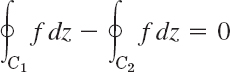
Let z1 and z2 be any points in D. Consider two paths C1 and C2 in D from z1 to z2 without further common points, as in Fig. 348. Denote by ![]() the path C2 with the orientation reversed (Fig. 349). Integrate from z1 over C1 to z2 and over
the path C2 with the orientation reversed (Fig. 349). Integrate from z1 over C1 to z2 and over ![]() back to z1. This is a simple closed path, and Cauchy's theorem applies under our assumptions of the present theorem and gives zero:
back to z1. This is a simple closed path, and Cauchy's theorem applies under our assumptions of the present theorem and gives zero:

But the minus sign on the right disappears if we integrate in the reverse direction, from z1 to z2, which shows that the integrals of f(z) over C1 and C2 are equal,

This proves the theorem for paths that have only the endpoints in common. For paths that have finitely many further common points, apply the present argument to each “loop” (portions of C1 and C2 between consecutive common points; four loops in Fig. 350). For paths with infinitely many common points we would need additional argumentation not to be presented here.
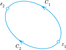


Fig. 350. Paths with more common points
Principle of Deformation of Path
This idea is related to path independence. We may imagine that the path C2 in (2) was obtained from C1 by continuously moving C1 (with ends fixed!) until it coincides with C2. Figure 351 shows two of the infinitely many intermediate paths for which the integral always retains its value (because of Theorem 2). Hence we may impose a continuous deformation of the path of an integral, keeping the ends fixed. As long as our deforming path always contains only points at which f(z) is analytic, the integral retains the same value. This is called the principle of deformation of path.

Fig. 351. Continuous deformation of path
EXAMPLE 6 A Basic Result: Integral of Integer Powers
From Example 6 in Sec. 14.1 and the principle of deformation of path it follows that

for counterclockwise integration around any simple closed path containing z0 in its interior.
Indeed, the circle |z − z0| = ρ in Example 6 of Sec. 14.1 can be continuously deformed in two steps into a path as just indicated, namely, by first deforming, say, one semicircle and then the other one. (Make a sketch).
Existence of Indefinite Integral
We shall now justify our indefinite integration method in the preceding section [formula (9) in Sec. 14.1]. The proof will need Cauchy's integral theorem.
THEOREM 3 Existence of Indefinite Integral
If f(z) is analytic in a simply connected domain D, then there exists an indefinite integral F(z) of f(z) in D—thus, F′(z) = f(z)—which is analytic in D, and for all paths in D joining any two points z0 and z1 in D, the integral of f(z) from z0 to z1 can be evaluated by formula (9) in Sec. 14.1.
PROOF
The conditions of Cauchy's integral theorem are satisfied. Hence the line integral of f(z) from any z0 in D to any z in D is independent of path in D. We keep z0 fixed. Then this integral becomes a function of z, call if F(z),

which is uniquely determined. We show that this F(z) is analytic in D and F′(z) = f(z). The idea of doing this is as follows. Using (4) we form the difference quotient

We now subtract f(z) from (5) and show that the resulting expression approaches zero as Δz → 0. The details are as follows.
We keep z fixed. Then we choose z + Δz in D so that the whole segment with endpoints z and z + Δz is in D (Fig. 352). This can be done because D is a domain, hence it contains a neighborhood of z. We use this segment as the path of integration in (5). Now we subtract f(z). This is a constant because z is kept fixed. Hence we can write

By this trick and from (5) we get a single integral:

Since f(z) is analytic, it is continuous (see Team Project (24d) in Sec. 13.3). An ![]() > 0 being given, we can thus find a δ > 0 such that |f(z*) − f(z)| <
> 0 being given, we can thus find a δ > 0 such that |f(z*) − f(z)| < ![]() when |z* − z| < δ. Hence, letting |Δz| < δ, we see that the ML-inequality (Sec. 14.1) yields
when |z* − z| < δ. Hence, letting |Δz| < δ, we see that the ML-inequality (Sec. 14.1) yields

By the definition of limit and derivative, this proves that

Since z is any point in D, this implies that F(z) is analytic in D and is an indefinite integral or antiderivative of f(z) in D, written


Also, if G′(z) = f(z), then F′(z) − G′(z) ≡ 0 in D; hence F(z) − G(z) is constant in D (see Team Project 30 in Problem Set 13.4). That is, two indefinite integrals of f(z) can differ only by a constant. The latter drops out in (9) of Sec. 14.1, so that we can use any indefinite integral of f(z). This proves Theorem 3.
Cauchy's Integral Theorem for Multiply Connected Domains
Cauchy's theorem applies to multiply connected domains. We first explain this for a doubly connected domain D with outer boundary curve C1 and inner C2 (Fig. 353). If a function f(z) is analytic in any domain D* that contains D and its boundary curves, we claim that

both integrals being taken counterclockwise (or both clockwise, and regardless of whether or not the full interior of C2 belongs to D*).

PROOF
By two cuts ![]() and
and ![]() (Fig. 354) we cut D into two simply connected domains D1 and D2 in which and on whose boundaries f(z) is analytic. By Cauchy's integral theorem the integral over the entire boundary of D1 (taken in the sense of the arrows in Fig. 354) is zero, and so is the integral over the boundary of D2, and thus their sum. In this sum the integrals over the cuts
(Fig. 354) we cut D into two simply connected domains D1 and D2 in which and on whose boundaries f(z) is analytic. By Cauchy's integral theorem the integral over the entire boundary of D1 (taken in the sense of the arrows in Fig. 354) is zero, and so is the integral over the boundary of D2, and thus their sum. In this sum the integrals over the cuts ![]() and
and ![]() cancel because we integrate over them in both directions—this is the key—and we are left with the integrals over C1 (counterclockwise) and C2 (clockwise; see Fig. 354); hence by reversing the integration over C2 (to counterclockwise) we have
cancel because we integrate over them in both directions—this is the key—and we are left with the integrals over C1 (counterclockwise) and C2 (clockwise; see Fig. 354); hence by reversing the integration over C2 (to counterclockwise) we have
and (6) follows.
For domains of higher connectivity the idea remains the same. Thus, for a triply connected domain we use three cuts ![]() (Fig. 355). Adding integrals as before, the integrals over the cuts cancel and the sum of the integrals over C1 (counterclockwise) and C2, C2 (clockwise) is zero. Hence the integral over C1 equals the sum of the integrals over C2 and C3 all three now taken counterclockwise. Similarly for quadruply connected domains, and so on.
(Fig. 355). Adding integrals as before, the integrals over the cuts cancel and the sum of the integrals over C1 (counterclockwise) and C2, C2 (clockwise) is zero. Hence the integral over C1 equals the sum of the integrals over C2 and C3 all three now taken counterclockwise. Similarly for quadruply connected domains, and so on.

Fig. 354. Doubly connected domain

Fig. 355. Triply connected domain
1–8 COMMENTS ON TEXT AND EXAMPLES
- Cauchy's Integral Theorem. Verify Theorem 1 for the integral of z2 over the boundary of the square with vertices ±1 ± i. Hint. Use deformation.
- For what contours C will it follow from Theorem 1 that
- Deformation principle. Can we conclude from Example 4 that the integral is also zero over the contour in Prob. 1?
- If the integral of a function over the unit circle equals 2 and over the circle of radius 3 equals 6, can the function be analytic everywhere in the annulus 1 < |z| < 3?
- Connectedness. What is the connectedness of the domain in which (cos z2)/(z4 + 1) is analytic?
- Path independence. Verify Theorem 2 for the integral of ez from 0 to 1 + i (a) over the shortest path and (b) over the x-axis to 1 and then straight up to 1 + i
- Deformation. Can we conclude in Example 2 that the integral of 1/(z2 + 4) over (a) |z − 2| and (b) |z − 2| = 3 is zero?
- TEAM EXPERIMENT. Cauchy's Integral Theorem.
(a) Main Aspects. Each of the problems in Examples 1–5 explains a basic fact in connection with Cauchy's theorem. Find five examples of your own, more complicated ones if possible, each illustrating one of those facts.
(b) Partial fractions. Write f(z) in terms of partial fractions and integrate it counterclockwise over the unit circle, where
- (i)

- (ii)

(c) Deformation of path. Review (c) and (d) of Team Project 34, Sec. 14.1, in the light of the principle of deformation of path. Then consider another family of paths with common endpoints, say, z(t) = t + ia (t − t2), 0
t 1, a a real constant, and experiment with the integration of analytic and nonanalytic functions of your choice over these paths (e.g., z, Im z, z2, Re z2, Im z2, etc.). - (i)
9–19 CAUCHY'S THEOREM APPLICABLE?
Integrate f(z) counterclockwise around the unit circle. Indicate whether Cauchy's integral theorem applies. Show the details.
- 9. f(z) = exp(−z2)
- 10.

- 11. f(z) = 1/(2z − 1)
- 12. f(z) =
 3
3 - 13. f(z) = 1/(z4 − 1.1)
- 14. f(z) = 1/
- 15. f(z) = Im z
- 16. f(z) = 1/(πz − 1)
- 17. f(z) = 1/|z|2
- 18. f(z) = 1/(4z − 3)
- 19. f(z) = z3 cot z
20–30 FURTHER CONTOUR INTEGRALS
Evaluate the integral. Does Cauchy's theorem apply? Show details.
- 20.
 C the boundary of the parallelogram with vertices ±i, ±(1 + i)
 - 21.
 C the circle |z| = π counterclockwise.
 - 22.

- 23.
 Use partial fractions.
 - 24.
 Use partial fractions.
 - 25.
 C consists of |z| = 2 counterclockwise and |z| = 1 clockwise.
 - 26.
 C the circle
  clockwise.
 - 27.
 C consists of |z| = 1 counterclockwise and |z| = 3 clockwise.
 - 28.
 C the boundary of the square with vertices ±1, ±i clockwise.
 - 29.
 C: |z − 4 − 2i| = 5.5 clockwise.
 - 30.
 C: |z − 2| = 4 clockwise. Use partial fractions.
14.3 Cauchy's Integral Formula
Cauchy's integral theorem leads to Cauchy's integral formula. This formula is useful for evaluating integrals as shown in this section. It has other important roles, such as in proving the surprising fact that analytic functions have derivatives of all orders, as shown in the next section, and in showing that all analytic functions have a Taylor series representation (to be seen in Sec. 15.4).
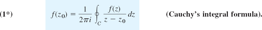
THEOREM 1 Cauchy's Integral Formula
Let f(z) be analytic in a simply connected domain D. Then for any point z0 in D and any simple closed path C in D that encloses z0 (Fig. 356),

the integration being taken counterclockwise. Alternatively (for representing f(z) by a contour integral, divide (1) by 2πi),
PROOF
By addition and subtraction, f(z) = f(z0) + [f(z) − f(z0)]. Inserting this into (1) on the left and taking the constant factor f(z0) out from under the integral sign, we have

The first term on the right equals f(z0) · 2πi, which follows from Example 6 in Sec. 14.2 with m = −1. If we can show that the second integral on the right is zero, then it would prove the theorem. Indeed, we can. The integrand of the second integral is analytic, except at z0. Hence, by (6) in Sec. 14.2, we can replace C by a small circle K of radius ρ and center z0 (Fig. 357), without altering the value of the integral. Since f(z) is analytic, it is continuous (Team Project 24, Sec. 13.3). Hence, an ![]() > 0 being given, we can find a δ > 0 such that |f(z) − f(z0)| <
> 0 being given, we can find a δ > 0 such that |f(z) − f(z0)| < ![]() for all z in the disk |z − z0| < δ. Choosing the radius ρ of K smaller than δ, we thus have the inequality
for all z in the disk |z − z0| < δ. Choosing the radius ρ of K smaller than δ, we thus have the inequality

Fig. 356. Cauchy's integral formula
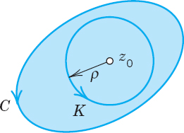
Fig. 357. Proof of Cauchy's integral formula

at each point of K. The length of K is 2πρ. Hence, by the ML-inequality in Sec. 14.1,
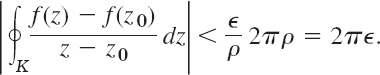
Since ![]() (> 0) can be chosen arbitrarily small, it follows that the last integral in (2) must have the value zero, and the theorem is proved.
(> 0) can be chosen arbitrarily small, it follows that the last integral in (2) must have the value zero, and the theorem is proved.
EXAMPLE 1 Cauchy's Integral Formula
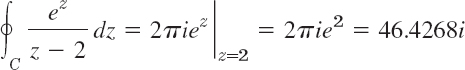
for any contour enclosing z0 = 2 (since ez is entire), and zero for any contour for which z0 = 2 lies outside (by Cauchy's integral theorem).

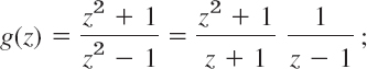
EXAMPLE 3 Integration Around Different Contours
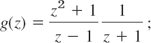
Integrate

counterclockwise around each of the four circles in Fig. 358.
Solution. g(z) is not analytic at −1 and 1. These are the points we have to watch for. We consider each circle separately.
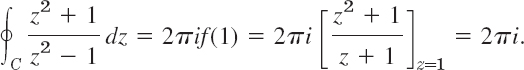
(a) The circle |z − 1| = 1 encloses the point z0 = 1 where g(z) is not analytic. Hence in (1) we have to write
thus

and (1) gives
(b) gives the same as (a) by the principle of deformation of path.
(c) The function g(z) is as before, but f(z) changes because we must take z0 = −1 (instead of 1). This gives a factor z − z0 = z + 1 in (1). Hence we must write
thus

Compare this for a minute with the previous expression and then go on:
(d) gives 0. Why?
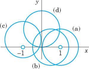
Fig. 358. Example 3
Multiply connected domains can be handled as in Sec. 14.2. For instance, if f(z) is analytic on C1 and C2 and in the ring-shaped domain bounded by C1 and C2 (Fig. 359) and z0 is any point in that domain, then

where the outer integral (over C1) is taken counterclockwise and the inner clockwise, as indicated in Fig. 359.

1–4 CONTOUR INTEGRATION
Integrate z2/(z2 − 1) by Cauchy's formula counterclockwise around the circle.
- |z + 1| = 1
- |z − 1 − i| = π/2
- |z + i| = 1.4
- |z + 5 − 5i| = 7
5–8 Integrate the given function around the unit circle.
- 5. (cos 3z)/(6z)
- 6. e2z/(πz − i)
- 7. z3/(2z − i)
- 8. (z2 sin z)/(4z − 1)
- 9. CAS EXPERIMENT. Experiment to find out to what extent your CAS can do contour integration. For this, use (a) the second method in Sec. 14.1 and (b) Cauchy's integral formula.
- 10. TEAM PROJECT. Cauchy's Integral Theorem. Gain additional insight into the proof of Cauchy's integral theorem by producing (2) with a contour enclosing z0 (as in Fig. 356) and taking the limit as in the text. Choose
and (c) another example of your choice.
11–19 FURTHER CONTOUR INTEGRALS
Integrate counterclockwise or as indicated. Show the details.
- 11.
 C: 4x2 + (y − 2)2 = 4
 - 12.
 C the circle with center −1 and radius 2
 - 13.
 C: |z − 1| = 2
 - 14.
 C: |z| = 0.6
 - 15.
 C the boundary of the square with vertices ±2, ±2, ±4i.
 - 16.
 C the boundary of the triangle with vertices 0 and ±1 + 2i.
 - 17.
 C: |z − i| = 1.4
 - 18.
 C consists of the boundaries of the squares with vertices ±3, ±3i counterclockwise and ±1, ±i clockwise (see figure).
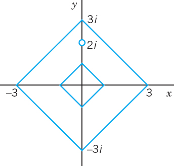
Problem 18
- 19.
 C consists of |z| = 2 counterclockwise and |z| = 1 clockwise.
 - 20. Show that
 dz = 0 for a simple closed path C enclosing z1 and z2, which are arbitrary.
14.4 Derivatives of Analytic Functions
As mentioned, a surprising fact is that complex analytic functions have derivatives of all orders. This differs completely from real calculus. Even if a real function is once differentiable we cannot conclude that it is twice differentiable nor that any of its higher derivatives exist. This makes the behavior of complex analytic functions simpler than real functions in this aspect. To prove the surprising fact we use Cauchy's integral formula.
THEOREM 1 Derivatives of an Analytic Function
If f(z) is analytic in a domain D, then it has derivatives of all orders in D, which are then also analytic functions in D. The values of these derivatives at a point z0 in D are given by the formulas


and in general

here C is any simple closed path in D that encloses z0 and whose full interior belongs to D; and we integrate counterclockwise around C (Fig. 360).

Fig. 360. Theorem 1 and its proof
COMMENT. For memorizing (1), it is useful to observe that these formulas are obtained formally by differentiating the Cauchy formula (1*) Sec. 14.3, under the integral sign with respect to z0
PROOF
We prove (1′), starting from the definition of the derivative

On the right we represent f(z0 + Δz) and f(z0) by Cauchy's integral formula:

We now write the two integrals as a single integral. Taking the common denominator gives the numerator f(z){z − z0 − [z − (z0 + Δz)]} = f(z) Δz, so that a factor Δz drops out and we get

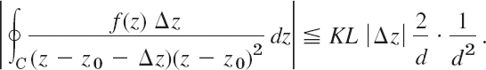
Clearly, we can now establish (1′) by showing that, as Δz → 0, the integral on the right approaches the integral in (1′). To do this, we consider the difference between these two integrals. We can write this difference as a single integral by taking the common denominator and simplifying the numerator (as just before). This gives
![]()
We show by the ML-inequality (Sec. 14.1) that the integral on the right approaches zero as Δz →0.
Being analytic, the function f(z) is continuous on C, hence bounded in absolute value, say, |f(z)| ![]() K. Let d be the smallest distance from z0 to the points of C (see Fig. 360). Then for all z on C,
K. Let d be the smallest distance from z0 to the points of C (see Fig. 360). Then for all z on C,

Furthermore, by the triangle inequality for all z on C we then also have
![]()
We now subtract |Δz| on both sides and let |Δz| ![]() d/2, so that −|Δz|
d/2, so that −|Δz| ![]() −d/2. Then
−d/2. Then
![]()
Let L be the length of C. If |Δz| ![]() d/2, then by the ML-inequality
d/2, then by the ML-inequality
This approaches zero as Δz →0. Formula (1′) is proved.
Note that we used Cauchy's integral formula (1*) Sec. 14.3, but if all we had known about f(z0) is the fact that it can be represented by (1*) Sec. 14.3, our argument would have established the existence of the derivative f′(z0) of f(z). This is essential to the continuation and completion of this proof, because it implies that (1″) can be proved by a similar argument, with f replaced by f′, and that the general formula (1) follows by induction.
Applications of Theorem 1
EXAMPLE 1 Evaluation of Line Integrals
From (1′), for any contour enclosing the point πi (counterclockwise)

From (1″), for any contour enclosing the point −i we obtain by counterclockwise integration
![]()

Cauchy's Inequality. Liouville's and Morera's Theorems
We develop other general results about analytic functions, further showing the versatility of Cauchy's integral theorem.
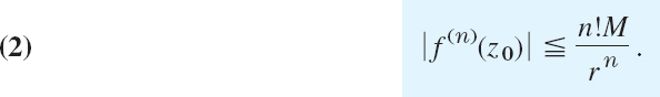
Cauchy's Inequality. Theorem 1 yields a basic inequality that has many applications. To get it, all we have to do is to choose for C in (1) a circle of radius r and center z0 and apply the ML-inequality (Sec. 14.1); with |f(z)| ![]() M on C we obtain from (1)
M on C we obtain from (1)

This gives Cauchy's inequality
To gain a first impression of the importance of this inequality, let us prove a famous theorem on entire functions (definition in Sec. 13.5). (For Liouville, see Sec. 11.5.)
If an entire function is bounded in absolute value in the whole complex plane, then this function must be a constant.
By assumption, |f(z)| is bounded, say, |f(z)| < K for all z. Using (2), we see that |f′(z0)| < K/r. Since f(z) is entire, this holds for every r, so that we can take r as large as we please and conclude that f′(z0) = 0. Since z0 is arbitrary, f′(z) = ux + ivx = 0 for all z (see (4) in Sec. 13.4), hence ux = vx = 0, and uy = vy = 0 by the Cauchy–Riemann equations. Thus u = const, v = const, and f = u + iv = const for all z. This completes the proof.
Another very interesting consequence of Theorem 1 is
THEOREM 3 Morera's2 Theorem (Converse of Cauchy's Integral Theorem)
If f(z) is continuous in a simply connected domain D and if

for every closed path in D, then f(z) is analytic in D.
PROOF
In Sec. 14.2 we showed that if f(z) is analytic in a simply connected domain D, then

is analytic in D and F′(z) = f(z). In the proof we used only the continuity of f(z) and the property that its integral around every closed path in D is zero; from these assumptions we concluded that F(z) is analytic. By Theorem 1, the derivative of F(z) is analytic, that is, f(z) is analytic in D, and Morera's theorem is proved.
This completes Chapter 14.
1–7 CONTOUR INTEGRATION. UNIT CIRCLE
Integrate counterclockwise around the unit circle.
8–19 INTEGRATION. DIFFERENT CONTOURS
Integrate. Show the details. Hint. Begin by sketching the contour. Why?
- 8.
 C the boundary of the square with vertices ±2, ±2i counterclockwise.
 - 9.
 C the ellipse 16x2 + y2 = 1 clockwise.
 - 10.
 C consists of |z| = 3 counterclockwise and |z| = 1 clockwise.
- 11.
 C: |z − i| = 2 counterclockwise.
 - 12.
 C: z − 3i| = 2 clockwise.
 - 13.
 C: |z − 3| = 2 counterclockwise.
 - 14.
 C the boundary of the square with vertices ±1.5, ±1.5i, counterclockwise.
 - 15.
 C consists of |z| = 6 counterclockwise |z − 3| = 2 and clockwise.
 - 16.
 C consists of |z −i| = 3 counterclockwise and |z| = 1 clockwise.
 - 17.
 C consists of |z| = 5 counterclockwise and
  clockwise.
 - 18.
 C: |z| = 1 counterclockwise, n integer.
 - 19.
 C: |z| = 1, counterclockwise.
 - 20. TEAM PROJECT. Theory on Growth
- Growth of entire functions. If f(z) is not a constant and is analytic for all (finite) z, and R and M are any positive real numbers (no matter how large), show that there exist values of z for which |z| > R and |f(z)| > M. Hint. Use Liouville's theorem.
- Growth of polynomials. If f(z) is a polynomial of degree n > 0 and M is an arbitrary positive real number (no matter how large), show that there exists a positive real number R such that for all |f(z)| > M for all |z| > R.
- Exponential function. Show that f(z) = ex has the property characterized in (a) but does not have that characterized in (b).
- Fundamental theorem of algebra.If f(z) is a polynomial in z, not a constant, then f(z) = 0 for at least one value of z. Prove this. Hint. Use (a).
CHAPTER 14 REVIEW QUESTIONS AND PROBLEMS
- What is a parametric representation of a curve? What is its advantage?
- What did we assume about paths of integration z = z(t)? What is
 geometrically?
 - State the definition of a complex line integral from memory.
- Can you remember the relationship between complex and real line integrals discussed in this chapter?
- How can you evaluate a line integral of an analytic function? Of an arbitrary continous complex function?
- What value do you get by counterclockwise integration of 1/z around the unit circle? You should remember this. It is basic.
- Which theorem in this chapter do you regard as most important? State it precisely from memory.
- What is independence of path? Its importance? State a basic theorem on independence of path in complex.
- What is deformation of path? Give a typical example.
- Don't confuse Cauchy's integral theorem (also known as Cauchy–Goursat theorem) and Cauchy's integral formula. State both. How are they related?
- What is a doubly connected domain? How can you extend Cauchy's integral theorem to it?
- What do you know about derivatives of analytic functions?
- How did we use integral formulas for derivatives in evaluating integrals?
- How does the situation for analytic functions differ with respect to derivatives from that in calculus?
- What is Liouville's theorem? To what complex functions does it apply?
- What is Morera's theorem?
- If the integrals of a function f(z) over each of the two boundary circles of an annulus D taken in the same sense have different values, can f(z) be analytic everywhere in D? Give reason.
- Is Im
 ? Give reason.
 - Is

- How would you find a bound for the left side in Prob. 19?
21–30 INTEGRATION
Integrate by a suitable method.
- 21. ∫C z sinh (z2)dz from 0 to πi/2.
- 22. ∫C (|z| + z)dz clockwise around the unit circle.
- 23. ∫C z−5ex dz counterclockwise around |z| = π.
- 24. ∫C Re z dz from 0 to 3 + 27i along y = x3.
- 25.
 clockwise around |z − 1| = 0.1
 - 26.
 from z = 0 horizontally to z = 2, then vertically upward to 2 + 2i.
 - 27.
 from 0 to 2 + 2i, shortest path.
 - 28.
 counterclockwise around
- 29.
 clockwise around |z − 1| = 2.5.
 - 30. ∫C sin z dz from 0 to (1 + i).
SUMMARY OF CHAPTER 14 Complex Integration
The complex line integral of a function f(z) taken over a path C is denoted by

If f(z) is analytic in a simply connected domain D, then we can evaluate (1) as in calculus by indefinite integration and substitution of limits, that is,

for every path C in D from a point z0 to a point z1 (see Sec. 14.1). These assumptions imply independence of path, that is, (2) depends only on z0 and z1 (and on f(z), of course) but not on the choice of C (Sec. 14.2). The existence of an F(z) such that F′(z) = f(z) is proved in Sec. 14.2 by Cauchy's integral theorem (see below).
A general method of integration, not restricted to analytic functions, uses the equation z = z(t) of C, where a ![]() t
t ![]() b,
b,

Cauchy's integral theorem is the most important theorem in this chapter. It states that if f(z) is analytic in a simply connected domain D, then for every closed path C in D (Sec. 14.2),

Under the same assumptions and for any z0 in D and closed path C in D containing z0 in its interior we also have Cauchy's integral formula
Furthermore, under these assumptions f(z) has derivatives of all orders in D that are themselves analytic functions in D and (Sec. 14.4)

This implies Morera's theorem (the converse of Cauchy's integral theorem) and Cauchy's inequality (Sec. 14.4), which in turn implies Liouville's theorem that an entire function that is bounded in the whole complex plane must be constant.
1ÉDOUARD GOURSAT (1858–1936), French mathematician who made important contributions to complex analysis and PDEs. Cauchy published the theorem in 1825. The removal of that condition by Goursat (see Transactions Amer. Math Soc., vol. 1, 1900) is quite important because, for instance, derivatives of analytic functions are also analytic. Because of this, Cauchy's integral theorem is also called Cauchy–Goursat theorem.
2GIACINTO MORERA (1856–1909), Italian mathematician who worked in Genoa and Turin.