
CHAPTER 25
Mathematical Statistics

In probability theory we set up mathematical models of processes that are affected by “chance.” In mathematical statistics or, briefly, statistics, we check these models against the observable reality. This is called statistical inference. It is done by sampling, that is, by drawing random samples, briefly called samples. These are sets of values from a much larger set of values that could be studied, called the population. An example is 10 diameters of screws drawn from a large lot of screws. Sampling is done in order to see whether a model of the population is accurate enough for practical purposes. If this is the case, the model can be used for predictions, decisions, and actions, for instance, in planning productions, buying equipment, investing in business projects, and so on.
Most important methods of statistical inference are estimation of parameters (Secs. 25.2), determination of confidence intervals (Sec. 25.3), and hypothesis testing (Sec. 25.4, 25.7, 25.8), with application to quality control (Sec. 25.5) and acceptance sampling (Sec. 25.6).
In the last section (25.9) we give an introduction to regression and correlation analysis, which concern experiments involving two variables.
Prerequisite: Chap. 24.
Sections that may be omitted in a shorter course: 25.5, 25.6, 25.8.
References, Answers to Problems, and Statistical Tables: App. 1 Part G, App. 2, App. 5.
25.1 Introduction. Random Sampling
Mathematical statistics consists of methods for designing and evaluating random experiments to obtain information about practical problems, such as exploring the relation between iron content and density of iron ore, the quality of raw material or manufactured products, the efficiency of air-conditioning systems, the performance of certain cars, the effect of advertising, the reactions of consumers to a new product, etc.
Random variables occur more frequently in engineering (and elsewhere) than one would think. For example, properties of mass-produced articles (screws, lightbulbs, etc.) always show random variation, due to small (uncontrollable!) differences in raw material or manufacturing processes. Thus the diameter of screws is a random variable X and we have nondefective screws, with diameter between given tolerance limits, and defective screws, with diameter outside those limits. We can ask for the distribution of X, for the percentage of defective screws to be expected, and for necessary improvements of the production process.
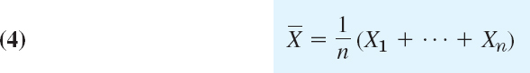
Samples are selected from populations—20 screws from a lot of of 1000, 100 of 5000 voters, 8 beavers in a wildlife conservation project—because inspecting the entire population would be too expensive, time-consuming, impossible or even senseless (think of destructive testing of lightbulbs or dynamite). To obtain meaningful conclusions, samples must be random selections. Each of the 1000 screws must have the same chance of being sampled (of being drawn when we sample), at least approximately. Only then will the sample mean ![]() (Sec. 24.1) of a sample of size n = 20 (or any other n) be a good approximation of the population mean μ (Sec. 24.6); and the accuracy of the approximation will generally improve with increasing n, as we shall see. Similarly for other parameters (standard deviation, variance, etc.).
(Sec. 24.1) of a sample of size n = 20 (or any other n) be a good approximation of the population mean μ (Sec. 24.6); and the accuracy of the approximation will generally improve with increasing n, as we shall see. Similarly for other parameters (standard deviation, variance, etc.).
Independent sample values will be obtained in experiments with an infinite sample space S (Sec. 24.2), certainly for the normal distribution. This is also true in sampling with replacement. It is approximately true in drawing small samples from a large finite population (for instance, 5 or 10 of 1000 items). However, if we sample without replacement from a small population, the effect of dependence of sample values may be considerable.
Random numbers help in obtaining samples that are in fact random selections. This is sometimes not easy to accomplish because there are many subtle factors that can bias sampling (by personal interviews, by poorly working machines, by the choice of nontypical observation conditions, etc.). Random numbers can be obtained from a random number generator in Maple, Mathematica, or other systems listed on p. 789. (The numbers are not truly random, as they would be produced in flipping coins or rolling dice, but are calculated by a tricky formula that produces numbers that do have practically all the essential features of true randomness. Because these numbers eventually repeat, they must not be used in cryptography, for example, where true randomness is required.)
EXAMPLE 1 Random Numbers from a Random Number Generator
To select a sample of size n = 10 from 80 given ball bearings, we number the bearings from 1 to 80. We then let the generator randomly produce 10 of the integers from 1 to 80 and include the bearings with the numbers obtained in our sample, for example.
![]()
or whatever.
Random numbers are also contained in (older) statistical tables.
Representing and processing data were considered in Sec. 24.1 in connection with frequency distributions. These are the empirical counterparts of probability distributions and helped motivating axioms and properties in probability theory. The new aspect in this chapter is randomness: the data are samples selected randomly from a population. Accordingly, we can immediately make the connection to Sec. 24.1, using stem-and-leaf plots, box plots, and histograms for representing samples graphically.
Also, we now call the mean ![]() in (5), Sec. 24.1, the sample mean
in (5), Sec. 24.1, the sample mean

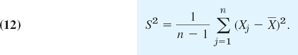
We call n the sample size, the variance s2 in (6), Sec. 24.1, the sample variance
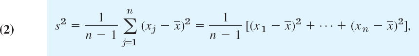
and its positive square root s the sample standard deviation. ![]() , s2, and s are called parametersof a sample; they will be needed throughout this chapter.
, s2, and s are called parametersof a sample; they will be needed throughout this chapter.
25.2 Point Estimation of Parameters
Beginning in this section, we shall discuss the most basic practical tasks in statistics and corresponding statistical methods to accomplish them. The first of them is point estimation of parameters, that is, of quantities appearing in distributions, such as p in the binomial distribution μ and σ and in the normal distribution.
A point estimate of a parameter is a number (point on the real line), which is computed from a given sample and serves as an approximation of the unknown exact value of the parameter of the population. An interval estimate is an interval (“confidence interval”) obtained from a sample; such estimates will be considered in the next section. Estimation of parameters is of great practical importance in many applications.
As an approximation of the mean μ of a population we may take the mean ![]() of a corresponding sample. This gives the estimate
of a corresponding sample. This gives the estimate ![]() for μ, that is,
for μ, that is,
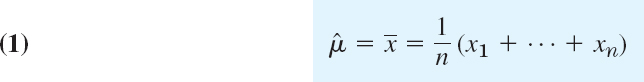
where n is the sample size. Similarly, an estimate ![]() for the variance of a population is the variance s2 of a corresponding sample, that is,
for the variance of a population is the variance s2 of a corresponding sample, that is,

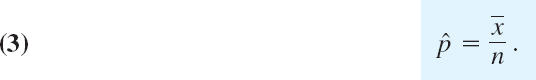
Clearly, (1) and (2) are estimates of parameters for distributions in which μ or σ2 appear explicity as parameters, such as the normal and Poisson distributions. For the binomial distribution, p = μ/n [see (3) in Sec. 24.7]. From (1) we thus obtain for p the estimate
We mention that (1) is a special case of the so-called method of moments. In this method the parameters to be estimated are expressed in terms of the moments of the distribution (see Sec. 24.6). In the resulting formulas, those moments of the distribution are replaced by the corresponding moments of the sample. This gives the estimates. Here the k th moment of a sample x1, …, xn is

Maximum Likelihood Method
Another method for obtaining estimates is the so-called maximum likelihood method of R. A. Fisher [Messenger Math. 41 (1912), 155–160]. To explain it, we consider a discrete (or continuous) random variable X whose probability function (or density) f(x) depends on a single parameter θ. We take a corresponding sample of n independent values x1, …,xn. Then in the discrete case the probability that a sample of size n consists precisely of those n values is

In the continuous case the probability that the sample consists of values in the small intervals xj ![]() x
x ![]() xj + Δx (j = 1, 2, …, n) is
xj + Δx (j = 1, 2, …, n) is
![]()
Since f(xj) depends on θ, the function l in (5) given by (4) depends on x1, …, xn and θ. We imagine x1, …, xn to be given and fixed. Then l is a function of which is called the likelihood function. The basic idea of the maximum likelihood method is quite simple, as follows. We choose that approximation for the unknown value of θ for which l is as large as possible. If l is a differentiable function of θ, a necessary condition for l to have a maximum in an interval (not at the boundary) is
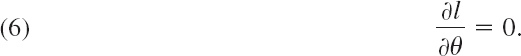
(We write a partial derivative, because l depends also on x1, …, xn.) A solution of (6) depending on x1, …, xn is called a maximum likelihood estimate for θ. We may replace (6) by
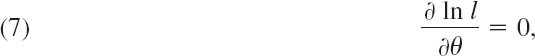
because f(xj) > 0, a maximum of l is in general positive, and ln l is a monotone increasing function of l. This often simplifies calculations.
Several Parameters. If the distribution of X involves r parameters θ1, …, θr, then instead of (6) we have the r conditions ∂l/∂θ1 = 0, …, ∂l/∂θr = 0, and instead of (7) we have

Find maximum likelihood estimates for θ1 = μ and θ2 = σ in the case of the normal distribution.
Solution. From (1), Sec. 24.8, and (4) we obtain the likelihood function
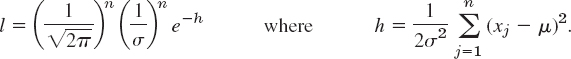
![]()
The first equation in (8) is ∂(ln l)/∂μ = 0, written out

The solution is the desired estimate ![]() for μ: we find
for μ: we find

The second equation in (8) is ∂(ln l)/∂σ = 0, written out

Replacing μ by ![]() and solving for σ2, we obtain the estimate
and solving for σ2, we obtain the estimate

which we shall use in Sec. 25.7. Note that this differs from (2). We cannot discuss criteria for the goodness of estimates but want to mention that for small n, formula (2) is preferable.
- Normal distribution. Apply the maximum likelihood method to the normal distribution with μ = 0.
- Find the maximum likelihood estimate for the parameter μ of a normal distribution with known variance
 .
. - Poisson distribution. Derive the maximum likelihood estimator for μ. Apply it to the sample (10, 25, 26, 17, 10, 4), giving numbers of minutes with 0–10, 11–20, 21–30, 31–40, 41–50, more than 50 fliers per minute, respectively, checking in at some airport check-in.
- Uniform distribution. Show that, in the case of the parameters a and b of the uniform distribution (see Sec. 24.6), the maximum likelihood estimate cannot be obtained by equating the first derivative to zero. How can we obtain maximum likelihood estimates in this case, more or less by using common sense?
- Binomial distribution. Derive a maximum likelihood estimate for p.
- Extend Prob. 5 as follows. Suppose that m times n trials were made and in the first n trials A happened k1 times, in the second n trials A happened k2 times, …, in the mth n trials A happened km times. Find a maximum likelihood estimate of p based on this information.
- Suppose that in Prob. 6 we made 3 times 4 trials and A happened 2, 3, 2 times, respectively. Estimate p.
- Geometric distribution. Let X = Number of independent trials until an event A occurs. Show that X has a geometric distribution, defined by the probability function f(x) = pqx−1, x = 1, 2, …, where p is the probability of A in a single trial and q = 1 p. Find the maximum likelihood estimate of p corresponding to a sample x1, x2, …, xn of observed values of X.
- In Prob. 8, show that f(1) + f(2) + … = 1 (as it should be!). Calculate independently of Prob. 8 the maximum likelihood of p in Prob. 8 corresponding to a single observed value of X.
- In rolling a die, suppose that we get the first “Six” in the 7th trial and in doing it again we get it in the 6th trial. Estimate the probability p of getting a “Six” in rolling that die once.
- Find the maximum likelihood estimate of θ in the density f(x) = θe−θx if x
 0 and f(x) = 0 if x < 0.
 - In Prob. 11, find the mean μ, substitute it in f(x), find the maximum likelihood estimate of μ, and show that it is identical with the estimate for μ which can be obtained from that for θ in Prob. 11.
- Compute
 in Prob. 11 from the sample 1.9, 0.4, 0.7, 0.6, 1.4. Graph the sample distribution function
  and the distribution function F(x) of the random variable, with
  , on the same axes. Do they agree reasonably well? (We consider goodness of fit systematically in Sec. 25.7.)
 - Do the same task as in Prob. 13 if the given sample is 0.4, 0.7, 0.2, 1.1, 0.1.
- CAS EXPERIMENT. Maximum Likelihood Estimates. (MLEs). Find experimentally how much MLEs can differ depending on the sample size. Hint. Generate many samples of the same size n, e.g., of the standardized normal distribution, and record
 and s2. Then increase n.
25.3 Confidence Intervals
Confidence intervals1 for an unknown parameter θ of some distribution (e.g., θ = μ) are intervals θ1 ![]() θ
θ ![]() θ2 that contain θ, not with certainty but with a high probability γ, which we can choose (95% and 99% are popular). Such an interval is calculated from a sample. γ = 95% means probability
θ2 that contain θ, not with certainty but with a high probability γ, which we can choose (95% and 99% are popular). Such an interval is calculated from a sample. γ = 95% means probability ![]() of being wrong—one of about 20 such intervals will not contain θ. Instead of writing θ1
of being wrong—one of about 20 such intervals will not contain θ. Instead of writing θ1 ![]() θ
θ ![]() θ2, we denote this more distinctly by writing
θ2, we denote this more distinctly by writing
![]()
Such a special symbol, CONF, seems worthwhile in order to avoid the misunderstanding that θ must lie between θ1 and θ2.
γ is called the confidence level, and θ1 and θ2 are called the lower and upper confidence limits. They depend on γ. The larger we choose γ, the smaller is the error probability 1 − γ, but the longer is the confidence interval. If γ → 1, then its length goes to infinity. The choice of γ depends on the kind of application. In taking no umbrella, a 5% chance of getting wet is not tragic. In a medical decision of life or death, a 5% chance of being wrong may be too large and a 1% chance of being wrong (γ = 99%) may be more desirable.
Confidence intervals are more valuable than point estimates (Sec. 25.2). Indeed, we can take the midpoint of (1) as an approximation of θ and half the length of (1) as an “error bound” (not in the strict sense of numerics, but except for an error whose probability we know).
θ1 and θ2 in (1) are calculated from a sample x1, …, xn. These are n observations of a random variable X. Now comes a standard trick. We regard x1, …, xn as single observations of n random variables X1, …, Xn (with the same distribution, namely, that of X). Then θ1 = θ1(x1, …, xn) and θ2 = θ2(x1, …, xn) in (1) are observed values of two random variables Θ1 = Θ1(X1, …, Xn) and Θ2 = Θ2(X1, …, Xn). The condition (1) involving γ can now be written
![]()
Let us see what all this means in concrete practical cases.
In each case in this section we shall first state the steps of obtaining a confidence interval in the form of a table, then consider a typical example, and finally justify those steps theoretically.
Confidence Interval for of the Normal Distribution with Known σ2
Table 25.1 Determination of a Confidence Interval for the Mean μ of a Normal Distribution with Known Variance σ2
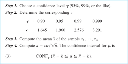
EXAMPLE 1 Confidence Interval for μ of the Normal Distribution with Known σ2
Determine a 95% confidence interval for the mean of a normal distribution with variance σ2 = 9, using a sample of n = 100 values with mean ![]() .
.
Solution. Step 1. γ = 0.95 is required. Step 2. The corresponding c equals 1.960; see Table 25.1.
Step 3. ![]() is given. Step 4. We need
is given. Step 4. We need ![]() . Hence
. Hence ![]() and the confidence interval is CONF0.95{4.412
and the confidence interval is CONF0.95{4.412 ![]() μ
μ ![]() 5.588}.
5.588}.
This is sometimes written μ = 5 ± 0.588, but we shall not use this notation, which can be misleading. With your CAS you can determine this interval more directly. Similarly for the other examples in this section.
Theory for Table 25.1. The method in Table 25.1 follows from the basic
Sum of Independent Normal Random Variables
Let X1, … Xn beindependent normal random variables each of which has mean μ and variance σ2. Then the following holds.
- The sum X1 + … + Xn is normal with mean nμ and variance nσ2.
- The following random variable
 is normal with mean μ and variance σ2/n.
- The following random variable Z is normal with mean 0 and variance 1.
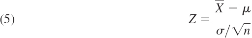
The statements about the mean and variance in (a) follow from Theorems 1 and 3 in Sec. 24.9. From this, and Theorem 2 in Sec. 24.6, we see that ![]() has the mean (1/n)nμ = μ and the variance (1/n)2nσ2 = σ2/n. This implies that Z has the mean 0 and variance 1, by Theorem 2(b) in Sec. 24.6. The normality of X1 + … + Xn is proved in Ref. [G3] listed in App. 1. This implies the normality of (4) and (5).
has the mean (1/n)nμ = μ and the variance (1/n)2nσ2 = σ2/n. This implies that Z has the mean 0 and variance 1, by Theorem 2(b) in Sec. 24.6. The normality of X1 + … + Xn is proved in Ref. [G3] listed in App. 1. This implies the normality of (4) and (5).
Derivation of (3) in Table 25.1. Sampling from a normal distribution gives independent sample values (see Sec. 25.1), so that Theorem 1 applies. Hence we can choose γ and then determine c such that

For the value γ = 0.95 we obtain z(D) = 1.960 from Table A8 in App. 5, as used in Example 1. For γ = 0.9, 0.99, 0.999 we get the other values of c listed in Table 25.1. Finally, all we have to do is to convert the inequality in (6) into one for μ and insert observed values obtained from the sample. We multiply −c ![]() Z
Z ![]() c by −1 and then by
c by −1 and then by ![]() , writing
, writing ![]() (as in Table 25.1),
(as in Table 25.1),

Adding ![]() gives
gives ![]() or
or
![]()
Inserting the observed value ![]() of
of ![]() gives (3). Here we have regarded x1, …, xn as single observations of X1, …, Xn (the standard trick!), so that x1 + … + xn is an observed value of X1 + … + Xn and
gives (3). Here we have regarded x1, …, xn as single observations of X1, …, Xn (the standard trick!), so that x1 + … + xn is an observed value of X1 + … + Xn and ![]() is an observed value of
is an observed value of ![]() . Note further that (7) is of the form (2) with
. Note further that (7) is of the form (2) with ![]() and
and ![]() .
.
EXAMPLE 2 Sample Size Needed for a Confidence Interval of Prescribed Length
How large must n be in Example 1 if we want to obtain a 95% confidence interval of length L = 0.4?
Solution. The interval (3) has the length ![]() Solving for n, we obtain
Solving for n, we obtain
![]()
In the present case the answer is n = (2 · 13960 · 3/0.42 ≈ 870.
Figure 526 shows how L decreases as n increases and that for γ = 99% the confidence interval is substantially longer than for γ = 95% (and the same sample size n).

Fig. 526. Length of the confidence interval (3) (measured in multiples of σ as a function of the sample size n for γ = 95% and γ = 99%
Confidence Interval for μ of the Normal Distribution with Unknown σ2
In practice σ2 is frequently unknown. Then the method in Table 25.1 does not help and the whole theory changes, although the steps of determining a confidence interval for μ remain quite similar. They are shown in Table 25.2. We see that k differs from that in Table 25.1, namely, the sample standard deviation s has taken the place of the unknown standard deviation σ of the population. And c now depends on the sample size n and must be determined from Table A9 in App. 5 or from your CAS. That table lists values z for given values of the distribution function (Fig. 527)

of the t-distribution. Here, m (= 1, 2, …) is a parameter, called the number of degrees of freedom of the distribution (abbreviated d.f.). In the present case, m = n − 1; see Table 25.2. The constant Km is such that F(∞) = 1. By integration it turns out that ![]() , where Γ is the gamma function (see (24) in App. A3.1).
, where Γ is the gamma function (see (24) in App. A3.1).
Table 25.2 Determination of a Confidence Interval for the Mean μ of a Normal Distribution with Unknown Variance σ2
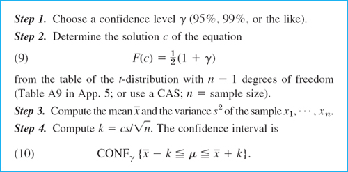
Figure 528 compares the curve of the density of the t-distribution with that of the normal distribution. The latter is steeper. This illustrates that Table 25.1 (which uses more information, namely, the known value of σ2) yields shorter confidence intervals than Table 25.2. This is confirmed in Fig. 529, which also gives an idea of the gain by increasing the sample size.
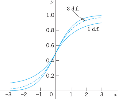
Fig. 527. Distribution functions of the t-distribution with 1 and 3 d.f. and of the standardized normal distribution (steepest curve)

Fig. 528. Densities of the t-distribution with 1 and 3 d.f. and of the standardized normal distribution

Fig. 529. Ratio of the lengths L′ and L of the confidence intervals (10) and (3) with γ = 95% and γ = 99% as a function of the sample size n for equal s and σ
EXAMPLE 3 Confidence Interval for μ of the Normal Distribution with Unknown σ2
Five independent measurements of the point of inflammation (flash point) of Diesel oil (D-2) gave the values (in °F) 144 147 146 142 144. Assuming normality, determine a 99% confidence interval for the mean.
Solution. Step 1. γ = 0.99 is required.
Step 2. ![]() , and Table A9 in App. 5 with n − 1 = 4 d.f. gives c = 4.60.
, and Table A9 in App. 5 with n − 1 = 4 d.f. gives c = 4.60.
Step 3. ![]() .
.
Step 4. ![]() . The confidence interval is CONF0.99{140.5
. The confidence interval is CONF0.99{140.5 ![]() μ
μ ![]() 148.7}.
148.7}.
If the variance σ2 were known and equal to the sample variance s2, thus σ2 = 3.8, then Table 25.1 would give ![]() and CONF0.99 {142.35
and CONF0.99 {142.35 ![]() μ
μ ![]() 146.85}. We see that the present interval is almost twice as long as that obtained from Table 25.1 (with σ2 = 3.8). Hence for small samples the difference is considerable! See also Fig. 529.
146.85}. We see that the present interval is almost twice as long as that obtained from Table 25.1 (with σ2 = 3.8). Hence for small samples the difference is considerable! See also Fig. 529.
Theory for Table 25.2. For deriving (10) in Table 25.2 we need from Ref. [G3]
THEOREM 2 Student's t-Distribution
Let X1, …, Xn be independent normal random variables with the same mean μ and the same variance σ2. Then the random variable
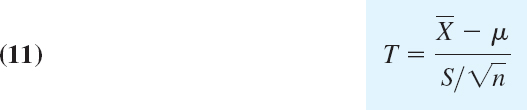
has a t-distribution [see (8)] with n − 1 degrees of freedom (d.f.); here ![]() is given by (4) and
is given by (4) and
Derivation of (10). This is similar to the derivation of (3). We choose a number γ between 0 and 1 and determine a number c from Table A9 in App. 5 with n − 1 d.f. (or from a CAS) such that
![]()
Since the t-distribution is symmetric, we have
![]()
and (13) assumes the form (9). Substituting (11) into (13) and transforming the result as before, we obtain
![]()
where
![]()
By inserting the observed values ![]() of
of ![]() and s2 of S2 into (14) we finally obtain (10).
and s2 of S2 into (14) we finally obtain (10).
Confidence Interval for the Variance σ2
of the Normal Distribution
Table 25.3 shows the steps, which are similar to those in Tables 25.1 and 25.2.
Table 25.3 Determination of a Confidence Interval for the Variance σ2 of a Normal Distribution, Whose Mean Need Not Be Known

EXAMPLE 4 Confidence Interval for the Variance of the Normal Distribution
Determine a 95% confidence interval (16) for the variance, using Table 25.3 and a sample (tensile strength of sheet steel in kg/mm2, rounded to integer values)
![]()
Solution. Step 1. γ = 0.95 is required.
Step 2. For n − 1 = 13 we find
![]()
Step 3. 13s2 = 326.9.
Step 4. 13s2/c1 = 65.25, 13s2/c2 = 13.21.
The confidence interval is
![]()
This is rather large, and for obtaining a more precise result, one would need a much larger sample.
Theory for Table 25.3. In Table 25.1 we used the normal distribution, in Table 25.2 the t-distribution, and now we shall use the x2-distribution (chi-square distribution), whose distribution function is F(z) = 0 if z < 0 and
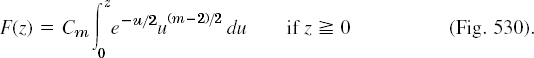
The parameter m (= 1, 2, …) is called the number of degrees of freedom (d.f.), and
![]()
Note that the distribution is not symmetric (see also Fig. 531).
For deriving (16) in Table 25.3 we need the following theorem.

Fig. 530. Distribution function of the chi-square distribution with 2, 3, 5 d.f.
THEOREM 3 Chi-Square Distribution
Under the assumptions in Theorem 2 the random variable
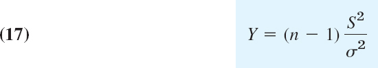
with S2 given by (12) has a chi-square distribution with n − 1 degrees of freedom.
Proof in Ref. [G3], listed in App. 1.

Fig. 531. Density of the chi-square distribution with 2, 3, 5 d.f.
Derivation of (16). This is similar to the derivation of (3) and (10). We choose a number γ between 0 and 1 and determine c1 and c2 from Table A10, App. 5, such that [see (15)]
![]()
![]()
Transforming c1 ![]() Y
Y ![]() c2 with Y given by (17) into an inequality for σ2, we obtain
c2 with Y given by (17) into an inequality for σ2, we obtain
![]()
By inserting the observed value s2 of S2 we obtain (16).
Confidence Intervals for Parameters
of Other Distributions
The methods in Tables 25.1–25.3 for confidence intervals for μ and σ2 are designed for the normal distribution. We now show that they can also be applied to other distributions if we use large samples.
We know that if X1, …, Xn are independent random variables with the same mean μ and the same variance σ2, then their sum Yn = X1 + … + Xn has the following properties.
(A) Yn has the mean nμ and the variance nσ2 (by Theorems 1 and 3 in Sec. 24.9).
(B) If those variables are normal, then Yn is normal (by Theorem 1).
If those random variables are not normal, then (B) is not applicable. However, for large n the random variable Yn is still approximately normal. This follows from the central limit theorem, which is one of the most fundamental results in probability theory.
THEOREM 4 Central Limit Theorem
Let X1, …, Xn, … be independent random variables that have the same distribution function and therefore the same mean μ and the same variance σ2. Let Yn = X1 + … + Xn. Then the random variable
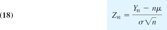
is asymptotically normal with mean 0 and variance 1; that is, the distribution function Fn(x) of Zn satisfies
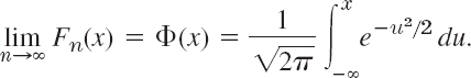
A proof can be found in Ref. [G3] listed in App. 1.
Hence, when applying Tables 25.1–25.3 to a nonnormal distribution, we must use sufficiently large samples. As a rule of thumb, if the sample indicates that the skewness of the distribution (the asymmetry; see Team Project 20(d), Problem Set 24.6) is small, use at least n = 20 for the mean and at least n = 50 for the variance.
- Why are interval estimates generally more useful than point estimates?
2–6 MEAN (VARIANCE KNOWN)
- 2. Find a 95% confidence interval for the mean of a normal population with standard deviation 4.00 from the sample 39, 51, 49, 43, 57, 59. Does that interval get longer or shorter if we take γ = 0.99 instead of 0.95? By what factor?
- 3. By what factor does the length of the interval in Prob. 2 change if we double the sample size?
- 4. Determine a 95% confidence interval for the mean μ of a normal population with variance σ2 = 16, using a sample of size 200 with mean 74.81.
- 5. What sample size would be needed for obtaining a 95% confidence interval (3) of length 2σ? Of length σ?
- 6. What sample size is needed to obtain a 99% confidence interval of length 2.0 for the mean of a normal population with variance 25? Use Fig. 526. Check by calculation.
MEAN (VARIANCE UNKNOWN)
- 7. Find a 95% confidence interval for the percentage of cars on a certain highway that have poorly adjusted brakes, using a random sample of 800 cars stopped at a roadblock on that highway, 126 of which had poorly adjusted brakes.
- 8. K. Pearson result. Find a 99% confidence interval for p in the binomial distribution from a classical result by K. Pearson, who in 24,000 trials of tossing a coin obtained 12,012 Heads. Do you think that the coin was fair?
9–11 Find a confidence interval for the mean of a normal population from the sample:
- 9. Copper content (%) of brass 66, 66, 65, 64, 66, 67, 64, 65, 63, 64, 65, 63, 64
- 10. Melting point (°C) of aluminum 660, 667, 654, 663, 662
- 11. Knoop hardness of diamond 9500, 9800, 9750, 9200, 9400, 9550
- 12. CAS EXPERIMENT. Confidence Intervals. Obtain 100 samples of size 10 of the standardized normal distribution. Calculate from them and graph the corresponding 95% confidence intervals for the mean and count how many of them do not contain 0. Does the result support the theory? Repeat the whole experiment, compare and comment.
13–17 VARIANCE
Find a 95% confidence interval for the variance of a normal population from the sample:
- 13. Length of 20 bolts with sample mean 20.2 cm and sample variance 0.04 cm2
- 14. Carbon monoxide emission (grams per mile) of a certain type of passenger car (cruising at 55 mph): 17.3, 17.8, 18.0, 17.7, 18.2, 17.4, 17.6, 18.1
- 15. Mean energy (keV) of delayed neutron group (Group 3, half-life 6.2 s) for uranium U235 fission: a sample of 100 values with mean 442.5 and variance 9.3
- 16. Ultimate tensile strength (k psi) of alloy steel (Maraging H) at room temperature: 251, 255, 258, 253, 253, 252, 250, 252, 255, 256
- 17. The sample in Prob. 9
- 18. If X1 and X2 are independent normal random variables with mean 14 and 8 and variance 2 and 5, respectively, what distribution does 3 X1 − X2 have? Hint. Use Team Project 14(g) in Sec. 24.8.
- 19. A machine fills boxes weighing Y lb with X lb of salt, where X and Y are normal with mean 100 lb and 5 lb and standard deviation 1 lb and 0.5 lb, respectively. What percent of filled boxes weighing between 104 lb and 106 lb are to be expected?
- 20. If the weight X of bags of cement is normally distributed with a mean of 40 kg and a standard deviation of 2 kg, how many bags can a delivery truck carry so that the probability of the total load exceeding 2000 kg will be 5%?
25.4 Testing of Hypotheses. Decisions
The ideas of confidence intervals and of tests2 are the two most important ideas in modern statistics. In a statistical test we make inference from sample to population through testing a hypothesis, resulting from experience or observations, from a theory or a quality requirement, and so on. In many cases the result of a test is used as a basis for a decision, for instance, to buy (or not to buy) a certain model of car, depending on a test of the fuel efficiency (and other tests, of course), to apply some medication, depending on a test of its effect; to proceed with a marketing strategy, depending on a test of consumer reactions, etc.
Let us explain such a test in terms of a typical example and introduce the corresponding standard notions of statistical testing.
EXAMPLE 1 Test of a Hypothesis. Alternative. Significance Level α
We want to buy 100 coils of a certain kind of wire, provided we can verify the manufacturer's claim that the wire has a breaking limit μ μ0 = 200 lb (or more). This is a test of the hypothesis (also called null hypothesis) μ = μ0 = 200. We shall not buy the wire if the (statistical) test shows that actually μ = μ1 < μ0, the wire is weaker, the claim does not hold. μ1 is called the alternative (or alternative hypothesis) of the test. We shall accept the hypothesis if the test suggests that it is true, except for a small error probability α, called the significance level of the test. Otherwise we reject the hypothesis. Hence α is the probability of rejecting a hypothesis although it is true. The choice of α is up to us. 5% and 1% are popular values.
For the test we need a sample. We randomly select 25 coils of the wire, cut a piece from each coil, and determine the breaking limit experimentally. Suppose that this sample of n = 25 values of the breaking limit has the mean ![]() (somewhat less than the claim!) and the standard deviation s = 6 lb.
(somewhat less than the claim!) and the standard deviation s = 6 lb.
At this point we could only speculate whether this difference 197 − 200 = −3 is due to randomness, is a chance effect, or whether it is significant, due to the actually inferior quality of the wire. To continue beyond speculation requires probability theory, as follows.
We assume that the breaking limit is normally distributed. (This assumption could be tested by the method in Sec. 25.7. Or we could remember the central limit theorem (Sec. 25.3) and take a still larger sample.) Then

in (11), Sec. 25.3, with μ = μ0 has a t-distribution with n − 1 degrees of freedom (n − 1 = 24 for our sample). Also ![]() and s = 6 are observed values of
and s = 6 are observed values of ![]() and S to be used later. We can now choose a significance level, say, α = 5%. From Table A9 in App. 5 or from a CAS we then obtain a critical value c such that P(T
and S to be used later. We can now choose a significance level, say, α = 5%. From Table A9 in App. 5 or from a CAS we then obtain a critical value c such that P(T ![]() c) = α = 5%. For
c) = α = 5%. For ![]() the table gives
the table gives ![]() , so that
, so that ![]() because of the symmetry of the distribution (Fig. 532).
because of the symmetry of the distribution (Fig. 532).
We now reason as follows—this is the crucial idea of the test. If the hypothesis is true, we have a chance of only α (= 5%) that we observe a value t of T (calculated from a sample) that will fall between −∞ and −1.71. Hence, if we nevertheless do observe such a t, we assert that the hypothesis cannot be true and we reject it. Then we accept the alternative. If, however, t ![]() c, we accept the hypothesis.
c, we accept the hypothesis.
A simple calculation finally gives ![]() as an observed value of T. Since −2.5 < −1.71, we reject the hypothesis (the manufacturer's claim) and accept the alternative μ = μ1 < 200, the wire seems to be weaker than claimed.
as an observed value of T. Since −2.5 < −1.71, we reject the hypothesis (the manufacturer's claim) and accept the alternative μ = μ1 < 200, the wire seems to be weaker than claimed.
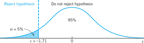
Fig. 532. t-distribution in Example 1
This example illustrates the steps of a test:
- Formulate the hypothesis θ = θ0 to be tested. (θ0 = μ0 in the example.)
- Formulate an alternative θ = θ1. (θ1 = μ1 in the example.)
- Choose a significance level α (5%, 1%, 0.1%).
4. Use a random variable ![]() whose distribution depends on the hypothesis and on the alternative, and this distribution is known in both cases. Determine a critical value c from the distribution of
whose distribution depends on the hypothesis and on the alternative, and this distribution is known in both cases. Determine a critical value c from the distribution of ![]() , assuming the hypothesis to be true. (In the example,
, assuming the hypothesis to be true. (In the example, ![]() and c is, obtained from P(T
and c is, obtained from P(T ![]() c) = α.)
c) = α.)
5. Use a sample x1, …, xn to determine an observed value ![]() of
of ![]() . (t in the example.)
. (t in the example.)
6. Accept or reject the hypothesis, depending on the size of ![]() relative to c. (t < c in the example, rejection of the hypothesis.)
relative to c. (t < c in the example, rejection of the hypothesis.)
Two important facts require further discussion and careful attention. The first is the choice of an alternative. In the example, μ1 < μ0, but other applications may require μ1 > μ0 or μ1 ≠ μ0. The second fact has to do with errors. We know that α (the significance level of the test) is the probability of rejecting a true hypothesis. And we shall discuss the probability β of accepting a false hypothesis.
One-Sided and Two-Sided Alternatives (Fig. 533)
Let θ be an unknown parameter in a distribution, and suppose that we want to test the hypothesis θ = θ0. Then there are three main kinds of alternatives, namely,
![]()
![]()
![]()
(1) and (2) are one-sided alternatives, and (3) is a two-sided alternative.
We call rejection region (or critical region) the region such that we reject the hypothesis if the observed value in the test falls in this region. In ![]() the critical c lies to the right of θ0 because so does the alternative. Hence the rejection region extends to the right. This is called a right-sided test. In
the critical c lies to the right of θ0 because so does the alternative. Hence the rejection region extends to the right. This is called a right-sided test. In ![]() the critical c lies to the left of θ0 (as in Example 1), the rejection region extends to the left, and we have a left-sided test (Fig. 533, middle part). These are one-sided tests. In
the critical c lies to the left of θ0 (as in Example 1), the rejection region extends to the left, and we have a left-sided test (Fig. 533, middle part). These are one-sided tests. In ![]() we have two rejection regions. This is called a two-sided test (Fig. 533, lower part).
we have two rejection regions. This is called a two-sided test (Fig. 533, lower part).

Fig. 533. Test in the case of alternative (1) (upper part of the figure), alternative (2) (middle part), and alternative (3)
All three kinds of alternatives occur in practical problems. For example, (1) may arise if θ0 is the maximum tolerable inaccuracy of a voltmeter or some other instrument. Alternative (2) may occur in testing strength of material, as in Example 1. Finally, θ0 in (3) may be the diameter of axle-shafts, and shafts that are too thin or too thick are equally undesirable, so that we have to watch for deviations in both directions.
Errors in Tests
Tests always involve risks of making false decisions:
- Rejecting a true hypothesis (Type I error).
α = Probability of making a Type I error.
- Accepting a false hypothesis (Type II error).
β = Probability of making a Type II error.
Clearly, we cannot avoid these errors because no absolutely certain conclusions about populations can be drawn from samples. But we show that there are ways and means of choosing suitable levels of risks, that is, of values α and β. The choice of α depends on the nature of the problem (e.g., a small risk α = 1% is used if it is a matter of life or death).
Let us discuss this systematically for a test of a hypothesis θ = θ0 against an alternative that is a single number θ1, for simplicity. We let θ1 > θ0, so that we have a right-sided test. For a left-sided or a two-sided test the discussion is quite similar.
We choose a critical c > θ0 (as in the upper part of Fig. 533, by methods discussed below). From a given sample x1, …, xn we then compute a value
![]()
with a suitable g (whose choice will be a main point of our further discussion; for instance, take g = (x1 + … + xn)/n in the case in which θ is the mean). If ![]() , we reject the hypothesis. If
, we reject the hypothesis. If ![]() , we accept it. Here, the value
, we accept it. Here, the value ![]() can be regarded as an observed value of the random variable
can be regarded as an observed value of the random variable
![]()
because xj may be regarded as an observed value of Xj,j = 1, …, n. In this test there are two possibilities of making an error, as follows.
Type I Error (see Table 25.4). The hypothesis is true but is rejected (hence the alternative is accepted) because Θ assumes a value ![]() . Obviously, the probability of making such an error equals
. Obviously, the probability of making such an error equals
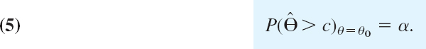
α is called the significance level of the test, as mentioned before.
Type II Error (see Table 25.4). The hypothesis is false but is accepted because ![]() assumes a value
assumes a value ![]() . The probability of making such an error is denoted by β thus
. The probability of making such an error is denoted by β thus
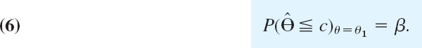
η = 1 − β is called the power of the test. Obviously, the power η is the probability of avoiding a Type II error.
Table 25.4 Type I and Type II Errors in Testing a Hypothesis θ = θ0 Against an Alternative θ = θ1

Formulas (5) and (6) show that both α and β depend on c, and we would like to choose c so that these probabilities of making errors are as small as possible. But the important Figure 534 shows that these are conflicting requirements because to let α decrease we must shift c to the right, but then β increases. In practice we first choose α (5%, sometimes 1%), then determine c, and finally compute β. If β is large so that the power η = 1 − β is small, we should repeat the test, choosing a larger sample, for reasons that will appear shortly.
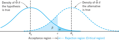
Fig. 534. Illustration of Type I and II errors in testing a hypothesis θ = θ0 against an alternative θ = θ1 (> θ0, right-sided test)
If the alternative is not a single number but is of the form (1)–(3), then β becomes a function of θ. This function β(θ) is called the operating characteristic (OC) of the test and its curve the OC curve. Clearly, in this case η = 1 − β also depends on θ. This function η(θ) is called the power function of the test. (Examples will follow.)
Of course, from a test that leads to the acceptance of a certain hypothesis θ0, it does not follow that this is the only possible hypothesis or the best possible hypothesis. Hence the terms “not reject” or “fail to reject” are perhaps better than the term “accept.”
Test for μ of the Normal Distribution with Known σ2
The following example explains the three kinds of hypotheses.
EXAMPLE 2 Test for the Mean of the Normal Distribution with Known Variance
Let X be a normal random variable with variance σ2 = 9. Using a sample of size n = 10 with mean ![]() , test the hypothesis μ = μ0 = 24 against the three kinds of alternatives, namely,
, test the hypothesis μ = μ0 = 24 against the three kinds of alternatives, namely,
![]()
Solution. We choose the significance level α = 0.05. An estimate of the mean will be obtained from
![]()
If the hypothesis is true, ![]() is normal with mean μ = 24 and variance σ2/n = 0.9, see Theorem 1, Sec. 25.3.
is normal with mean μ = 24 and variance σ2/n = 0.9, see Theorem 1, Sec. 25.3.
Hence we may obtain the critical value c from Table A8 in App. 5.
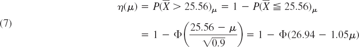
Case (a). Right-Sided Test. We determine c from ![]() , that is,
, that is,
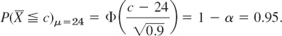
Table A8 in App. 5 gives ![]() , and c = 25.56, which is greater than μ0, as in the upper part of Fig. 533. If
, and c = 25.56, which is greater than μ0, as in the upper part of Fig. 533. If ![]() , the hypothesis is accepted. If
, the hypothesis is accepted. If ![]() , it is rejected. The power function of the test is (Fig. 535)
, it is rejected. The power function of the test is (Fig. 535)
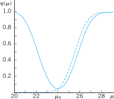
Fig. 535. Power function η(μ) in Example 2, case (a) (dashed) and case (c)
Case (b). Left-Sided Test. The critical value c is obtained from the equation

Table A8 in App. 5 yields c = 24 − 1.56 = 22.44. If ![]() , we accept the hypothesis. If
, we accept the hypothesis. If ![]() , we reject it. The power function of the test is
, we reject it. The power function of the test is

Case (c). Two-Sided Test. Since the normal distribution is symmetric, we choose c1 and c2 equidistant from μ = 24, say, c1 = 24 − k and c2 = 24 + k, and determine k from

Table A8 in App. 5 gives ![]() , hence k = 1.86. This gives the values c1 = 24 − 1.86 = 22.14 and c2 = 24 + 1.86 = 25.86 If
, hence k = 1.86. This gives the values c1 = 24 − 1.86 = 22.14 and c2 = 24 + 1.86 = 25.86 If ![]() is not smaller than c1 and not greater than c2, we accept the hypothesis. Otherwise we reject it. The power function of the test is (Fig. 535)
is not smaller than c1 and not greater than c2, we accept the hypothesis. Otherwise we reject it. The power function of the test is (Fig. 535)
![]()
Consequently, the operating characteristic β(μ) = 1 − η(μ) (see before) is (Fig. 536)
![]()
If we take a larger sample, say, of size n = 100 (instead of 10), then σ2/n = 0.09 (instead of 0.9) and the critical values are c1 = 23.41 and c2 = 24.29, as can be readily verified. Then the operating characteristic of the test is

Figure 536 shows that the corresponding OC curve is steeper than that for n = 10. This means that the increase of n has led to an improvement of the test. In any practical case, n is chosen as small as possible but so large that the test brings out deviations between μ and μ0 that are of practical interest. For instance, if deviations of ±2 units are of interest, we see from Fig. 536 that n = 10 is much too small because when μ = 24 − 2 = 22 or μ = 24 + 2 = 26 β is almost 50%. On the other hand, we see that n = 100 is sufficient for that purpose.

Fig. 536. Curves of the operating characteristic (OC curves) in Example 2, case (c), for two different sample sizes n
Test for μ When σ2 Is Unknown, and for σ2
EXAMPLE 3 Test for the Mean of the Normal Distribution with Unknown Variance
The tensile strength of a sample of n = 16 manila ropes (diameter 3 in.) was measured. The sample mean was ![]() , and the sample standard deviation was s = 115 kg (N. C. Wiley, 41st Annual Meeting of the American Society for Testing Materials). Assuming that the tensile strength is a normal random variable, test the hypothesis μ0 = 4500 kg against the alternative μ1 = 4400 kg. Here μ0 may be a value given by the manufacturer, while μ1 may result from previous experience.
, and the sample standard deviation was s = 115 kg (N. C. Wiley, 41st Annual Meeting of the American Society for Testing Materials). Assuming that the tensile strength is a normal random variable, test the hypothesis μ0 = 4500 kg against the alternative μ1 = 4400 kg. Here μ0 may be a value given by the manufacturer, while μ1 may result from previous experience.
Solution. We choose the significance level α = 5%. If the hypothesis is true, it follows from Theorem 2 in Sec. 25.3, that the random variable

has a t-distribution with n − 1 = 15 d.f. The test is left-sided. The critical value c is obtained from P(T < c)μ0 = α = 0.05. Table A9 in App. 5 gives c = −1.75. As an observed value of T we obtain from the sample t = (4482 − 4500)/(115/4) = −0.626. We see that t > c and accept the hypothesis. For obtaining numeric values of the power of the test, we would need tables called noncentral Student t-tables; we shall not discuss this question here.
EXAMPLE 4 Test for the Variance of the Normal Distribution
Using a sample of size n = 15 and sample variance s2 = 13 from a normal population, test the hypothesis ![]() against the alternative
against the alternative ![]() .
.
Solution. We choose the significance level α = 5%. If the hypothesis is true, then

has a chi-square distribution with n − 1 = 14 d.f. by Theorem 3, Sec. 25.3. From
![]()
and Table A10 in App. 5 with 14 degrees of freedom we obtain c = 23.68. This is the critical value of Y. Hence to ![]() there corresponds the critical value c* = 0.714 · 23.68 = 16.91. Since s2 < c*, we accept the hypothesis.
there corresponds the critical value c* = 0.714 · 23.68 = 16.91. Since s2 < c*, we accept the hypothesis.
If the alternative is true, the random variable ![]() has a chi-square distribution with 14 d.f. Hence our test has the power
has a chi-square distribution with 14 d.f. Hence our test has the power
![]()
From a more extensive table of the chi-square distribution (e.g. in Ref. [G3] or [G8]) or from your CAS, you see that η ≈ 62%. Hence the Type II risk is very large, namely, 38%. To make this risk smaller, we would have to increase the sample size.
Comparison of Means and Variances
EXAMPLE 5 Comparison of the Means of Two Normal Distributions
Using a sample ![]() from a normal distribution with unknown mean μx and a sample
from a normal distribution with unknown mean μx and a sample ![]() from another normal distribution with unknown mean μy, we want to test the hypothesis that the means are equal, μx = μy, against an alternative, say, μx > μy. The variances need not be known but are assumed to be equal.3
from another normal distribution with unknown mean μy, we want to test the hypothesis that the means are equal, μx = μy, against an alternative, say, μx > μy. The variances need not be known but are assumed to be equal.3
Two cases of comparing means are of practical importance:
Case A. The samples have the same size.Furthermore, each value of the first sample corresponds to precisely one value of the other, because corresponding values result from the same person or thing (paired comparison)—for example, two measurements of the same thing by two different methods or two measurements from the two eyes of the same person. More generally, they may result from pairs of similar individuals or things, for example, identical twins, pairs of used front tires from the same car, etc. Then we should form the differences of corresponding values and test the hypothesis that the population corresponding to the differences has mean 0, using the method in Example 3. If we have a choice, this method is better than the following.
Case B.The two samples are independent and not necessarily of the same size. Then we may proceed as follows. Suppose that the alternative is μx > μy. We choose a significance level α. Then we compute the sample means ![]() and
and ![]() as well as
as well as ![]() and
and ![]() , where
, where ![]() and
and ![]() are the sample variances. Using Table A9 in App. 5 with n1 + n2 − 2 degrees of freedom, we now determine c from
are the sample variances. Using Table A9 in App. 5 with n1 + n2 − 2 degrees of freedom, we now determine c from
![]()
We finally compute

It can be shown that this is an observed value of a random variable that has a t-distribution with n1 + n2 −2 degrees of freedom, provided the hypothesis is true. If t0 ![]() c, the hypothesis is accepted. If t0 > c, it is rejected.
c, the hypothesis is accepted. If t0 > c, it is rejected.
If the alternative is μx ≠ μy then (10) must be replaced by
![]()
Note that for samples of equal size n1 = n2 = n, formula (11) reduces to
To illustrate the computations, let us consider the two samples ![]() and
and ![]() given by
given by

showing the relative output of tin plate workers under two different working conditions [J. J. B. Worth, Journal of Industrial Engineering 9, 249–253). Assuming that the corresponding populations are normal and have the same variance, let us test the hypothesis μx = μy against the alternative μx ≠ μy. (Equality of variances will be tested in the next example.)
Solution. We find
![]()
We choose the significance level α = 5%. From (10*) with 0.5α = 2.5%, 1 − 0.5α = 97.5% and Table A9 in App. 5 with 14 degrees of freedom we obtain. c1 = −2.14 and c2 = 2.14. Formula (12) with n = 8 gives the value
![]()
Since c1 ![]() t0
t0 ![]() c2, we accept the hypothesis μx = μy that under both conditions the mean output is the same.
c2, we accept the hypothesis μx = μy that under both conditions the mean output is the same.
Case A applies to the example because the two first sample values correspond to a certain type of work, the next two were obtained in another kind of work, etc. So we may use the differences
![]()
of corresponding sample values and the method in Example 3 to test the hypothesis μ = 0, where μ is the mean of the population corresponding to the differences. As a logical alternative we take μ ≠ 0. The sample mean is ![]() , and the sample variance is s2 = 45.696. Hence
, and the sample variance is s2 = 45.696. Hence
![]()
From P(T ![]() c1) = 2.5%, P(T
c1) = 2.5%, P(T ![]() c2) = 97.5% and Table A9 in App. 5 with n − 1 = 7 degrees of freedom we obtain c1 = −2.36, c2 = 2.36 and reject the hypothesis because t = 3.19 does not lie between c1 and c2. Hence our present test, in which we used more information (but the same samples), shows that the difference in output is significant.
c2) = 97.5% and Table A9 in App. 5 with n − 1 = 7 degrees of freedom we obtain c1 = −2.36, c2 = 2.36 and reject the hypothesis because t = 3.19 does not lie between c1 and c2. Hence our present test, in which we used more information (but the same samples), shows that the difference in output is significant.
EXAMPLE 6 Comparison of the Variance of Two Normal Distributions
Using the two samples in the last example, test the hypothesis ![]() ; assume that the corresponding populations are normal and the nature of the experiment suggests the alternative
; assume that the corresponding populations are normal and the nature of the experiment suggests the alternative ![]() .
.
Solution. We find ![]() . We choose the significance level α = 5%. Using P(V
. We choose the significance level α = 5%. Using P(V ![]() c) = 1 − α = 95% and Table A11 in App. 5, with (n1 −1, n2 − 1) = (7, 7) degrees of freedom, we determine c = 3.79. We finally compute
c) = 1 − α = 95% and Table A11 in App. 5, with (n1 −1, n2 − 1) = (7, 7) degrees of freedom, we determine c = 3.79. We finally compute ![]() . Since ν0
. Since ν0 ![]() c, we accept the hypothesis. If ν0 < c, we would reject it.
c, we accept the hypothesis. If ν0 < c, we would reject it.
This test is justified by the fact that is an observed value of a random variable that has a so-called F-distribution with (n1 − 1, n2 − 1) degrees of freedom, provided the hypothesis is true. (Proof in Ref. [G3] listed in App. 1.) The F-distribution with (m, n) degrees of freedom was introduced by R. A. Fisher4 and has the distribution function F(z) = 0 if z < 0 and

where ![]() . (For Γ see App. A 3.1.)
. (For Γ see App. A 3.1.)
This long section contained the basic ideas and concepts of testing, along with typical applications and you may perhaps want to review it quickly before going on, because the next sections concern an adaptation of these ideas to tasks of great practical importance and resulting tests in connection with quality control, acceptance (or rejection) of goods produced, and so on.
- From memory: Make a list of the three types of alternatives, each with a typical example of your own.
- Make a list of methods in this section, each with the distribution needed in testing.
- Test μ = 0 against μ > 0, assuming normality and using the sample 0, 1, −1, 3, −8, 6, 1 (deviations of the azimuth [multiples of 0.01 radian] in some revolution of a satellite). Choose α = 5%.
- In one of his classical experiments Buffon obtained 2048 heads in tossing a coin 4040 times. Was the coin fair?
- Do the same test as in Prob. 4, using a result by K. Pearson, who obtained 6019 heads in 12,000 trials.
- Assuming normality and known variance σ2 = 9, test the hypothesis μ = 60.0 against the alternative μ = 57.0 using a sample of size 20 with mean
 and choosing α = 5%.
 - How does the result in Prob. 6 change if we use a smaller sample, say, of size 5, the other data (
 , α = 5%, etc.) remaining as before?
 - Determine the power of the test in Prob. 6.
- What is the rejection region in Prob. 6 in the case of a two-sided test with α = 5%?
- CAS EXPERIMENT. Tests of Means and Variances. (a) Obtain 100 samples of size 10 each from the normal distribution with mean 100 and variance 25. For each sample, test the hypothesis μ0 = 100 against the alternative μ1 > 100 at the level of α = 10%. Record the number of rejections of the hypothesis. Do the whole experiment once more and compare.
(b) Set up a similar experiment for the variance of a normal distribution and perform it 100 times.
- 11. A firm sells oil in cans containing 5000 g oil per can and is interested to know whether the mean weight differs significantly from 5000 g at the 5% level, in which case the filling machine has to be adjusted. Set up a hypothesis and an alternative and perform the test, assuming normality and using a sample of 50 fillings with mean 4990 g and standard deviation 20 g.
- If a sample of 25 tires of a certain kind has a mean life of 37,000 miles and a standard deviation of 5000 miles, can the manufacturer claim that the true mean life of such tires is greater than 35,000 miles? Set up and test a corresponding hypothesis at the 5% level, assuming normality.
- If simultaneous measurements of electric voltage by two different types of voltmeter yield the differences (in volts) 0.4, −0.6, 0.2, 0.0, 1.0, 1.4, 0.4, 1.6, can we assert at the 5% level that there is no significant difference in the calibration of the two types of instruments? Assume normality.
- If a standard medication cures about 75% of patients with a certain disease and a new medication cured 310 of the first 400 patients on whom it was tried, can we conclude that the new medication is better? Choose α = 5%. First guess. Then calculate.
- Suppose that in the past the standard deviation of weights of certain 100.0-oz packages filled by a machine was 0.8 oz. Test the hypothesis H0: σ = 0.8 against the alternative H1: σ > 0.8 (an undesirable increase), using a sample of 20 packages with standard deviation 1.0 oz and assuming normality. Choose α = 5%.
- Suppose that in operating battery-powered electrical equipment, it is less expensive to replace all batteries at fixed intervals than to replace each battery individually when it breaks down, provided the standard deviation of the lifetime is less than a certain limit, say, less than 5 hours. Set up and apply a suitable test, using a sample of 28 values of lifetimes with standard deviation s = 3.5 hours and assuming normality: choose α = 5%.
- Brand A gasoline was used in 16 similar automobiles under identical conditions. The corresponding sample of 16 values (miles per gallon) had mean 19.6 and standard deviation 0.4. Under the same conditions, high-power brand B gasoline gave a sample of 16 values with mean 20.2 and standard deviation 0.6. Is the mileage of B significantly better than that of A? Test at the 5% level; assume normality. First guess. Then calculate.
- The two samples 70, 80, 30, 70, 60, 80 and 140, 120, 130, 120, 120, 130, 120 are values of the differences of temperatures (°C) of iron at two stages of casting, taken from two different crucibles. Is the variance of the first population larger than that of the second? Assume normality. Choose α = 5%.
- Show that for a normal distribution the two types of errors in a test of a hypothesis H0: μ = μ0 against an alternative H1: μ = μ1 can be made as small as one pleases (not zero!) by taking the sample sufficiently large.
- Test for equality of population means against the alternative that the means are different assuming normality, choosing α = 5% and using two samples of sizes 12 and 18, with mean 10 and 14, respectively, and equal standard deviation 3.
25.5 Quality Control
The ideas on testing can be adapted and extended in various ways to serve basic practical needs in engineering and other fields. We show this in the remaining sections for some of the most important tasks solvable by statistical methods. As a first such area of problems, we discuss industrial quality control, a highly successful method used in various industries.
No production process is so perfect that all the products are completely alike. There is always a small variation that is caused by a great number of small, uncontrollable factors and must therefore be regarded as a chance variation. It is important to make sure that the products have required values (for example, length, strength, or whatever property may be essential in a particular case). For this purpose one makes a test of the hypothesis that the products have the required property, say, μ = μ0, where μ0 is a required value. If this is done after an entire lot has been produced (for example, a lot of 100,000 screws), the test will tell us how good or how bad the products are, but it it obviously too late to alter undesirable results. It is much better to test during the production run. This is done at regular intervals of time (for example, every hour or half-hour) and is called quality control. Each time a sample of the same size is taken, in practice 3 to 10 times. If the hypothesis is rejected, we stop the production and look for the cause of the trouble.
If we stop the production process even though it is progressing properly, we make a Type I error. If we do not stop the process even though something is not in order, we make a Type II error (see Sec. 25.4). The result of each test is marked in graphical form on what is called a control chart. This was proposed by W. A. Shewhart in 1924 and makes quality control particularly effective.
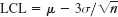
Control Chart for the Mean
An illustration and example of a control chart is given in the upper part of Fig. 537. This control chart for the mean shows the lower control limit LCL, the center control line CL, and the upper control limit UCL. The two control limits correspond to the critical values c1 and c2 in case (c) of Example 2 in Sec. 25.4. As soon as a sample mean falls outside the range between the control limits, we reject the hypothesis and assert that the production process is “out of control”; that is, we assert that there has been a shift in process level. Action is called for whenever a point exceeds the limits.
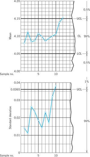
Fig. 537. Control charts for the mean (upper part of figure) and the standard deviation in the case of the samples on p. 1089
If we choose control limits that are too loose, we shall not detect process shifts. On the other hand, if we choose control limits that are too tight, we shall be unable to run the process because of frequent searches for nonexistent trouble. The usual significance level is α = 1%. From Theorem 1 in Sec. 25.3 and Table A8 in App. 5 we see that in the case of the normal distribution the corresponding control limits for the mean are

Here σ is assumed to be known. If σ is unknown, we may compute the standard deviations of the first 20 or 30 samples and take their arithmetic mean as an approximation of σ. The broken line connecting the means in Fig. 537 is merely to display the results.
Additional, more subtle controls are often used in industry. For instance, one observes the motions of the sample means above and below the centerline, which should happen frequently. Accordingly, long runs (conventionally of length 7 or more) of means all above (or all below) the centerline could indicate trouble.
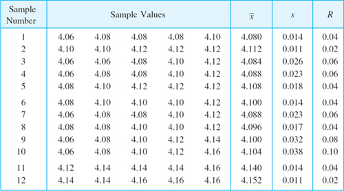
Table 25.5 Twelve Samples of Five Values Each (Diameter of Small Cylinders, Measured in Millimeters)
Control Chart for the Variance
In addition to the mean, one often controls the variance, the standard deviation, or the range. To set up a control chart for the variance in the case of a normal distribution, we may employ the method in Example 4 of Sec. 25.4 for determining control limits. It is customary to use only one control limit, namely, an upper control limit. Now from Example 4 of Sec. 25.4 we have ![]() , where, because of our normality assumption, the random variable Y has a chi-square distribution with n − 1 degrees of freedom. Hence the desired control limit is
, where, because of our normality assumption, the random variable Y has a chi-square distribution with n − 1 degrees of freedom. Hence the desired control limit is

where c is obtained from the equation
![]()
and the table of the chi-square distribution (Table A10 in App. 5) with n − 1 degrees of freedom (or from your CAS); here α (5% or 1% say) is the probability that in a properly running process an observed value s2 of S2 is greater than the upper control limit.
If we wanted a control chart for the variance with both an upper control limit UCL and a lower control limit LCL, these limits would be

where c1 and c2 are obtained from Table A10 with n − 1 d.f. and the equations
![]()
Control Chart for the Standard Deviation
To set up a control chart for the standard deviation, we need an upper control limit
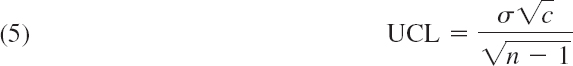
obtained from (2). For example, in Table 25.5 we have n = 5. Assuming that the corresponding population is normal with standard deviation σ = 0.02 and choosing α = 1% we obtain from the equation
![]()
and Table A10 in App. 5 with 4 degrees of freedom the critical value c = 13.28 and from (5) the corresponding value
![]()
which is shown in the lower part of Fig. 537.
A control chart for the standard deviation with both an upper and a lower control limit is obtained from (3).
Control Chart for the Range
Instead of the variance or standard deviation, one often controls the range R (= largest sample value minus smallest sample value). It can be shown that in the case of the normal distribution, the standard deviation σ is proportional to the expectation of the random variable R* for which R is an observed value, say, σ = λnE(R*) where the factor of proportionality λn depends on the sample size n and has the values

Since R depends on two sample values only, it gives less information about a sample than s does. Clearly, the larger the sample size n is, the more information we lose in using R instead of s. A practical rule is to use s when n is larger than 10.
- Suppose a machine for filling cans with lubricating oil is set so that it will generate fillings which form a normal population with mean 1 gal and standard deviation 0.02 gal. Set up a control chart of the type shown in Fig. 537 for controlling the mean, that is, find LCL and UCL, assuming that the sample size is 4.
- Three-sigma control chart. Show that in Prob. 1, the requirement of the significance level α = 0.3% leads to
 and
and 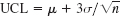 , and find the corresponding numeric values.
 - What sample size should we choose in Prob. 1 if we want LCL and UCL somewhat closer together, say, UCL − LCL = 0.02, without changing the significance level?
- What effect on UCL − LCL does it have if we double the sample size? If we switch from α = 1% to α = 5%?
- How should we change the sample size in controlling the mean of a normal population if we want UCL − LCL to decrease to half its original value?
- Graph the means of the following 10 samples (thickness of gaskets, coded values) on a control chart for means, assuming that the population is normal with mean 5 and standard deviation 1.16.
- Graph the ranges of the samples in Prob. 6 on a control chart for ranges.
- Graph λn = σ/E(R*) as a function of n. Why is λn a monotone decreasing function of n?
- Eight samples of size 2 were taken from a lot of screws. The values (length in inches) are

Assuming that the population is normal with mean 3.500 and variance 0.0004 and using (1), set up a control chart for the mean and graph the sample means on the chart.
- Attribute control charts. Fifteen samples of size 100 were taken from a production of containers. The numbers of defectives (leaking containers) in those samples (in the order observed) were

From previous experience it was known that the average fraction defective is p = 4% provided that the process of production is running properly. Using the binomial distribution, set up a fraction defective chart (also called a p-chart), that is, choose the

LCL = 0 and determine the UCL for the fraction defective (in percent) by the use of 3-sigma limits, where σ2 is the variance of the random variable

Is the process under control?
- Number of defectives. Find formulas for the UCL, CL, and LCL (corresponding to 3σ-limits) in the case of a control chart for the number of defectives, assuming that, in a state of statistical control, the fraction of defectives is p.
- CAS PROJECT. Control Charts. (a) Obtain 100 samples of 4 values each from the normal distribution with mean 8.0 and variance 0.16 and their means, variances, and ranges.
(b) Use these samples for making up a control chart for the mean.
(c) Use them on a control chart for the standard deviation.
(d) Make up a control chart for the range.
(e) Describe quantitative properties of the samples that you can see from those charts (e.g., whether the 3 corresponding process is under control, whether the quantities observed vary randomly, etc.).
- Since the presence of a point outside control limits for the mean indicates trouble, how often would we be making the mistake of looking for nonexistent trouble if we used (a) 1-sigma limits, (b) 2-sigma limits? Assume normality.
- What LCL and UCL should we use instead of (1) if, instead of
 , we use the sum x1 + … + xn of the sample values? Determine these limits in the case of Fig. 537.
 - Number of defects per unit. A so-called c-chart or defects-per-unit chart is used for the control of the number X of defects per unit (for instance, the number of defects per 100 meters of paper, the number of missing rivets in an airplane wing, etc.). (a) Set up formulas for CL and LCL, UCL corresponding to μ ± 3σ, assuming that X has a Poisson distribution.
(b) Compute CL, LCL, and UCL in a control process of the number of imperfections in sheet glass; assume that this number is 3.6 per sheet on the average when the process is in control.
25.6 Acceptance Sampling
Acceptance sampling is usually done when products leave the factory (or in some cases even within the factory). The standard situation in acceptance sampling is that a producer supplies to a consumer (a buyer or wholesaler) a lot of N items (a carton of screws, for instance). The decision to accept or reject the lot is made by determining the number x of defectives (= defective items) in a sample of size n from the lot. The lot is accepted if x ![]() c, where c is called the acceptance number, giving the allowable number of defectives. If x > c, the consumer rejects the lot. Clearly, producer and consumer must agree on a certain sampling plan giving n and c.
c, where c is called the acceptance number, giving the allowable number of defectives. If x > c, the consumer rejects the lot. Clearly, producer and consumer must agree on a certain sampling plan giving n and c.
From the hypergeometric distribution we see that the event A: “Accept the lot” has probability (see Sec. 24.7)
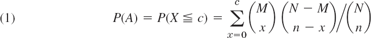
where M is the number of defectives in a lot of N items. In terms of the fraction defective θ = M/N we can write (1) as

P(A; θ) can assume n + 1 values corresponding to θ = 0, 1/N, 2/N, …, N/N; here, n and c are fixed. A monotone smooth curve through these points is called the operating characteristic curve (OC curve) of the sampling plan considered.
Suppose that certain tool bits are packaged 20 to a box, and the following sampling plan is used. A sample of two tool bits is drawn, and the corresponding box is accepted if and only if both bits in the sample are good. In this case, N = 20, n = 2, c = 0, and (2) takes the form (a factor 2 drops out)

The values of P(A, θ) for θ = 0, 1/20, 2/20, …, 20/20 and the resulting OC curve are shown in Fig. 538. (Verify!)

Fig. 538. OC curve of the sampling plan with n = 2 and c = 0 for lots of size N = 20

Fig. 539. OC curve in Example 2
In most practical cases θ will be small (less than 10%). Then if we take small samples compared to N, we can approximate (2) by the Poisson distribution (Sec. 24.7); thus

EXAMPLE 2 Sampling Plan. Poisson Distribution
Suppose that for large lots the following sampling plan is used. A sample of size n = 20 is taken. If it contains not more than one defective, the lot is accepted. If the sample contains two or more defectives, the lot is rejected. In this plan, we obtain from (3)
![]()
The corresponding OC curve is shown in Fig. 539.
Errors in Acceptance Sampling
We show how acceptance sampling fits into general test theory (Sec. 25.4) and what this means from a practical point of view. The producer wants the probability α of rejecting

Fig. 540. OC curve, producer's and consumer's risks
an acceptable lot (a lot for which θ does not exceed a certain number θ0 on which the two parties agree) to be small. θ0 is called the acceptable quality level (AQL). Similarly, the consumer (the buyer) wants the probability β of accepting an unacceptable lot (a lot for which θ is greater than or equal to some θ1) to be small. θ1 is called the lot tolerance percent defective (LTPD) or the rejectable quality level (RQL). α is called producer's risk. It corresponds to a Type I error in Sec. 25.4. β is called consumer's risk and corresponds to a Type II error. Figure 540 shows an example. We see that the points (θ0, 1 − α) and (θ1, β) lie on the OC curve. It can be shown that for large lots we can choose θ0, θ1 (> θ0), α, β and then determine n and c such that the OC curve runs very close to those prescribed points. Table 25.6 shows the analogy between acceptance sampling and hypothesis testing in Sec. 25.4.
Table 25.6 Acceptance Sampling and Hypothesis Testing
| Acceptance Sampling | Hypothesis Testing |
| Acceptable quality level (AQL) θ = θ0 | Hypothesis θ = θ0 |
| Lot tolerance percent defectives (LTPD) θ = θ1 | Alternative θ = θ1 |
| Allowable number of defectives c | Critical value c |
| Producer's risk α of rejecting a lot with θ |
Probability α of making a Type I error with (significance level) |
| Consumer's risk β of accepting a lot with θ |
Probability β of making a Type II error |
Rectification
Rectification of a rejected lot means that the lot is inspected item by item and all defectives are removed and replaced by nondefective items. (This may be too expensive if the lot is cheap; in this case the lot may be sold at a cut-rate price or scrapped.) If a production turns out 100θ% defectives, then in K lots of size N each, KNθ of the KN items are defectives. Now KP(A; θ) of these lots are accepted. These contain KPNθ defectives, whereas the rejected and rectified lots contain no defectives, because of the rectification. Hence after the rectification the fraction defective in all K lots equals KPNθ/KN. This is called the average outgoing quality (AOQ); thus

Figure 541 shows an example. Since AOQ(0) = 0 and P(A; 1) = 0, the AOQ curve has a maximum at some θ = θ*, giving the average outgoing quality limit (AOQL). This is the worst average quality that may be expected to be accepted under rectification.
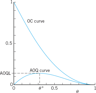
Fig. 541. OC curve and AOQ curve for the sampling plan in Fig. 538
- Lots of kitchen knives are inspected by a sampling plan that uses a sample of size 20 and the acceptance number c = 1. What is the probability of accepting a lot with 1%, 2%, 10% defectives (knives with dull blades)? Use Table A6 of the Poisson distribution in App. 5. Graph the OC curve.
- What happens in Prob. 1 if the sample size is increased to 50? First guess. Then calculate. Graph the OC curve and compare.
- How will the probabilities in Prob. 1 with n = 20 change (up or down) if we decrease c to zero? First guess.
- What are the producer's and consumer's risks in Prob. 1 if the AQL is 2% and the RQL is 15%?
- Lots of copper pipes are inspected according to a sample plan that uses sample size 25 and acceptance number 1. Graph the OC curve of the plan, using the Poisson approximation. Find the producer's risk if the AQL is 1.5%.
- Graph the AOQ curve in Prob. 5. Determine the AOQL, assuming that rectification is applied.
- In Example 1 in the text, what are the producer's and consumer's risks if the AQL is 0.1 and the RQL is 0.6?
- What happens in Example 1 in the text if we increase the sample size to n = 3, leaving the other data as before? Compute P(A; 0.1) and P(A; 0.2) and compare with Example 1.
- Graph and compare sampling plans with c = 1 and increasing values of n, say, n = 2, 3, 4. (Use the binomial distribution.)
- Find the binomial approximation of the hypergeometric distribution in Example 1 in the text and compare the approximate and the accurate values.
- Samples of 3 fuses are drawn from lots and a lot is accepted if in the corresponding sample we find no more than 1 defective fuse. Criticize this sampling plan. In particular, find the probability of accepting a lot that is 50% defective. (Use the binomial distribution (7), Sec. 24.7.)
- If in a sampling plan for large lots of spark plugs, the sample size is 100 and we want the AQL to be and the producer's risk 2%, what acceptance number c should we choose? (Use the normal approximation of the binomial distribution in Sec. 24.8.)
- What is the consumer's risk in Prob. 12 if we want the RQL to be 12%? Use c = 9 from the answer of Prob. 12.
- A lot of batteries for wrist watches is accepted if and only if a sample of 20 contains at most 1 defective. Graph the OC and AOQ curves. Find AOQL. [Use (3).]
- Graph the OC curve and the AOQ curve for the single sampling plan for large lots with n = 5 and c = 0, and find the AOQL.
25.7 Goodness of Fit. X2-Test
To test for goodness of fit means that we wish to test that a certain function F(x) is the distribution function of a distribution from which we have a sample x1, …, xn. Then we test whether the sample distribution function ![]() defined by
defined by
![]()
fits F(x) “sufficiently well.” If this is so, we shall accept the hypothesis that F(x) is the distribution function of the population; if not, we shall reject the hypothesis.
This test is of considerable practical importance, and it differs in character from the tests for parameters μ, σ2, etc.) considered so far.
To test in that fashion, we have to know how much ![]() can differ from F(x) if the hypothesis is true. Hence we must first introduce a quantity that measures the deviation of
can differ from F(x) if the hypothesis is true. Hence we must first introduce a quantity that measures the deviation of ![]() from F(x), and we must know the probability distribution of this quantity under the assumption that the hypothesis is true. Then we proceed as follows. We determine a number c such that, if the hypothesis is true, a deviation greater than c has a small preassigned probability. If, nevertheless, a deviation greater than c occurs, we have reason to doubt that the hypothesis is true and we reject it. On the other hand, if the deviation does not exceed c, so that
from F(x), and we must know the probability distribution of this quantity under the assumption that the hypothesis is true. Then we proceed as follows. We determine a number c such that, if the hypothesis is true, a deviation greater than c has a small preassigned probability. If, nevertheless, a deviation greater than c occurs, we have reason to doubt that the hypothesis is true and we reject it. On the other hand, if the deviation does not exceed c, so that ![]() approximates F(x) sufficiently well, we accept the hypothesis. Of course, if we accept the hypothesis, this means that we have insufficient evidence to reject it, and this does not exclude the possibility that there are other functions that would not be rejected in the test. In this respect the situation is quite similar to that in Sec. 25.4.
approximates F(x) sufficiently well, we accept the hypothesis. Of course, if we accept the hypothesis, this means that we have insufficient evidence to reject it, and this does not exclude the possibility that there are other functions that would not be rejected in the test. In this respect the situation is quite similar to that in Sec. 25.4.
Table 25.7 shows a test of that type, which was introduced by R. A. Fisher. This test is justified by the fact that if the hypothesis is true, then ![]() is an observed value of a random variable whose distribution function approaches that of the chi-square distribution with K − 1 degrees of freedom (or K − r − 1 degrees of freedom if r parameters are estimated) as n approaches infinity. The requirement that at least five sample values lie in each interval in Table 25.7 results from the fact that for finite n that random variable has only approximately a chi-square distribution. A proof can be found in Ref. [G3] listed in App. 1. If the sample is so small that the requirement cannot be satisfied, one may continue with the test, but then use the result with caution.
is an observed value of a random variable whose distribution function approaches that of the chi-square distribution with K − 1 degrees of freedom (or K − r − 1 degrees of freedom if r parameters are estimated) as n approaches infinity. The requirement that at least five sample values lie in each interval in Table 25.7 results from the fact that for finite n that random variable has only approximately a chi-square distribution. A proof can be found in Ref. [G3] listed in App. 1. If the sample is so small that the requirement cannot be satisfied, one may continue with the test, but then use the result with caution.
Table 25.7 Chi-square Test for the Hypothesis ThatF(x) is the Distribution Function of a Population from Which a Sample x1, …, xn is Taken
Table 25.8 Sample of 100 Values of the Splitting Tensile Strength (lb/in.2) of Concrete Cylinders
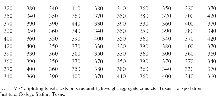
Test whether the population from which the sample in Table 25.8 was taken is normal.
Solution. Table 25.8 shows the values (column by column) in the order obtained in the experiment. Table 25.9 gives the frequency distribution and Fig. 542 the histogram. It is hard to guess the outcome of the test—does the histogram resemble a normal density curve sufficiently well or not?
The maximum likelihood estimates for μ and σ2 are ![]() and
and ![]() . The computation in Table 25.10 yields
. The computation in Table 25.10 yields ![]() . It is very interesting that the interval 375…385 contributes over 50% of
. It is very interesting that the interval 375…385 contributes over 50% of ![]() . From the histogram we see that the corresponding frequency looks much too small. The second largest contribution comes from 395…405, and the histogram shows that the frequency seems somewhat too large, which is perhaps not obvious from inspection.
. From the histogram we see that the corresponding frequency looks much too small. The second largest contribution comes from 395…405, and the histogram shows that the frequency seems somewhat too large, which is perhaps not obvious from inspection.
Table 25.9 Frequency Table of the Sample in Table 25.8
We choose α = 5%. Since K = 10 and we estimated r = 2 parameters we have to use Table A10 in App. 5 with K − r − 1 = 7 degrees of freedom. We find c = 14.07 as the solution of p(x2 ![]() c) = 95%. Since
c) = 95%. Since ![]() , we accept the hypothesis that the population is normal.
, we accept the hypothesis that the population is normal.

Fig. 542. Frequency histogram of the sample in Table 25.8
Table 25.10 Computations in Example 1
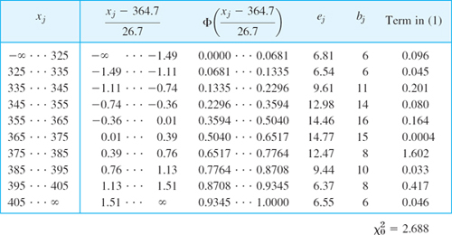
- Verify the calculations in Example 1 of the text.
- If it is known that 25% of certain steel rods produced by a standard process will break when subjected to a load of 5000 lb, can we claim that a new, less expensive process yields the same breakage rate if we find that in a sample of 80 rods produced by the new process, 27 rods broke when subjected to that load? (Use α = 5%.)
- If 100 flips of a coin result in 40 heads and 60 tails, can we assert on the 5% level that the coin is fair?
- If in 10 flips of a coin we get the same ratio as in Prob. 3 (4 heads and 6 tails), is the conclusion the same as in Prob. 3? First conjecture, then compute.
- Can you claim, on a 5% level, that a die is fair if 60 trials give 1, …, 6 with absolute frequencies 10, 13, 9, 11, 9, 8?
- Solve Prob. 5 if rolling a die 180 times gives 33, 27, 29, 35, 25, 31.
- If a service station had served 60, 49, 56, 46, 68, 39 cars from Monday through Friday between 1 P.M. and 2 P.M., can one claim on a 5% level that the differences are due to randomness? First guess. Then calculate.
- A manufacturer claims that in a process of producing drill bits, only 2.5% of the bits are dull. Test the claim against the alternative that more than 2.5% of the bits are dull, using a sample of 400 bits containing 17 dull ones. Use α = 5%.
- In a table of properly rounded function values, even and odd last decimals should appear about equally often. Test this for the 90 values of J1(x) in Table A1 in App. 5.
- TEAM PROJECT. Difficulty with Random Selection. 77 students were asked to choose 3 of the integers 11, 12, 13, …, 30 completely arbitrarily. The amazing result was as follows.

If the selection were completely random, the following hypotheses should be true.
- The 20 numbers are equally likely.
- The 10 even numbers together are as likely as the 10 odd numbers together.
- The 6 prime numbers together have probability 0.3 and the 14 other numbers together have probability 0.7. Test these hypotheses, using α = 5%. Design further experiments that illustrate the difficulties of random selection.
- CAS EXPERIMENT. Random Number Generator. Check your generator experimentally by imitating results of n trials of rolling a fair die, with a convenient n (e.g., 60 or 300 or the like). Do this many times and see whether you can notice any “nonrandomness” features, for example, too few Sixes, too many even numbers, etc., or whether your generator seems to work properly. Design and perform other kinds of checks.
- Test for normality at the 1% level using a sample of n = 79 (rounded) values x (tensile strength [kg>mm2] of steel sheets of 0.3 mm thickness). a = a(x) = absolute frequency. (Take the first two values together, also the last three, to get K = 5.)
- Mendel's pathbreaking experiments. In a famous plant-crossing experiment, the Austrian Augustinian father Gregor Mendel (1822–1884) obtained 355 yellow and 123 green peas. Test whether this agrees with Mendel's theory according to which the ratio should be 3:1.
- Accidents in a foundry. Does the random variable X = Number of accidents per week have a Poisson distribution if, within 50 weeks, 33 were accident-free, 1 accident occurred in 11 of the 50 weeks, 2 in 6 of the weeks, and more than 2 accidents in no week? Choose α = 5%.
- Radioactivity. Rutherford-Geiger experiments. Using the given sample, test that the corresponding population has a Poisson distribution. x is the number of alpha particles per 7.5-s intervals observed by E. Rutherford and H. Geiger in one of their classical experiments in 1910, and a(x) is the absolute frequency (= number of time periods during which exactly x particles were observed). Use α = 5%.
25.8 Nonparametric Tests
Nonparametric tests, also called distribution-free tests, are valid for any distribution. Hence they are used in cases when the kind of distribution is unknown, or is known but such that no tests specifically designed for it are available. In this section we shall explain the basic idea of these tests, which are based on “order statistics” and are rather simple. If there is a choice, then tests designed for a specific distribution generally give better results than do nonparametric tests. For instance, this applies to the tests in Sec. 25.4 for the normal distribution.
We shall discuss two tests in terms of typical examples. In deriving the distributions used in the test, it is essential that the distributions, from which we sample, are continuous. (Nonparametric tests can also be derived for discrete distributions, but this is slightly more complicated.)
EXAMPLE 1 Sign Test for the Median
A median of the population is a solution ![]() of the equation F(x) = 0.5, where F is the distribution function of the population.
of the equation F(x) = 0.5, where F is the distribution function of the population.
Suppose that eight radio operators were tested, first in rooms without air-conditioning and then in air-conditioned rooms over the same period of time, and the difference of errors (unconditioned minus conditioned) were
![]()
Test the hypothesis ![]() (that is, air-conditioning has no effect) against the alternative
(that is, air-conditioning has no effect) against the alternative ![]() (that is, inferior performance in unconditioned rooms).
(that is, inferior performance in unconditioned rooms).
Solution. We choose the significance level α = 5%. If the hypothesis is true, the probability p of a positive difference is the same as that of a negative difference. Hence in this case, p = 0.5, and the random variable
![]()
has a binomial distribution with p = 0.5. Our sample has eight values. We omit the values 0, which do not contribute to the decision. Then six values are left, all of which are positive. Since

we have observed an event whose probability is very small if the hypothesis is true; in fact 1.56% < α = 5%. Hence we assert that the alternative ![]() is true. That is, the number of errors made in unconditioned rooms is significantly higher, so that installation of air conditioning should be considered.
is true. That is, the number of errors made in unconditioned rooms is significantly higher, so that installation of air conditioning should be considered.
EXAMPLE 2 Test for Arbitrary Trend
A certain machine is used for cutting lengths of wire. Five successive pieces had the lengths
![]()
Using this sample, test the hypothesis that there is no trend, that is, the machine does not have the tendency to produce longer and longer pieces or shorter and shorter pieces. Assume that the type of machine suggests the alternative that there is positive trend, that is, there is the tendency of successive pieces to get longer.
Solution. We count the number of transpositions in the sample, that is, the number of times a larger value precedes a smaller value:
![]()
The remaining three sample values follow in ascending order. Hence in the sample there are 1 + 2 = 3 transpositions. We now consider the random variable
![]()
If the hypothesis is true (no trend), then each of the 5! = 120 permutations of five elements 1 2 3 4 5 has the same probability (1/120). We arrange these permutations according to their number of transpositions:
From this we obtain
![]()
We accept the hypothesis because we have observed an event that has a relatively large probability (certainly much more than 5%) if the hypothesis is true.
Values of the distribution function of T in the case of no trend are shown in Table A12, App. 5. For instance, if n = 3, then F(0) = 0.167, F(1) = 0.500, F(2) = 1 − 0.167. If n = 4, then F(0) = 0.042, F(1) = 0.167, F(2) = 0.375, F(3) = 1 − 0.375, F(4) = 1 − 0.167, and so on.
Our method and those values refer to continuous distributions. Theoretically, we may then expect that all the values of a sample are different. Practically, some sample values may still be equal, because of rounding: If m values are equal, add m(m − 1)/4 (= mean value of the transpositions in the case of the permutations of m elements), that is, ![]() for each pair of equal values,
for each pair of equal values, ![]() for each triple, etc.
for each triple, etc.
- What would change in Example 1 had we observed only 5 positive values? Only 4?
- Test
 against
  , using 1, −1, 1, 3, −8, 6, 0 (deviations of the azimuth [multiples of 0.01 radian] in some revolution of a satellite).
 - Are oil filters of type A better than type B filters if in 11 trials, A gave cleaner oil than B in 7 cases, B gave cleaner oil than A in 1 case, whereas in 3 of the trials the results for A and B were practically the same?
- Does a process of producing stainless steel pipes of length 20 ft for nuclear reactors need adjustment if, in a sample, 4 pipes have the exact length and 15 are shorter and 3 longer than 20 ft? Use the normal approximation of the binomial distribution.
- Do the computations in Prob. 4 without the use of the DeMoivre–Laplace limit theorem in Sec. 24.8.
- Thirty new employees were grouped into 15 pairs of similar intelligence and experience and were then instructed in data processing by an old method (A) applied to one (randomly selected) person of each pair, and by a new presumably better method (B) applied to the other person of each pair. Test for equality of methods against the alternative that (B) is better than (A), using the following scores obtained after the end of the training period.
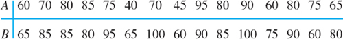
- Assuming normality, solve Prob. 6 by a suitable test from Sec. 25.4.
- In a clinical experiment, each of 10 patients were given two different sedatives A and B. The following table shows the effect (increase of sleeping time, measured in hours). Using the sign test, find out whether the difference is significant.
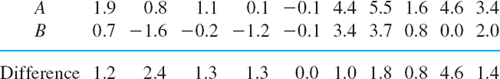
- Assuming that the populations corresponding to the samples in Prob. 8 are normal, apply a suitable test for the normal distribution.
- Test whether a thermostatic switch is properly set to 50°C against the alternative that its setting is too low. Use a sample of 9 values, 8 of which are less than 50°C and 1 is greater.
- How would you proceed in the sign test if the hypothesis is
 (any number) instead of
  ?
? - Test the hypothesis that, for a certain type of voltmeter, readings are independent of temperature T [°C] against the alternative that they tend to increase with T. Use a sample of values obtained by applying a constant voltage:
- Does the amount of fertilizer increase the yield of wheat X [kg/plot]? Use a sample of values ordered according to increasing amounts of fertilizer:

- Apply the test explained in Example 2 to the following data (x = diastolic blood pressure [mm Hg], y = weight of heart [in grams] of 10 patients who died of cerebral hemorrhage).

- Does an increase in temperature cause an increase of the yield of a chemical reaction from which the following sample was taken?
25.9 Regression. Fitting Straight Lines. Correlation
So far we were concerned with random experiments in which we observed a single quantity (random variable) and got samples whose values were single numbers. In this section we discuss experiments in which we observe or measure two quantities simultaneously, so that we get samples of pairs of values (x1, y1), (x2, y2), …, (xn, yn). Most applications involve one of two kinds of experiments, as follows.
- In regression analysis one of the two variables, call it x, can be regarded as an ordinary variable because we can measure it without substantial error or we can even give it values we want. x is called the independent variable, or sometimes the controlled variable because we can control it (set it at values we choose). The other variable, Y, is a random variable, and we are interested in the dependence of Y on x. Typical examples are the dependence of the blood pressure Y on the age x of a person or, as we shall now say, the regression of Y on x, the regression of the gain of weight Y of certain animals on the daily ration of food x, the regression of the heat conductivity Y of cork on the specific weight x of the cork, etc.
- In correlation analysis both quantities are random variables and we are interested in relations between them. Examples are the relation (one says “correlation”) between wear X and wear Y of the front tires of cars, between grades X and Y of students in mathematics and in physics, respectively, between the hardness X of steel plates in the center and the hardness Y near the edges of the plates, etc.
Regression Analysis
In regression analysis the dependence of Y on x is a dependence of the mean μ of Y on x, so that μ = μ(x) is a function in the ordinary sense. The curve of μ(x) is called the regression curve of Y on x.
In this section we discuss the simplest case, namely, that of a straight regression line

Then we may want to graph the sample values as n points in the xY-plane, fit a straight line through them, and use it for estimating μ(x) at values of x that interest us, so that we know what values of Y we can expect for those x. Fitting that line by eye would not be good because it would be subjective; that is, different persons’ results would come out differently, particularly if the points are scattered. So we need a mathematical method that gives a unique result depending only on the n points. A widely used procedure is the method of least squares by Gauss and Legendre. For our task we may formulate it as follows.
Least Squares Principle
The straight line should be fitted through the given points so that the sum of the squares of the distances of those points from the straight line is minimum, where the distance is measured in the vertical direction (the y-direction). (Formulas below.)
To get uniqueness of the straight line, we need some extra condition. To see this, take the sample (0, 1), (0, −1). Then all the lines y = k1x with any k1 satisfy the principle. (Can you see it?) The following assumption will imply uniqueness, as we shall find out.
General Assumption (A1)
The x-values x1, …, xn in our sample (x1, y1), …, (xn, yn) are not all equal.
From a given sample (x1, y1), …, (xn, yn) we shall now determine a straight line by least squares. We write the line as

and call it the sample regression line because it will be the counterpart of the population regression line (1).
Now a sample point (xj, yj) has the vertical distance (distance measured in the y-direction) from (2) given by

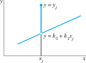
Fig. 543. Vertical distance of a point (xj, yj) from a straight line y = k0 + k1x
Hence the sum of the squares of these distances is
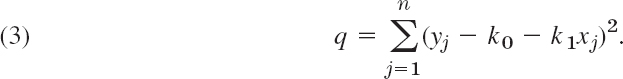
In the method of least squares we now have to determine k0 and k1 such that q is minimum. From calculus we know that a necessary condition for this is

We shall see that from this condition we obtain for the sample regression line the formula

Here ![]() and
and ![]() are the means of the x- and the y-values in our sample, that is,
are the means of the x- and the y-values in our sample, that is,
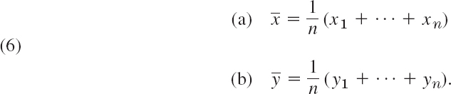
The slope k1 in (5) is called the regression coefficient of the sample and is given by

Here the “sample covariance” sxy is

and ![]() is given by
is given by

From (5) we see that the sample regression line passes through the point (![]() ), by which it is determined, together with the regression coefficient (7). We may call
), by which it is determined, together with the regression coefficient (7). We may call ![]() the variance of the x-values, but we should keep in mind that x is an ordinary variable, not a random variable.
the variance of the x-values, but we should keep in mind that x is an ordinary variable, not a random variable.
We shall soon also need

Derivation of (5) and (7). Differentiating (3) and using (4), we first obtain
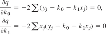
where we sum over j from 1 to n. We now divide by 2, write each of the two sums as three sums, and take the sums containing yj and xjyj over to the right. Then we get the “normal equations”

This is a linear system of two equations in the two unknowns k0 and k1. Its coefficient determinant is [see (9)]

and is not zero because of Assumption (A1). Hence the system has a unique solution. Dividing the first equation of (10) by n and using (6), we get ![]() . Together with y = k0 + k1x in (2) this gives (5). To get (7), we solve the system (10) by Cramer's rule (Sec. 7.6) or elimination, finding
. Together with y = k0 + k1x in (2) this gives (5). To get (7), we solve the system (10) by Cramer's rule (Sec. 7.6) or elimination, finding

This gives (7)–(9) and completes the derivation. [The equality of the two expressions in (8) and in (9) may be shown by the student].
The decrease of volume y[%] of leather for certain fixed values of high pressure x [atmospheres] was measured. The results are shown in the first two columns of Table 25.11. Find the regression line of y on x.
Solution. We see that n = 4 and obtain the values ![]() , and from (9) and (8)
, and from (9) and (8)
Table 25.11 Regression of the Decrease of Volume y [%] of Leather on the Pressure x [Atmospheres]


Hence k1 = 15,400/20,000,000 = 0.00077 from (7), and the regression line is
![]()
Note that y(0) = −0.64, which is physically meaningless, but typically indicates that a linear relation is merely an approximation valid on some restricted interval.
Confidence Intervals in Regression Analysis
If we want to get confidence intervals, we have to make assumptions about the distribution of Y (which we have not made so far; least squares is a “geometric principle,” nowhere involving probabilities!). We assume normality and independence in sampling:
Assumption (A2)
For each fixed x the random variable Y is normal with mean (1) , that is,
![]()
and variance σ2 independent of x.
Assumption (A3)
The n performances of the experiment by which we obtain a sample
![]()
are independent.
κ1 in (12) is called the regression coefficient of the population because it can be shown that, under Assumptions (A1)–(A3), the maximum likelihood estimate of κ1 is the sample regression coefficient k1 given by (11).
Under Assumptions (A1)–(A3), we may now obtain a confidence interval for κ1, as shown in Table 25.12.
Table 25.12 Determination of a Confidence Interval for κ1 in (1) under Assumptions (A1)–(A3)
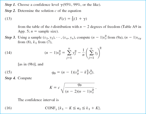
EXAMPLE 2 Confidence Interval for the Regression Coefficient
Using the sample in Table 25.11, determine a confidence interval for κ1 by the method in Table 25.12.
Solution. Step 1. We choose γ = 0.95.
Step 2. Equation (13) takes the form F(c) = 0.975, and Table A9 in App. 5 with n − 2 = 2 degrees of freedom gives c = 4.30.
Step 3. From Example 1 we have ![]() and k1 = 0.00077. From Table 25.11 we compute
and k1 = 0.00077. From Table 25.11 we compute
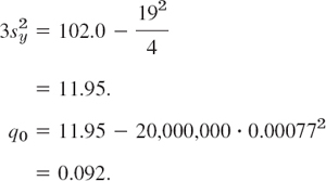
Step 4. We thus obtain

and
![]()
Correlation Analysis
We shall now give an introduction to the basic facts in correlation analysis; for proofs see Ref. [G2] or [G8] in App. 1.
Correlation analysis is concerned with the relation between X and Y in a two-dimensional random variable (X, Y) (Sec. 24.9). A sample consists of n ordered pairs of values (x1, y1), …, (xn, yn) as before. The interrelation between the x and y values in the sample is measured by the sample covariance sxy in (8) or by the sample correlation coefficient
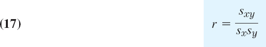
with sx and sy given in (9). Here r has the advantage that it does not change under a multiplication of the x and y values by a factor (in going from feet to inches, etc.).
THEOREM 1 Sample Correlation Coefficient
The sample correlation coefficient r satisfies − 1 ![]() r
r ![]() 1. In particular, r = ± 1 if and only if the sample values lie on a straight line. (See Fig. 544.)
1. In particular, r = ± 1 if and only if the sample values lie on a straight line. (See Fig. 544.)
The theoretical counterpart of r is the correlation coefficient ρ of X and Y,
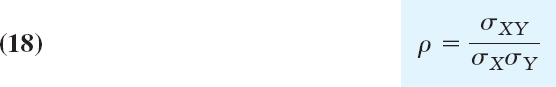

Fig. 544. Samples with various values of the correlation coefficient r
where ![]() (the means and variances of the marginal distributions of X and Y; see Sec. 24.9), and σXY is the covariance of X and Y given by (see Sec. 24.9)
(the means and variances of the marginal distributions of X and Y; see Sec. 24.9), and σXY is the covariance of X and Y given by (see Sec. 24.9)
![]()
The analog of Theorem 1 is
THEOREM 2 Correlation Coefficient
The correlation coefficient ρ satisfies −1 ![]() ρ
ρ ![]() 1. In particular, ρ = ±1 if and only if X and Y are linearly related, that is, Y = γX + ∂, X = γ*Y + ∂*.
1. In particular, ρ = ±1 if and only if X and Y are linearly related, that is, Y = γX + ∂, X = γ*Y + ∂*.
X and Y are called uncorrelated if ρ = 0.
THEOREM 3 Independence. Normal Distribution
- Independent X and Y (see Sec. 24.9) are uncorrelated.
- If (X, Y) is normal (see below), then uncorrelated X and Y are independent.
Here the two-dimensional normal distribution can be introduced by taking two independent standardized normal random variables X*, Y*, whose joint distribution thus has the density

(representing a surface of revolution over the x*y*-plane with a bell-shaped curve as cross section) and setting

This gives the general two-dimensional normal distribution with the density

where
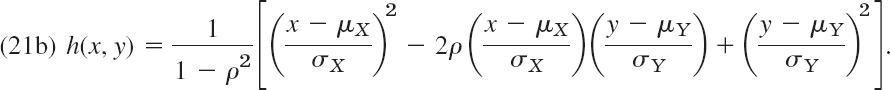
In Theorem 3(b), normality is important, as we can see from the following example.
EXAMPLE 3 Uncorrelated But Dependent Random Variables
If X assumes −1, 0, 1 with probability ![]() and Y = X2, then E(X) = 0 and in (3)
and Y = X2, then E(X) = 0 and in (3)
![]()
so that ρ = 0 and X and Y are uncorrelated. But they are certainly not independent since they are even functionally related.
Test for the Correlation Coefficient ρ
Table 25.13 shows a test for ρ in the case of the two-dimensional normal distribution. t is an observed value of a random variable that has a t-distribution with n − 2 degrees of freedom. This was shown by R. A. Fisher (Biometrika10 (1915), 507–521).
Table 25.13 Test of the Hypothesis ρ = 0 Against the Alternative ρ > 0 in the Case of the Two-Dimensional Normal Distribution
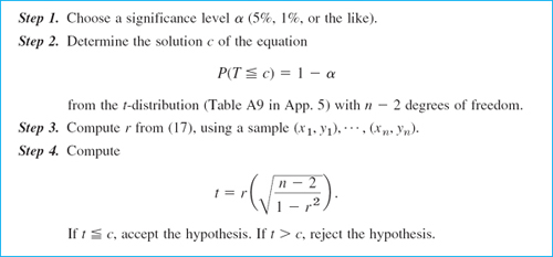
EXAMPLE 4 Test for the Correlation Coefficient ρ
Test the hypothesis ρ = 0 (independence of X and Y, because of Theorem 3) against the alternative ρ > 0, using the data in the lower left corner of Fig. 544, where r = 0.6 (manual soldering errors on 10 two-sided circuit boards done by 10 workers; x = front, y = back of the boards).
Solution. We choose α = 5%; thus 1 − α = 95%. Since n = 10, n − 2 = 8, the table gives c = 1.86. Also, ![]() . We reject the hypothesis and assert that there is a positive correlation. A worker making few (many) errors on the front side also tends to make few (many) errors on the reverse side of the board.
. We reject the hypothesis and assert that there is a positive correlation. A worker making few (many) errors on the front side also tends to make few (many) errors on the reverse side of the board.
1–10 SAMPLE REGRESSION LINE
Find and graph the sample regression line of y on x and the given data as points on the same axes. Show the details of your work.
- (0, 1.0), (2, 2.1), (4, 2.9), (6, 3.6), (8, 5.2)
- (−2, 3.5), (1, 2.6), (3, 1.3), (5, 0.4)
- x = Revolutions per minute, y = Power of a Diesel engine [hp]

- x = Deformation of a certain steel [mm], y = Brinell hardness [kg/mm2]
- x = Brinell hardness, y = Tensile strength [in 1000 psi (pounds per square inch)] of steel with 0.45% C tempered for 1 hour
- Abrasion of quenched and tempered steel S620. x = Sliding distance [km], y = Wear volume [mm2]

- Ohm's law (Sec. 2.9). x = Voltage [V], y = Current [A]. Also find the resistance R [Ω].
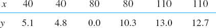
- Hooke's law (Sec. 2.4). x = Force [lb], y = Extension [in] of a spring. Also find the spring modulus.
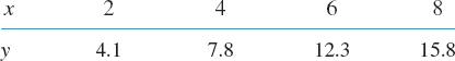
- Thermal conductivity of water. x = Temperature [°F], y = Conductivity[Btu/(hr · ft · °F)]. Also find y at room temperature 66°F.
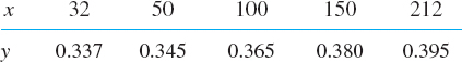
- Stopping distance of a car. x = Speed [mph]. y = Stopping distance [ft]. Also find y at 35 mph.

- CAS EXPERIMENT. Moving Data. Take a sample, for instance, that in Prob. 4, and investigate and graph the effect of changing y-values (a) for small x, (b) for large x, (c) in the middle of the sample.
12–15 CONFIDENCE INTERVALS
Find a 95% confidence interval for the regression coefficient κ1, assuming (A2) and (A3) hold and using the sample.
- 12. In Prob. 2
- 13. In Prob. 3
- 14. In Prob. 4
- 15. x = Humidity of air [%], y = Expansion of gelatin [%],
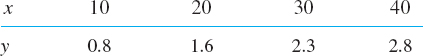
CHAPTER 25 REVIEW QUESTIONS AND PROBLEMS
- What is a sample? A population? Why do we sample in statistics?
- If we have several samples from the same population, do they have the same sample distribution function? The same mean and variance?
- Can we develop statistical methods without using probability theory? Apply the methods without using a sample?
- What is the idea of the maximum likelihood method? Why do we say “likelihood” rather than “probability”?
- Couldn't we make the error of interval estimation zero simply by choosing the confidence level 1?
- What is testing? Why do we test? What are the errors involved?
- When did we use the t-distribution? The F-distribution?
- What is the chi-square (X2) test? Give a sample example from memory.
- What are one-sided and two-sided tests? Give typical examples.
- How do we test in quality control? In acceptance sampling?
- What is the power of a test? What could you perhaps do when it is low?
- What is Gauss's least squares principle (which he found at age 18)?
- What is the difference between regression and correlation?
- Find the mean, variance, and standard derivation of the sample 21.0 21.6 19.9 19.6 15.6 20.6 22.1 22.2.
- Assuming normality, find the maximum likelihood estimates of mean and variance from the sample in Prob. 14.
- Determine a 95% confidence interval for the mean μ of a normal population with variance σ2 = 25, using a sample of size 500 with mean 22.
- Determine a 99% confidence interval for the mean of a normal population, using the sample 32, 33, 32, 34, 35, 29, 29, 27.
- Assuming normality, find a 95% confidence interval for the variance from the sample 145.3, 145.1, 145.4, 146.2.
- Using a sample of 10 values with mean 14.5 from a normal population with variance σ2 = 0.25, test the hypothesis μ0 = 15.0 against the alternative μ1 = 14.5 on the 5% level. Find the power.
- Three specimens of high-quality concrete had compressive strength 357, 359, 413 [kg/cm2], and for three specimens of ordinary concrete the values were 346, 358, 302. Test for equality of the population means,μ1 = μ2, against the alternative μ1 > μ2. Assume normality and equality of variance. Choose α = 5%.
- Assume the thickness X of washers to be normal with mean 2.75 mm and variance 0.00024 mm2. Set up a control chart for μ and graph the means of the five samples (2.74, 2.76), (2.74, 2.74), (2.79, 2.81), (2.78, 2.76), (2.71, 2.75) on the chart.
- The OC curve in acceptance sampling cannot have a strictly vertical portion. Why?
- Find the risks in the sampling plan with n = 6 and c = 0, assuming that the AQL is θ0 = 1% and the RQL is θ1 = 15%. How do the risks change if we increase n?
- Does a process of producing plastic rods of length
 meters need adjustment if in a sample, 2 rods have the exact length and 15 are shorter and 3 longer than 2 meters? (Use the sign test.)
 - Find the regression line of y on x for the data (x, y) = (0, 4), (2, 0), (4, −5), (6, −9), (8, −10).
SUMMARY OF CHAPTER 25
Mathematical Statistics
We recall from Chap. 24 that, with an experiment in which we observe some quantity (number of defectives, height of persons, etc.), there is associated a random variable X whose probability distribution is given by a distribution function
![]()
which for each x gives the probability that X assumes any value not exceeding x.
In statistics we take random samples x1, …, xn of size n by performing that experiment n times (Sec. 25.1) and draw conclusions from properties of samples about properties of the distribution of the corresponding X. We do this by calculating point estimates or confidence intervals or by performing a test for parameters (μ and σ2 in the normal distribution, p in the binomial distribution, etc.) or by a test for distribution functions.
A point estimate (Sec. 25.2) is an approximate value for a parameter in the distribution of X obtained from a sample. Notably, the sample mean (Sec. 25.1)

is an estimate of the mean μ of X, and the sample variance (Sec. 25.1)

is an estimate of the variance σ2 of X. Point estimation can be done by the basic maximum likelihood method (Sec. 25.2).
Confidence intervals (Sec. 25.3) are intervals θ1 ![]() θ
θ ![]() θ2 with endpoints calculated from a sample such that, with a high probability γ, we obtain an interval that contains the unknown true value of the parameter θ in the distribution of X. Here, γ is chosen at the beginning, usually 95% or 99%. We denote such an interval by CONFγ {θ1
θ2 with endpoints calculated from a sample such that, with a high probability γ, we obtain an interval that contains the unknown true value of the parameter θ in the distribution of X. Here, γ is chosen at the beginning, usually 95% or 99%. We denote such an interval by CONFγ {θ1 ![]() θ
θ ![]() θ2}.
θ2}.
In a test for a parameter we test a hypothesis θ = θ0 against an alternative θ = θ1 and then, on the basis of a sample, accept the hypothesis, or we reject it in favor of the alternative (Sec. 25.4). Like any conclusion about X from samples, this may involve errors leading to a false decision. There is a small probability α (which we can choose, 5% or 1%, for instance) that we reject a true hypothesis, and there is a probability β (which we can compute and decrease by taking larger samples) that we accept a false hypothesis. α is called the significance level and 1 − β the power of the test. Among many other engineering applications, testing is used in quality control (Sec. 25.5) and acceptance sampling (Sec. 25.6).
If not merely a parameter but the kind of distribution of X is unknown, we can use the chi-square test (Sec. 25.7) for testing the hypothesis that some function is the unknown distribution function of X. This is done by determining the discrepancy between F(x) and the distribution function ![]() of a given sample.
of a given sample.
“Distribution-free” or nonparametric tests are tests that apply to any distribution, since they are based on combinatorial ideas. These tests are usually very simple. Two of them are discussed in Sec. 25.8.
The last section deals with samples of pairs of values, which arise in an experiment when we simultaneously observe two quantities. In regression analysis, one of the quantities, x, is an ordinary variable and the other, Y, is a random variable whose mean μ depends on x, say, μ(x) = κ0 + κ1x. In correlation analysis the relation between X and Y in a two-dimensional random variable (X, Y) is investigated, notably in terms of the correlation coefficient ρ.
1JERZY NEYMAN (1894–1981), American statistician, developed the theory of confidence intervals (Annals of Mathematical Statistics 6 (1935), 111–116).
2Beginning around 1930, a systematic theory of tests was developed by NEYMAN (see Sec. 25.3) and EGON SHARPE PEARSON (1895–1980), English statistician, the son of Karl Pearson (see the footnote on p. 1086).
3This assumption of equality of variances can be tested, as shown in the next example. If the test shows that they differ significantly, choose two samples of the same size n1 =n2 = n (not too small, > 30, say), use the test in Example 2 together with the fact that (12) is an observed value of an approximately standardized normal random variable.
4After the pioneering work of the English statistician and biologist, KARL PEARSON (1857–1936), the founder of the English school of statistics, and WILLIAM SEALY GOSSET (1876–1937), who discovered the t-distribution (and published under the name “Student”), the English statistician Sir RONALD AYLMER FISHER (1890–1962), professor of eugenics in London (1933–1943) and professor of genetics in Cambridge, England (1943–1957) and Adelaide, Australia (1957–1962), had great influence on the further development of modern statistics.