
CHAPTER 2
Second-Order Linear ODEs

Many important applications in mechanical and electrical engineering, as shown in Secs. 2.4, 2.8, and 2.9, are modeled by linear ordinary differential equations (linear ODEs) of the second order. Their theory is representative of all linear ODEs as is seen when compared to linear ODEs of third and higher order, respectively. However, the solution formulas for second-order linear ODEs are simpler than those of higher order, so it is a natural progression to study ODEs of second order first in this chapter and then of higher order in Chap. 3.
Although ordinary differential equations (ODEs) can be grouped into linear and nonlinear ODEs, nonlinear ODEs are difficult to solve in contrast to linear ODEs for which many beautiful standard methods exist.
Chapter 2 includes the derivation of general and particular solutions, the latter in connection with initial value problems.
For those interested in solution methods for Legendre's, Bessel's, and the hypergeometric equations consult Chap. 5 and for Sturm–Liouville problems Chap. 11.
COMMENT. Numerics for second-order ODEs can be studied immediately after this chapter. See Sec. 21.3, which is independent of other sections in Chaps. 19–21.
Prerequisite: Chap. 1, in particular, Sec. 1.5.
Sections that may be omitted in a shorter course: 2.3, 2.9, 2.10.
References and Answers to Problems: App. 1 Part A, and App. 2.
2.1 Homogeneous Linear ODEs of Second Order
We have already considered first-order linear ODEs (Sec. 1.5) and shall now define and discuss linear ODEs of second order. These equations have important engineering applications, especially in connection with mechanical and electrical vibrations (Secs. 2.4, 2.8, 2.9) as well as in wave motion, heat conduction, and other parts of physics, as we shall see in Chap. 12.
A second-order ODE is called linear if it can be written

and nonlinear if it cannot be written in this form.
The distinctive feature of this equation is that it is linear in y and its derivatives, whereas the functions p, q, and r on the right may be any given functions of x. If the equation begins with, say, f(x)y″, then divide by f(x) to have the standard form (1) with y″ as the first term.
The definitions of homogeneous and nonhomogenous second-order linear ODEs are very similar to those of first-order ODEs discussed in Sec. 1.5. Indeed, if r(x) ≡ 0 (that is, r(x) = 0 for all x considered; read “r(x) is identically zero”), then (1) reduces to

and is called homogeneous. If r(x) ![]() 0, then (1) is called nonhomogeneous. This is similar to Sec. 1.5.
0, then (1) is called nonhomogeneous. This is similar to Sec. 1.5.
An example of a nonhomogeneous linear ODE is
![]()
and a homogeneous linear ODE is
![]()
Finally, an example of a nonlinear ODE is
![]()
The functions p and q in (1) and (2) are called the coefficients of the ODEs.
Solutions are defined similarly as for first-order ODEs in Chap. 1. A function
![]()
is called a solution of a (linear or nonlinear) second-order ODE on some open interval I if h is defined and twice differentiable throughout that interval and is such that the ODE becomes an identity if we replace the unknown y by h, the derivative y′ by h′, and the second derivative y″ by h″. Examples are given below.
Homogeneous Linear ODEs: Superposition Principle
Sections 2.1–2.6 will be devoted to homogeneous linear ODEs (2) and the remaining sections of the chapter to nonhomogeneous linear ODEs.
Linear ODEs have a rich solution structure. For the homogeneous equation the backbone of this structure is the superposition principle or linearity principle, which says that we can obtain further solutions from given ones by adding them or by multiplying them with any constants. Of course, this is a great advantage of homogeneous linear ODEs. Let us first discuss an example.
EXAMPLE 1 Homogeneous Linear ODEs: Superposition of Solutions
The functions y = cos x and y = sin x are solutions of the homogeneous linear ODE
![]()
for all x. We verify this by differentiation and substitution. We obtain (cos x)″ = −cos x hence
![]()
Similarly for y = sin x (verify!). We can go an important step further. We multiply cos x by any constant, for instance, 4.7, and sin x by, say, −2, and take the sum of the results, claiming that it is a solution. Indeed, differentiation and substitution gives
![]()
In this example we have obtained from y1 (= cos x) and y2 (= sin x) a function of the form
![]()
This is called a linear combination of y1 and y2. In terms of this concept we can now formulate the result suggested by our example, often called the superposition principle or linearity principle.
THEOREM 1 Fundamental Theorem for the Homogeneous Linear ODE (2)
For a homogeneous linear ODE (2), any linear combination of two solutions on an open interval I is again a solution of (2) on I. In particular, for such an equation, sums and constant multiples of solutions are again solutions.
PROOF
Let y1 and y2 be solutions of (2) on I. Then by substituting y = c1y1 + c2y2 and its derivatives into (2), and using the familiar rule ![]() , etc., we get
, etc., we get

since in the last line, (…) = 0 because y1 and y2 are solutions, by assumption. This shows that y is a solution of (2) on I.
CAUTION! Don't forget that this highly important theorem holds for homogeneous linear ODEs only but does not hold for nonhomogeneous linear or nonlinear ODEs, as the following two examples illustrate.
EXAMPLE 2 A Nonhomogeneous Linear ODE
Verify by substitution that the functions y = 1 + cos x and y = 1 + sin x are solutions of the nonhomogeneous linear ODE
![]()
but their sum is not a solution. Neither is, for instance, 2(1 + cos x) or 5(1 + sin x).
Verify by substitution that the functions y = x2 and y = 1 are solutions of the nonlinear ODE
![]()
but their sum is not a solution. Neither is −x2, so you cannot even multiply by −1!
Initial Value Problem. Basis. General Solution
Recall from Chap. 1 that for a first-order ODE, an initial value problem consists of the ODE and one initial condition y(x0) = y0. The initial condition is used to determine the arbitrary constant c in the general solution of the ODE. This results in a unique solution, as we need it in most applications. That solution is called a particular solution of the ODE. These ideas extend to second-order ODEs as follows.
For a second-order homogeneous linear ODE (2) an initial value problem consists of

These conditions prescribe given values K0 and K1 of the solution and its first derivative (the slope of its curve) at the same given x = x0 in the open interval considered.
The conditions (4) are used to determine the two arbitrary constants c1 and c2 in a general solution
of the ODE; here, y1 and y2 are suitable solutions of the ODE, with “suitable” to be explained after the next example. This results in a unique solution, passing through the point (x0, K0) with K1 as the tangent direction (the slope) at that point. That solution is called a particular solution of the ODE (2).
EXAMPLE 4 Initial Value Problem
Solve the initial value problem
![]()
Solution. Step 1. General solution. The functions cos x and sin x are solutions of the ODE (by Example 1), and we take
![]()

Fig. 29. Particular solution and initial tangent in Example 4
This will turn out to be a general solution as defined below.
Step 2. Particular solution. We need the derivative y′ = −c1 sin x + c2 cos x. From this and the initial values we obtain, since cos 0 = 1 and sin 0 = 0,
![]()
This gives as the solution of our initial value problem the particular solution
![]()
Figure 29 shows that at x = 0 it has the value 3.0 and the slope −0.5, so that its tangent intersects the x-axis at x = 3.0/0.5 = 6.0. (The scales on the axes differ!)
Observation. Our choice of y1 and y2 and was general enough to satisfy both initial conditions. Now let us take instead two proportional solutions y1 = cos x and y2 = k cos x, so that y1/y2 = 1/k = const. Then we can write y = c1y1 + c2y2 in the form
![]()
Hence we are no longer able to satisfy two initial conditions with only one arbitrary constant C. Consequently, in defining the concept of a general solution, we must exclude proportionality. And we see at the same time why the concept of a general solution is of importance in connection with initial value problems.
DEFINITION General Solution, Basis, Particular Solution
A general solution of an ODE (2) on an open interval I is a solution (5) in which and are solutions of (2) on I that are not proportional, and c1 and c2 are arbitrary constants. These y1, y2 are called a basis (or a fundamental system) of solutions of (2) on I.
A particular solution of (2) on I is obtained if we assign specific values to c1 and c2 in (5).
For the definition of an interval see Sec. 1.1. Furthermore, as usual, y1 and y2 are called proportional on I if for all x on I,
![]()
where k and l are numbers, zero or not. (Note that (a) implies (b) if and only if k ≠ 0).
Actually, we can reformulate our definition of a basis by using a concept of general importance. Namely, two functions y1 and y2 are called linearly independent on an interval I where they are defined if
![]()
And y1 and y2 are called linearly dependent on I if (7) also holds for some constants k1, k2 not both zero. Then, if k1 ≠ 0 or k2 ≠ 0, we can divide and see that y1 and y2 are proportional,
![]()
In contrast, in the case of linear independence these functions are not proportional because then we cannot divide in (7). This gives the following
DEFINITION Basis (Reformulated)
A basis of solutions of (2) on an open interval I is a pair of linearly independent solutions of (2) on I.
If the coefficients p and q of (2) are continuous on some open interval I, then (2) has a general solution. It yields the unique solution of any initial value problem (2), (4). It includes all solutions of (2) on I; hence (2) has no singular solutions (solutions not obtainable from of a general solution; see also Problem Set 1.1). All this will be shown in Sec. 2.6.
EXAMPLE 5 Basis, General Solution, Particular Solution
cos x and sin x in Example 4 form a basis of solutions of the ODE y″ + y = 0 for all x because their quotient is cot x ≠ const (or tan x ≠ const). Hence y = c1 cos x + c2 sin x is a general solution. The solution y = 3.0 cos x − 0.5 sin x of the initial value problem is a particular solution.
EXAMPLE 6 Basis, General Solution, Particular Solution
Verify by substitution that y1 = ex and y2 = e−x are solutions of the ODE y″ − y = 0. Then solve the initial value problem
![]()
Solution. (ex)″ − ex = 0 and (e−x)″ − e−x = 0 show that ex and e−x are solutions. They are not proportional, ex/e−x = e2x ≠ const. Hence ex, e−x form a basis for all x. We now write down the corresponding general solution and its derivative and equate their values at 0 to the given initial conditions,
![]()
By addition and subtraction, c1 = 2, c2 = 4, so that the answer is y = 2ex + 4e−x. This is the particular solution satisfying the two initial conditions.
Find a Basis if One Solution Is Known. Reduction of Order
It happens quite often that one solution can be found by inspection or in some other way. Then a second linearly independent solution can be obtained by solving a first-order ODE. This is called the method of reduction of order.1 We first show how this method works in an example and then in general.
EXAMPLE 7 Reduction of Order if a Solution Is Known. Basis
Find a basis of solutions of the ODE
![]()
Solution. Inspection shows that y1 = x is a solution because y′1 = 1 and y″1 = 0, so that the first term vanishes identically and the second and third terms cancel. The idea of the method is to substitute
![]()
into the ODE. This gives
![]()
ux and −xu cancel and we are left with the following ODE, which we divide by x, order, and simplify,
![]()
This ODE is of first order in ν = u′, namely, (x2 − x)ν′ + (x − 2)ν = 0. Separation of variables and integration gives
![]()
We need no constant of integration because we want to obtain a particular solution; similarly in the next integration. Taking exponents and integrating again, we obtain
![]()
Since y1 = x and y2 = x ln |x| + 1 are linearly independent (their quotient is not constant), we have obtained a basis of solutions, valid for all positive x.
In this example we applied reduction of order to a homogeneous linear ODE [see (2)]
![]()
Note that we now take the ODE in standard form, with y″, not f(x)y″—this is essential in applying our subsequent formulas. We assume a solution y1 of (2), on an open interval I, to be known and want to find a basis. For this we need a second linearly independent solution y2 of (2) on I. To get y2, we substitute
![]()
into (2). This gives
![]()
Collecting terms in u″, u′, and u, we have
![]()
Now comes the main point. Since y1 is a solution of (2), the expression in the last parentheses is zero. Hence u is gone, and we are left with an ODE in u′ and u″. We divide this remaining ODE by y1 and set u′ = U, u″ = U′,
![]()
This is the desired first-order ODE, the reduced ODE. Separation of variables and integration gives
![]()
By taking exponents we finally obtain
Here U = u′, so that u = ∫ U dx. Hence the desired second solution is
![]()
The quotient y2/y1 = u = ∫ U dx cannot be constant (since U > 0), so that y1 and y2 form a basis of solutions.
REDUCTION OF ORDER is important because it gives a simpler ODE. A general second-order ODE F(x, y, y′, y″) = 0, linear or not, can be reduced to first order if y does not occur explicitly (Prob. 1) or if x does not occur explicitly (Prob. 2) or if the ODE is homogeneous linear and we know a solution (see the text).
- Reduction. Show that F(x, y′, y″) = 0 can be reduced to first order in z = y′ (from which y follows by integration). Give two examples of your own.
- Reduction. Show that F(y, y′, y″) = 0 can be reduced to a first-order ODE with y as the independent variable and y″ = (dz/dy)z, where z = y′ derive this by the chain rule. Give two examples.
3–10 REDUCTION OF ORDER
Reduce to first order and solve, showing each step in detail.
- 3. y″ + y′ = 0
- 4. 2xy″ = 3y′
- 5. yy″ = 3y′2
- 6. xy″ + 2y′ + xy = 0, y1 = (cos x)/x
- 7. y″ + y′3 sin y = 0
- 8. y″ = 1 + y′2
- 9. x2y″ − 5xy′ + 9y = 0, y1 = x3
- 10. y″ + (1 + 1/y)y′2 = 0
11–14 APPLICATIONS OF REDUCIBLE ODEs
- 11. Curve. Find the curve through the origin in the xy-plane which satisfies y″ = 2y′ and whose tangent at the origin has slope 1.
- 12. Hanging cable. It can be shown that the curve y(x) of an inextensible flexible homogeneous cable hanging between two fixed points is obtained by solving
 , where the constant k depends on the weight. This curve is called catenary (from Latin catena = the chain). Find and graph y(x), assuming that k = 1 and those fixed points are (−1, 0) and (1, 0) in a vertical xy-plane.
 - 13. Motion. If, in the motion of a small body on a straight line, the sum of velocity and acceleration equals a positive constant, how will the distance y(t) depend on the initial velocity and position?
- 14. Motion. In a straight-line motion, let the velocity be the reciprocal of the acceleration. Find the distance y(t) for arbitrary initial position and velocity.
15–19 GENERAL SOLUTION. INITIAL VALUE PROBLEM (IVP)
(More in the next set.) (a) Verify that the given functions are linearly independent and form a basis of solutions of the given ODE. (b) Solve the IVP. Graph or sketch the solution.
- 15. 4y″ + 25y = 0, y(0) = 3.0, y′(0) = −2.5, cos 2.5x, sin 2.5x
- 16. y″ + 0.6y′ = 0.09y = 0, y(0) = 2.2, y′(0) = 0.14, e−0.3x, xe−0.3x
- 17. 4x2y″ − 3y = 0, y(1) = −3, y′(1) = 0, x3/2, x−1/2
- 18. x2y″ − xy′ + y = 0, y(1) = 4.3, y′(1) = 0.5, x, x ln x
- 19. y″ + 2y′ + 2y = 0, y(0) = 0, y′(0) = 15, e−x cos x, e−x sin x
- 20. CAS PROJECT. Linear Independence. Write a program for testing linear independence and dependence. Try it out on some of the problems in this and the next problem set and on examples of your own.
2.2 Homogeneous Linear ODEs with Constant Coefficients
We shall now consider second-order homogeneous linear ODEs whose coefficients a and b are constant,
These equations have important applications in mechanical and electrical vibrations, as we shall see in Secs. 2.4, 2.8, and 2.9.
To solve (1), we recall from Sec. 1.5 that the solution of the first-order linear ODE with a constant coefficient k
![]()
is an exponential function y = ce−kx. This gives us the idea to try as a solution of (1) the function
![]()
Substituting (2) and its derivatives
![]()
into our equation (1), we obtain
![]()
Hence if λ is a solution of the important characteristic equation (or auxiliary equation)

then the exponential function (2) is a solution of the ODE (1). Now from algebra we recall that the roots of this quadratic equation (3) are
![]()
(3) and (4) will be basic because our derivation shows that the functions
![]()
are solutions of (1). Verify this by substituting (5) into (1).
From algebra we further know that the quadratic equation (3) may have three kinds of roots, depending on the sign of the discriminant a2 − 4b, namely,

Case I. Two Distinct Real-Roots λ1 and λ2
In this case, a basis of solutions of (1) on any interval is
![]()
because y1 and y2 are defined (and real) for all x and their quotient is not constant. The corresponding general solution is

EXAMPLE 1 General Solution in the Case of Distinct Real Roots
We can now solve y″ − y = 0 in Example 6 of Sec. 2.1 systematically. The characteristic equation is λ2 − 1 = 0. Its roots are λ1 = 1 and λ = −1. Hence a basis of solutions is ex and e−x and gives the same general solution as before,
![]()
EXAMPLE 2 Initial Value Problem in the Case of Distinct Real Roots
Solve the initial value problem
![]()
Solution. Step 1. General solution. The characteristic equation is
![]()
Its roots are
![]()
so that we obtain the general solution
![]()
Step 2. Particular solution. Since y′ (x) = c1ex − 2c2e−2x, we obtain from the general solution and the initial conditions

Hence c1 = 1 and c2 = 3. This gives the answer y = ex + 3e−2x. Figure 30 shows that the curve begins at y = 4 with a negative slope (−5, but note that the axes have different scales!), in agreement with the initial conditions.
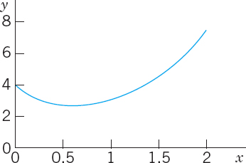
Fig. 30. Solution in Example 2
Case II. Real Double Root λ = −a/2
If the discriminant a2 − 4b is zero, we see directly from (4) that we get only one root, λ = λ1 = λ2 = −a/2, hence only one solution,
![]()
To obtain a second independent solution y2 (needed for a basis), we use the method of reduction of order discussed in the last section, setting y2 = uy1. Substituting this and its derivatives y′2 = u′ y1 + uy′1 and y″2 into (1), we first have
![]()
Collecting terms in u″, u′, and u, as in the last section, we obtain
![]()
The expression in the last parentheses is zero, since y1 is a solution of (1). The expression in the first parentheses is zero, too, since
![]()
We are thus left with y″y1 = 0. Hence u″ = 0. By two integrations, u = c1x + c2. To get a second independent solution y2 = uy1, we can simply choose c1, c2 = 0 and take u = x. Then y2 = xy1. Since these solutions are not proportional, they form a basis. Hence in the case of a double root of (3) a basis of solutions of (1) on any interval is
![]()
The corresponding general solution is

WARNING! If λ is a simple root of (4), then (c1 + c2x)eλx with is c2 ≠ 0 is not a solution of (1).
EXAMPLE 3 General Solution in the Case of a Double Root
The characteristic equation of the ODE y″ + 6y′ + 9y = 0 is λ2 + 6λ + 9 = (λ + 3)2 = 0. It has the double root λ = −3. Hence a basis is e−3x and xe−3x. The corresponding general solution is y = (c1 + c2x)e−3x.
EXAMPLE 4 Initial Value Problem in the Case of a Double Root
Solve the initial value problem
![]()
Solution. The characteristic equation is λ2 + λ + 0.25 = (λ + 0.5)2 = 0. It has the double root λ = −0.5. This gives the general solution
![]()
We need its derivative
![]()
From this and the initial conditions we obtain
![]()
The particular solution of the initial value problem is y = (3 − 2x)e−0.5x. See Fig. 31.

Fig. 31. Solution in Example 4
Case III. Complex Roots 
This case occurs if the discriminant a2 − 4b of the characteristic equation (3) is negative. In this case, the roots of (3) are the complex ![]() that give the complex solutions of the ODE (1). However, we will show that we can obtain a basis of real solutions
that give the complex solutions of the ODE (1). However, we will show that we can obtain a basis of real solutions
![]()
where ![]() . It can be verified by substitution that these are solutions in the present case. We shall derive them systematically after the two examples by using the complex exponential function. They form a basis on any interval since their quotient is not constant. Hence a real general solution in Case III is
. It can be verified by substitution that these are solutions in the present case. We shall derive them systematically after the two examples by using the complex exponential function. They form a basis on any interval since their quotient is not constant. Hence a real general solution in Case III is

EXAMPLE 5 Complex Roots. Initial Value Problem
Solve the initial value problem
![]()
Solution. Step 1. General solution. The characteristic equation is λ2 + 0.4λ + 9.04 = 0. It has the roots −0.2 ± 3i. Hence ω = 3, and a general solution (9) is
![]()
Step 2. Particular solution. The first initial condition gives y(0) = A = 0. The remaining expression is y = Be−0.2x sin 3x. We need the derivative (chain rule!)
![]()
From this and the second initial condition we obtain y′(0) = 3B = 3. Hence B = 1. Our solution is
![]()
Figure 32 shows y and the curves of e−0.2x and −e−0.2x (dashed), between which the curve of y oscillates. Such “damped vibrations” (with x = t being time) have important mechanical and electrical applications, as we shall soon see (in Sec. 2.4).

Fig. 32. Solution in Example 5
A general solution of the ODE
![]()
is
![]()
Summary of Cases I–III

It is very interesting that in applications to mechanical systems or electrical circuits, these three cases correspond to three different forms of motion or flows of current, respectively. We shall discuss this basic relation between theory and practice in detail in Sec. 2.4 (and again in Sec. 2.8).
Derivation in Case III. Complex Exponential Function
If verification of the solutions in (8) satisfies you, skip the systematic derivation of these real solutions from the complex solutions by means of the complex exponential function ez of a complex variable z = r + it. We write r + it, not x + iy because x and y occur in the ODE. The definition of ez in terms of the real functions er, cos t, and sin t is
![]()
This is motivated as follows. For real z = r, hence t = 0, cos 0 = 1, sin 0 = 0, we get the real exponential function er. It can be shown that ![]() , just as in real. (Proof in Sec. 13.5.) Finally, if we use the Maclaurin series of ez with z = it as well as i2 = −1, i3 = −i, i4 = 1, etc., and reorder the terms as shown (this is permissible, as can be proved), we obtain the series
, just as in real. (Proof in Sec. 13.5.) Finally, if we use the Maclaurin series of ez with z = it as well as i2 = −1, i3 = −i, i4 = 1, etc., and reorder the terms as shown (this is permissible, as can be proved), we obtain the series

(Look up these real series in your calculus book if necessary.) We see that we have obtained the formula

called the Euler formula. Multiplication by er gives (10).
For later use we note that e−it = cos (−t) + i sin (−t) = cos t − i sin t, so that by addition and subtraction of this and (11),

After these comments on the definition (10), let us now turn to Case III.
In Case III the radicand a2 − 4b in (4) is negative. Hence 4b − a2 is positive and, using ![]() , we obtain in (4)
, we obtain in (4)
![]()
with ω defined as in (8). Hence in (4),
![]()
Using (10) with ![]() and t = ωx, we thus obtain
and t = ωx, we thus obtain

We now add these two lines and multiply the result by ![]() . This gives y1 as in (8). Then we subtract the second line from the first and multiply the result by 1/(2i). This gives y2 as in (8). These results obtained by addition and multiplication by constants are again solutions, as follows from the superposition principle in Sec. 2.1. This concludes the derivation of these real solutions in Case III.
. This gives y1 as in (8). Then we subtract the second line from the first and multiply the result by 1/(2i). This gives y2 as in (8). These results obtained by addition and multiplication by constants are again solutions, as follows from the superposition principle in Sec. 2.1. This concludes the derivation of these real solutions in Case III.
1–15 GENERAL SOLUTION
Find a general solution. Check your answer by substitution. ODEs of this kind have important applications to be discussed in Secs. 2.4, 2.7, and 2.9.
- 4y″ − 25y = 0
- y″ + 36y = 0
- y″ + 6y′ + 8.96y = 0
- y″ + 4y′ + (π2 + 4)y = 0
- y″ + 2πy′ + π2y = 0
- 10y″ − 32y′ + 25.6y = 0
- y″ + 4.5y′ = 0
- y″ + y′ + 3.25y = 0
- y″ + 1.8y′ − 2.08y = 0
- 100y″ + 240y′ + (196π2 + 144)y = 0
- 4y″ − 4y′ − 3y = 0
- y″ + 9y′ + 20y = 0
- 9y″ − 30y′ + 25y = 0
- y″ + 2k2y′ + k4y = 0
- y″ + 0.54y′ + (0.0729 + π)y = 0
16–20 FIND AN ODE
y″ + ay′ + by = 0 for the given basis.
- 16. e2.6x, e−4.3x
- 17.

- 18. cos 2πx, sin 2πx
- 19. 3(−2+i)x, e(−2−i)x
- 20. e−3.1x cos 2.1x, e−3.1x sin 2.1 x
21–30 INITIAL VALUES PROBLEMS
Solve the IVP. Check that your answer satisfies the ODE as well as the initial conditions. Show the details of your work.
- 21. y″ + 25y = 0, y(0) = 4.6, y′(0) = −1.2
- 22. The ODE in Prob. 4,

- 23. y″ + y′ − 6y = 0, y(0) = 10, y′(0) = 0
- 24. 4y″ − 4y′ − 3y = 0, y(−2) = e, y′(−2) = −e/2
- 25. y″ − y = 0, y(0) = 2, y′(0) = −2
- 26. y″ − k2y = 0 (k ≠ 0), y(0) = 1, y′(0) = 1
- 27. The ODE in Prob. 5,
y(0) = 4.5, y′(0) = −4.5π − 1 = 13.137
- 28. 8y″ − 2y′ − y = 0, y(0) = − 0.2, y′(0) = −0.325
- 29. The ODE in Prob. 15, y(0) = 0, y′(0) = 1
- 30. 9y″ − 30y′ + 25y = 0, y(0) = 3.3, y′(0) = 10.0
31–36 LINEAR INDEPENDENCE is of basic importance, in this chapter, in connection with general solutions, as explained in the text. Are the following functions linearly independent on the given interval? Show the details of your work.
- 31. ekx, xekx, any interval
- 32. eax, e−ax, x > 0
- 33. x2, x2 ln x, x > 1
- 34. ln x, ln (x3), x > 1
- 35. sin 2x, cos x sin x, x < 0
- 36.

- 37. Instability. Solve y″ − y = 0 for the initial conditions y(0) = 1, y′(0) = −1. Then change the initial conditions to y(0) = 1.001, y′(0) = −0.999 and explain why this small change of 0.001 at t = 0 causes a large change later, e.g., 22 at t = 10. This is instability: a small initial difference in setting a quantity (a current, for instance) becomes larger and larger with time t. This is undesirable.
- 38. TEAM PROJECT. General Properties of Solutions (a) Coefficient formulas. Show how a and b in (1) can be expressed in terms of λ1 and λ2. Explain how these formulas can be used in constructing equations for given bases.
(b) Root zero. Solve y″ + 4y′ = 0 (i) by the present method, and (ii) by reduction to first order. Can you explain why the result must be the same in both cases? Can you do the same for a general ODE y″ + ay′ = 0?
(c) Double root. Verify directly that xeλx with λ = −a/2 is a solution of (1) in the case of a double root. Verify and explain why y = e−2x is a solution of y″ − y′ − 6y = 0 but xe−2x is not.
(d) Limits. Double roots should be limiting cases of distinct roots λ1, λ2 as, say, λ2 → λ1. Experiment with this idea. (Remember l'Hôpital's rule from calculus.) Can you arrive at
 ? Give it a try.
2.3 Differential Operators. Optional
This short section can be omitted without interrupting the flow of ideas. It will not be used subsequently, except for the notations Dy, D2y etc. to stand for y′, y″, etc.
Operational calculus means the technique and application of operators. Here, an operator is a transformation that transforms a function into another function. Hence differential calculus involves an operator, the differential operator D, which transforms a (differentiable) function into its derivative. In operator notation we write ![]() and
and
Similarly, for the higher derivatives we write D2y = D(Dy) = y″, and so on. For example, D sin = cos, D2 sin = −sin, etc.
For a homogeneous linear ODE y″ + ay′ + by = 0 with constant coefficients we can now introduce the second-order differential operator
![]()
where I is the identity operator defined by Iy = y. Then we can write that ODE as
![]()
P suggests “polynomial.” L is a linear operator. By definition this means that if Ly and Lw exist (this is the case if y and w are twice differentiable), then L(cy + kw) exists for any constants c and k, and
![]()
Let us show that from (2) we reach agreement with the results in Sec. 2.2. Since (Deλ)(x) = λeλx and (D2eλ)(x) = λ2eλx, we obtain
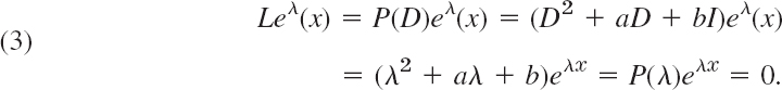
This confirms our result of Sec. 2.2 that eλx is a solution of the ODE (2) if and only if λ is a solution of the characteristic equation P(λ) = 0.
P(λ) is a polynomial in the usual sense of algebra. If we replace λ by the operator D, we obtain the “operator polynomial” P(D). The point of this operational calculus is that P(D) can be treated just like an algebraic quantity. In particular, we can factor it.
EXAMPLE 1 Factorization, Solution of an ODE
Factor P(D) = D2 − 3D − 40I and solve P(D)y = 0.
Solution. D2 − 3D − 40I = (D − 8I)(D + 5I) because I2 = I. Now (D − 8I)y = y′ − 8y = 0 has the solution y1 = e8x. Similarly, the solution of (D + 5I)y = 0 is y2 =e−5x. This is a basis of P(D)y = 0 on any interval. From the factorization we obtain the ODE, as expected,
![]()
Verify that this agrees with the result of our method in Sec. 2.2. This is not unexpected because we factored in the same way as the characteristic polynomial P(λ) = λ2 − 3λ − 40.
It was essential that L in (2) had constant coefficients. Extension of operator methods to variable-coefficient ODEs is more difficult and will not be considered here.
If operational methods were limited to the simple situations illustrated in this section, it would perhaps not be worth mentioning. Actually, the power of the operator approach appears in more complicated engineering problems, as we shall see in Chap. 6.
1–5 APPLICATION OF DIFFERENTIAL OPERATORS
Apply the given operator to the given functions. Show all steps in detail.
- D2 + 2D; cosh 2x, e−x + e2x, cos x
- D − 3I; 3x2 + 3x, 3e3x, cos 4x − sin 4x
- (D − 2I)2; e2x, xe2x, e−2x
- D + 6I)2; 6x + sin 6x, xe−6x
- (D − 2I)(D + 3I); e2x, xe2x, e−3x
6–12 GENERAL SOLUTION
Factor as in the text and solve.
- 6. (D2 + 4.00D + 3.36I)y = 0
- 7. (4D2 − I)y = 0
- 8. (D2 + 3I)y = 0
- 9. (D2 − 4.30D + 4.41I)y = 0
- 10. (D2 + 4.80D + 5.76I)y = 0
- 11. (D2 − 4.00D + 3.84I)y = 0
- 12. (D2 + 3.0D + 2.51I)y = 0
- 13. Linear operator. Illustrate the linearity of L in (2) by taking c = 4, k = −6, y = e2x, and w = cos 2x. Prove that L is linear.
- 14. Double root. If D2 + aD + bI has distinct roots μ and λ, show that a particular solution is y = (eμx − eλx)/(μ − λ). Obtain from this a solution xeλx by letting μ → λ and applying l'Hôpital's rule.
- 15. Definition of linearity. Show that the definition of linearity in the text is equivalent to the following. If L[y] and L[w] exist, then L[y + w] exists and L[cy] and L[kw] exist for all constants c and k, and L[y + w] = L[y] + L[w] as well as L[cy] = cL[y] and L[kw] = kL[w].
2.4 Modeling of Free Oscillations of a Mass–Spring System
Linear ODEs with constant coefficients have important applications in mechanics, as we show in this section as well as in Sec. 2.8, and in electrical circuits as we show in Sec. 2.9. In this section we model and solve a basic mechanical system consisting of a mass on an elastic spring (a so-called “mass–spring system,” Fig. 33), which moves up and down.
Setting Up the Model
We take an ordinary coil spring that resists extension as well as compression. We suspend it vertically from a fixed support and attach a body at its lower end, for instance, an iron ball, as shown in Fig. 33. We let y = 0 denote the position of the ball when the system is at rest (Fig. 33b). Furthermore, we choose the downward direction as positive, thus regarding downward forces as positive and upward forces as negative.

Fig. 33. Mechanical mass–spring system
We now let the ball move, as follows. We pull it down by an amount y > 0 (Fig. 33c). This causes a spring force

proportional to the stretch y, with k (>0) called the spring constant. The minus sign indicates that F1 points upward, against the displacement. It is a restoring force: It wants to restore the system, that is, to pull it back to y = 0. Stiff springs have large k.
Note that an additional force −F0 is present in the spring, caused by stretching it in fastening the ball, but F0 has no effect on the motion because it is in equilibrium with the weight W of the ball, −F0 = W = mg, where g = 980 cm/sec2 = 9.8 m/sec2 = 32.17 ft/sec2 is the constant of gravity at the Earth's surface (not to be confused with the universal gravitational constant G = gR2/M = 6.67 · 10−11 nt m2/kg2, which we shall not need; here R = 6.37 · 106 m and M = 5.98 · 1024 kg are the Earth's radius and mass, respectively).
The motion of our mass–spring system is determined by Newton's second law

where y″ = d2y/dt2 and “Force” is the resultant of all the forces acting on the ball. (For systems of units, see the inside of the front cover.)
ODE of the Undamped System
Every system has damping. Otherwise it would keep moving forever. But if the damping is small and the motion of the system is considered over a relatively short time, we may disregard damping. Then Newton's law with F = −F1 gives the model my″ = −F1 = −ky; thus

This is a homogeneous linear ODE with constant coefficients. A general solution is obtained as in Sec. 2.2, namely (see Example 6 in Sec. 2.2)

This motion is called a harmonic oscillation (Fig. 34). Its frequency is f = ω0/2π Hertz3 (= cycles/sec) because and in (4) have the period 2π/ω0. The frequency f is called the natural frequency of the system. (We write ω0 to reserve ω for Sec. 2.8.)

Fig. 34. Typical harmonic oscillations (4) and (4*) with the same y(0) = A and different initial velocities y′(0) = ω0B, positive ![]() , zero
, zero ![]() , negative
, negative ![]()
An alternative representation of (4), which shows the physical characteristics of amplitude and phase shift of (4), is

with ![]() and phase angle δ, where tan δ = B/A. This follows from the addition formula (6) in App. 3.1.
and phase angle δ, where tan δ = B/A. This follows from the addition formula (6) in App. 3.1.
EXAMPLE 1 Harmonic Oscillation of an Undamped Mass–Spring System
If a mass–spring system with an iron ball of weight W = 98 nt (about 22 lb) can be regarded as undamped, and the spring is such that the ball stretches it 1.09 m (about 43 in.), how many cycles per minute will the system execute? What will its motion be if we pull the ball down from rest by 16 cm (about 6 in.) and let it start with zero initial velocity?
Solution. Hooke's law (1) with W as the force and 1.09 meter as the stretch gives W = 1.09k; thus k = W/1.09 = 98/1.09 = 90[kg/sec2] = 90 [nt>meter]. The mass is m = W/g = 98/9.8 = 10 [kg]. This gives the frequency ![]() .
.
From (4) and the initial conditions, y(0) = A = 0.16 [meter] and y′(0) = ω0B = 0. Hence the motion is
![]()
If you have a chance of experimenting with a mass–spring system, don't miss it. You will be surprised about the good agreement between theory and experiment, usually within a fraction of one percent if you measure carefully.

Fig. 35. Harmonic oscillation in Example 1
ODE of the Damped System
To our model my″ = −ky we now add a damping force
![]()
obtaining my″ = −ky − cy′; thus the ODE of the damped mass–spring system is

Physically this can be done by connecting the ball to a dashpot; see Fig. 36. We assume this damping force to be proportional to the velocity y′ = dy/dt. This is generally a good approximation for small velocities.

The constant c is called the damping constant. Let us show that c is positive. Indeed, the damping force F2 = −cy′ acts against the motion; hence for a downward motion we have y′ > 0 which for positive c makes F negative (an upward force), as it should be. Similarly, for an upward motion we have y′ < 0 which, for c > 0 makes F2 positive (a downward force).
The ODE (5) is homogeneous linear and has constant coefficients. Hence we can solve it by the method in Sec. 2.2. The characteristic equation is (divide (5) by m)
![]()
By the usual formula for the roots of a quadratic equation we obtain, as in Sec. 2.2,

It is now interesting that depending on the amount of damping present—whether a lot of damping, a medium amount of damping or little damping—three types of motions occur, respectively:

They correspond to the three Cases I, II, III in Sec. 2.2.
Discussion of the Three Cases
Case I. Overdamping
If the damping constant c is so large that c2 > 4mk, then λ1 and λ2 are distinct real roots. In this case the corresponding general solution of (5) is

We see that in this case, damping takes out energy so quickly that the body does not oscillate. For t > 0 both exponents in (7) are negative because α > 0, β > 0, and β2 = α2 − k/m < α2. Hence both terms in (7) approach zero as t → ∞. Practically speaking, after a sufficiently long time the mass will be at rest at the static equilibrium position (y = 0). Figure 37 shows (7) for some typical initial conditions.

Fig. 37. Typical motions (7) in the overdamped case
(a) Positive initial displacement
(b) Negative initial displacement
Case II. Critical Damping
Critical damping is the border case between nonoscillatory motions (Case I) and oscillations (Case III). It occurs if the characteristic equation has a double root, that is, if c2 = 4mk, so that β = 0, λ1 = λ2 = −α. Then the corresponding general solution of (5) is

This solution can pass through the equilibrium position y = 0 at most once because e−αt is never zero and c1 + c2t can have at most one positive zero. If both c1 and c2 are positive (or both negative), it has no positive zero, so that y does not pass through 0 at all. Figure 38 shows typical forms of (8). Note that they look almost like those in the previous figure.

Fig. 38. Critical damping [see (8)]
Case III. Underdamping
This is the most interesting case. It occurs if the damping constant c is so small that c2 < 4mk. Then β in (6) is no longer real but pure imaginary, say,

(We now write ω* to reserve ω for driving and electromotive forces in Secs. 2.8 and 2.9.) The roots of the characteristic equation are now complex conjugates,
![]()
with α = c/(2m), as given in (6). Hence the corresponding general solution is

where C2 = A2 + B2 and tan δ = B/A, as in (4*).
This represents damped oscillations. Their curve lies between the dashed curves y = Ce−αt and y = −Ce−αt in Fig. 39, touching them when ω*t − δ is an integer multiple of π because these are the points at which cos (ω*t − δ) equals 1 or −1.
The frequency is ω*/(2π) Hz (hertz, cycles/sec). From (9) we see that the smaller c (>0) is, the larger is ω* and the more rapid the oscillations become. If c approaches 0, then ω* approaches ![]() , giving the harmonic oscillation (4), whose frequency ω0/(2π) is the natural frequency of the system.
, giving the harmonic oscillation (4), whose frequency ω0/(2π) is the natural frequency of the system.

Fig. 39. Damped oscillation in Case III [see (10)]
EXAMPLE 2 The Three Cases of Damped Motion
How does the motion in Example 1 change if we change the damping constant c from one to another of the following three values, with y(0) = 0.16 and y′(0) = 0 as before?
![]()
Solution. It is interesting to see how the behavior of the system changes due to the effect of the damping, which takes energy from the system, so that the oscillations decrease in amplitude (Case III) or even disappear (Cases II and I).
(I) With m = 10 and k = 90, as in Example 1, the model is the initial value problem
![]()
The characteristic equation is 10λ2 + 100λ + 90 = 10(λ + 9)(λ + 1) = 0. It has the roots −9 and −1. This gives the general solution
![]()
The initial conditions give c1 + c2 = 0.16, −9c1 − c2 = 0. The solution is c1 = −0.02, c2 = 0.18. Hence in the overdamped case the solution is
![]()
It approaches 0 as t → ∞. The approach is rapid; after a few seconds the solution is practically 0, that is, the iron ball is at rest.
(II) The model is as before, with c = 60 instead of 100. The characteristic equation now has the form 10λ2 + 60λ + 90 = 10(λ + 3)2 = 0. It has the double root −3. Hence the corresponding general solution is
![]()
The initial conditions give y(0) = c1 = 0.16, y′(0) = c2 − 3c1 = 0, c2 = 0.48. Hence in the critical case the solution is
![]()
It is always positive and decreases to 0 in a monotone fashion.
(III) The model now is 10y″ + 10y′ + 90y = 0. Since c = 10 is smaller than the critical c, we shall get oscillations. The characteristic equation is ![]() . It has the complex roots [see (4) in Sec. 2.2 with a = 1 and b = 9]
. It has the complex roots [see (4) in Sec. 2.2 with a = 1 and b = 9]
![]()
This gives the general solution
![]()
Thus y(0) = A = 0.16. We also need the derivative
![]()
Hence y′(0) = −0.5A + 2.96B = 0, B = 0.5A/2.96 = 0.027. This gives the solution
![]()
We see that these damped oscillations have a smaller frequency than the harmonic oscillations in Example 1 by about 1% (since 2.96 is smaller than 3.00 by about 1%). Their amplitude goes to zero. See Fig. 40.

Fig. 40. The three solutions in Example 2
This section concerned free motions of mass–spring systems. Their models are homogeneous linear ODEs. Nonhomogeneous linear ODEs will arise as models of forced motions, that is, motions under the influence of a “driving force.” We shall study them in Sec. 2.8, after we have learned how to solve those ODEs.
1–10 HARMONIC OSCILLATIONS (UNDAMPED MOTION)
- Initial value problem. Find the harmonic motion (4) that starts from y0 with initial velocity ν0. Graph or sketch the solutions for ω0 = π, y0 = 1, and various ν0 of your choice on common axes. At what t-values do all these curves intersect? Why?
- Frequency. If a weight of 20 nt (about 4.5 lb) stretches a certain spring by 2 cm, what will the frequency of the corresponding harmonic oscillation be? The period?
- Frequency. How does the frequency of the harmonic oscillation change if we (i) double the mass, (ii) take a spring of twice the modulus? First find qualitative answers by physics, then look at formulas.
- Initial velocity. Could you make a harmonic oscillation move faster by giving the body a greater initial push?
- Springs in parallel. What are the frequencies of vibration of a body of mass m = 5 kg (i) on a spring of modulus k1 = 20 nt/m, (ii) on a spring of modulus k2 = 45 nt/m, (iii) on the two springs in parallel? See Fig. 41.

- Spring in series. If a body hangs on a spring s1 of modulus k1 = 8, which in turn hangs on a spring s2 of modulus k2 = 12, what is the modulus k of this combination of springs?
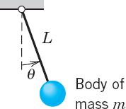
- Pendulum. Find the frequency of oscillation of a pendulum of length L (Fig. 42), neglecting air resistance and the weight of the rod, and assuming θ to be so small that sin θ practically equals θ.
- Archimedian principle. This principle states that the buoyancy force equals the weight of the water displaced by the body (partly or totally submerged). The cylindrical buoy of diameter 60 cm in Fig. 43 is floating in water with its axis vertical. When depressed downward in the water and released, it vibrates with period 2 sec. What is its weight?

- Vibration of water in a tube. If 1 liter of water (about 1.06 US quart) is vibrating up and down under the influence of gravitation in a U-shaped tube of diameter 2 cm (Fig. 44), what is the frequency? Neglect friction. First guess.

- TEAM PROJECT. Harmonic Motions of Similar Models. The unifying power of mathematical methods results to a large extent from the fact that different physical (or other) systems may have the same or very similar models. Illustrate this for the following three systems
(a) Pendulum clock. A clock has a 1-meter pendulum. The clock ticks once for each time the pendulum completes a full swing, returning to its original position. How many times a minute does the clock tick?
(b) Flat spring (Fig. 45). The harmonic oscillations of a flat spring with a body attached at one end and horizontally clamped at the other are also governed by (3). Find its motions, assuming that the body weighs 8 nt (about 1.8 lb), the system has its static equilibrium 1 cm below the horizontal line, and we let it start from this position with initial velocity 10 cm/sec.

(c) Torsional vibrations (Fig. 46). Undamped torsional vibrations (rotations back and forth) of a wheel attached to an elastic thin rod or wire are governed by the equation I0θ″ + Kθ = 0, where θ is the angle measured from the state of equilibrium. Solve this equation for K/I0 = 13.69 sec−2, initial angle 30° (= 0.5235 rad) and initial angular velocity 20° sec−1 (= 0.349 rad · sec−1).

11–20 DAMPED MOTION
- 11. Overdamping. Show that for (7) to satisfy initial conditions y(0) = y0 and ν(0) = ν0 we must have c1 = [(1 + α/β)y0 + ν0/β]/2 and c2 = [(1 − α/β)y0 − ν0/β]/2.
- 12. Overdamping. Show that in the overdamped case, the body can pass through y = 0 at most once (Fig. 37).
- 13. Initial value problem. Find the critical motion (8) that starts from with initial velocity ν0. Graph solution curves for α = 1, y0 = 1 and several ν0 such that (i) the curve does not intersect the t- axis, (ii) it intersects it at t = 1, 2, …, 5, respectively.
- 14. Shock absorber. What is the smallest value of the damping constant of a shock absorber in the suspension of a wheel of a car (consisting of a spring and an absorber) that will provide (theoretically) an oscillation-free ride if the mass of the car is 2000 kg and the spring constant equals 4500 kg/sec2?
- 15. Frequency. Find an approximation formula for ω* in terms of ω0 by applying the binomial theorem in (9) and retaining only the first two terms. How good is the approximation in Example 2, III?
- 16. Maxima. Show that the maxima of an underdamped motion occur at equidistant t- values and find the distance.
- 17. Underdamping. Determine the values of t corresponding to the maxima and minima of the oscillation y(t) = e−t sin t. Check your result by graphing y(t).
- 18. Logarithmic decrement. Show that the ratio of two consecutive maximum amplitudes of a damped oscillation (10) is constant, and the natural logarithm of this ratio called the logarithmic decrement, equals Δ = 2πα/ω*. Find Δ for the solutions of y″ + 2y′ + 5y = 0.
- 19. Damping constant. Consider an underdamped motion of a body of mass m = 0.5. If the time between two consecutive maxima is 3 sec and the maximum amplitude decreases to
 its initial value after 10 cycles, what is the damping constant of the system?
 - 20. CAS PROJECT. Transition Between Cases I, II, III. Study this transition in terms of graphs of typical solutions. (Cf. Fig. 47.)
(a) Avoiding unnecessary generality is part of good modeling. Show that the initial value problems (A) and (B),

(B) the same with different c and y′(0) = −2 (instead of 0), will give practically as much information as a problem with other m, k, y(0), y′(0).
(b) Consider (A). Choose suitable values of c, perhaps better ones than in Fig. 47, for the transition from Case III to II and I. Guess c for the curves in the figure.
(c) Time to go to rest. Theoretically, this time is infinite (why?). Practically, the system is at rest when its motion has become very small, say, less than 0.1% of the initial displacement (this choice being up to us), that is in our case,

In engineering constructions, damping can often be varied without too much trouble. Experimenting with your graphs, find empirically a relation between t1 and c.
(d) Solve (A) analytically. Give a reason why the solution c of y(t2) = −0.001, with t2 the solution of y′(t) = 0, will give you the best possible c satisfying (11).
(e) Consider (B) empirically as in (a) and (b). What is the main difference between (B) and (A)?

2.5 Euler–Cauchy Equations
Euler–Cauchy equations4 are ODEs of the form

with given constants a and b and unknown function y(x). We substitute
![]()
into (1). This gives
![]()
and we now see that y = xm was a rather natural choice because we have obtained a common factor xm. Dropping it, we have the auxiliary equation m(m − 1) + am + b = 0 or

Hence y = xm is a solution of (1) if and only if m is a root of (2). The roots of (2) are
![]()
Case I. Real different roots m1 and m2 give two real solutions
![]()
These are linearly independent since their quotient is not constant. Hence they constitute a basis of solutions of (1) for all x for which they are real. The corresponding general solution for all these x is

EXAMPLE 1 General Solution in the Case of Different Real Roots
The Euler–Cauchy equation x2y″ + 1.5xy′ − 0.5y = 0 has the auxiliary equation m2 + 0.5m − 0.5 = 0. The roots are 0.5 and −1. Hence a basis of solutions for all positive x is y1 = x0.5 and y2 = 1/x and gives the general
![]()
Case II. A real double root ![]() occurs if and only if
occurs if and only if ![]() because then (2) becomes
because then (2) becomes ![]() , as can be readily verified. Then a solution is y1 = x(1−a)/2, and (1) is of the form
, as can be readily verified. Then a solution is y1 = x(1−a)/2, and (1) is of the form

A second linearly independent solution can be obtained by the method of reduction of order from Sec. 2.1, as follows. Starting from y2 = uy1, we obtain for u the expression (9) Sec. 2.1, namely,

From (5) in standard form (second ODE) we see that p = a/x (not ax; this is essential!). Hence exp ∫(−p dx) = exp (−a ln x) = exp (ln x−a) = 1/xa. Division by ![]() gives U = 1/x, so that u = ln x by integration. Thus, y2 = uy1 = y1 ln x, and y1 and y2 are linearly independent since their quotient is not constant. The general solution corresponding to this basis is
gives U = 1/x, so that u = ln x by integration. Thus, y2 = uy1 = y1 ln x, and y1 and y2 are linearly independent since their quotient is not constant. The general solution corresponding to this basis is

EXAMPLE 2 General Solution in the Case of a Double Root
The Euler–Cauchy equation x2y″ − 5xy′ + 9y = 0 has the auxiliary equation m2 − 6m + 9 = 0. It has the double root m = 3, so that a general solution for all positive x is
![]()
Case III. Complex conjugate roots are of minor practical importance, and we discuss the derivation of real solutions from complex ones just in terms of a typical example.
EXAMPLE 3 Real General Solution in the Case of Complex Roots
The Euler–Cauchy equation x2y″ + 0.6xy′ + 15.04y = 0 has the auxiliary equation m2 − 0.4m + 16.04 = 0. The roots are complex conjugate, m1 = 0.2 + 4i and m2 = 0.2 − 4i, where ![]() . We now use the trick of writing x = elnx and obtain
. We now use the trick of writing x = elnx and obtain

Next we apply Euler's formula (11) in Sec. 2.2 with t = 4ln x to these two formulas. This gives

We now add these two formulas, so that the sine drops out, and divide the result by 2. Then we subtract the second formula from the first, so that the cosine drops out, and divide the result by 2i. This yields
![]()
respectively. By the superposition principle in Sec. 2.2 these are solutions of the Euler–Cauchy equation (1). Since their quotient cot(4 ln x) is not constant, they are linearly independent. Hence they form a basis of solutions, and the corresponding real general solution for all positive x is
![]()
Figure 48 shows typical solution curves in the three cases discussed, in particular the real basis functions in Examples 1 and 3.
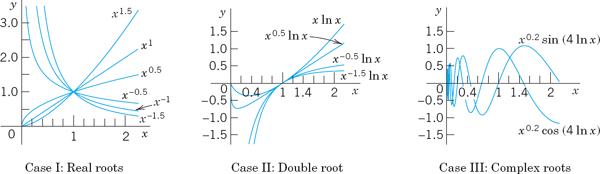
Fig. 48. Euler–Cauchy equations
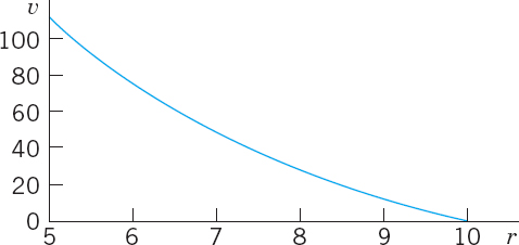
EXAMPLE 4 Boundary Value Problem. Electric Potential Field Between Two Concentric Spheres
Find the electrostatic potential ν = ν(r) between two concentric spheres of radii r1 = 5 cm and r2 = 10 cm kept at potentials ν1 = 110 V and ν2 = 0, respectively.
Physical Information. v (r) is a solution of the Euler–Cauchy equation rν″ + 2ν′ = 0, where ν′ = dv/dr.
Solution. The auxiliary equation is m2 + m = 0. It has the roots 0 and −1. This gives the general solution ν(r) = c1 + c2/r. From the “boundary conditions” (the potentials on the spheres) we obtain
![]()
By subtraction, c2/10 = 110, c2 = 1100. From the second equation, c1 = −c2/10 = −110. Answer: ν(r) = −110 + 1100/rV. Figure 49 shows that the potential is not a straight line, as it would be for a potential between two parallel plates. For example, on the sphere of radius 7.5 cm it is not 110/2 = 55 V, but considerably less. (What is it?)
- Double root. Verify directly by substitution that x(1−a)/2 is a solution of (1) if (2) has a double root, but
 and
and  are not solutions of (1) if the roots m1 and m2 of (2) are different.
2–11 GENERAL SOLUTION
Find a real general solution. Show the details of your work.
- 2. x2y″ − 20y = 0
- 3. 5x2y″ + 23xy′ 16.2y = 0
- 4. xy″ + 2y′ = 0
- 5. 4x2y″ + 5y = 0
- 6. x2y″ + 0.7xy′ − 0.1y = 0
- 7. (x2D2 − 4xD + 6I)y = C
- 8. (x2D2 − 3xD + 4I)y = 0
- 9. (x2D2 − 0.2xD + 0.36I)y = 0
- 10. (x2D2 − xD + 5I)y = 0
- 11. (x2D2 − 3xD + 10I)y = 0
Solve and graph the solution. Show the details of your work.
- 12. x2y″ − 4xy′ + 6y = 0, y(1) = 0.4, y′(1) = 0
- 13. x2y″ + 3xy′ + 0.75y = 0, y(1) = 1, y′(1) = −1.5
- 14. x2y″ + xy′ + 9y = 0, y(1) = 0, y′(1) = 2.5
- 15. x2y″ + 3xy′ + y = 0, y(1) = 3.6, y′(1) = 0.4
- 16. (x2D2 − 3xD + 4I)y = 0, y(1) = −π, y′(1) = 2π
- 17. (x2D2 + xD + I)y = 0, y(1) = 1, y′(1) = 1
- 18. (9x2D2 + 3xD + I)y = 0, y(1) = 1, y′(1) = 0
- 19. (x2D2 − xD − 15I)y = 0, y(1) = 0.1, y′(1) = −4.5
- 20. TEAM PROJECT. Double Root
(a) Derive a second linearly independent solution of (1) by reduction of order; but instead of using (9), Sec. 2.1, perform all steps directly for the present ODE (1).
(b) Obtain xm ln x by considering the solutions xm and xm+s of a suitable Euler–Cauchy equation and letting s → 0.
(c) Verify by substitution that xm ln x, m = (1 − a)/2, is a solution in the critical case.
(d) Transform the Euler–Cauchy equation (1) into an ODE with constant coefficients by setting x = et(x > 0).
(e) Obtain a second linearly independent solution of the Euler–Cauchy equation in the “critical case” from that of a constant-coefficient ODE.
2.6 Existence and Uniqueness of Solutions. Wronskian
In this section we shall discuss the general theory of homogeneous linear ODEs

with continuous, but otherwise arbitrary, variable coefficients p and q. This will concern the existence and form of a general solution of (1) as well as the uniqueness of the solution of initial value problems consisting of such an ODE and two initial conditions

with given x0, K0, and K1.
The two main results will be Theorem 1, stating that such an initial value problem always has a solution which is unique, and Theorem 4, stating that a general solution
![]()
includes all solutions. Hence linear ODEs with continuous coefficients have no “singular solutions” (solutions not obtainable from a general solution).
Clearly, no such theory was needed for constant-coefficient or Euler–Cauchy equations because everything resulted explicitly from our calculations.
Central to our present discussion is the following theorem.
THEOREM 1 Existence and Uniqueness Theorem for Initial Value Problems
If p(x) and q(x) are continuous functions on some open interval I (see Sec. 1.1) and x0 is in I, then the initial value problem consisting of (1) and (2) has a unique solution y(x) on the interval I.
The proof of existence uses the same prerequisites as the existence proof in Sec. 1.7 and will not be presented here; it can be found in Ref. [A11] listed in App. 1. Uniqueness proofs are usually simpler than existence proofs. But for Theorem 1, even the uniqueness proof is long, and we give it as an additional proof in App. 4.
Linear Independence of Solutions
Remember from Sec. 2.1 that a general solution on an open interval I is made up from a basis y1, y2 on I, that is, from a pair of linearly independent solutions on I. Here we call y1, y2 linearly independent on I if the equation
![]()
We call y1, y2 linearly dependent on I if this equation also holds for constants k1, k2 not both 0. In this case, and only in this case, y1 and y2 are proportional on I, that is (see Sec. 2.1),
![]()
For our discussion the following criterion of linear independence and dependence of solutions will be helpful.
THEOREM 2 Linear Dependence and Independence of Solutions
Let the ODE (1) have continuous coefficients p(x) and q(x) on an open interval I. Then two solutions of y1 and y2 of (1) on I are linearly dependent on I if and only if their “Wronskian”

is 0 at some x0 in I. Furthermore, if W = 0 at an x = x0 in I, then W = 0 on I; hence, if there is an x1 in I at which W is not 0, then y1, y2 are linearly independent on I.
PROOF
(a) Let y1 and y2 be linearly dependent on I. Then (5a) or (5b) holds on I. If (5a) holds, then
![]()
Similarly if (5b) holds.
(b) Conversely, we let W(y1, y2) = 0 for some x = x0 and show that this implies linear dependence of y1 and y2 on I. We consider the linear system of equations in the unknowns k1, k2

To eliminate k2, multiply the first equation by y′2 and the second by −y2 and add the resulting equations. This gives
![]()
Similarly, to eliminate k1, multiply the first equation by −y′1 and the second by y1 and add the resulting equations. This gives
![]()
If W were not 0 at x0, we could divide by W and conclude that k1 = k2 = 0. Since W is 0, division is not possible, and the system has a solution for which k1 and k2 are not both 0. Using these numbers k1, k2, we introduce the function
![]()
Since (1) is homogeneous linear, Fundamental Theorem 1 in Sec. 2.1 (the superposition principle) implies that this function is a solution of (1) on I. From (7) we see that it satisfies the initial conditions y(x0) = 0, y′(x0) = 0. Now another solution of (1) satisfying the same initial conditions is y* ≡ 0. Since the coefficients p and q of (1) are continuous, Theorem 1 applies and gives uniqueness, that is, y ≡ y*, written out
![]()
Now since k1 and k2 are not both zero, this means linear dependence of y1, y2 on I.
(c) We prove the last statement of the theorem. If W(x0) = 0 at an x0 in I, we have linear dependence of y1, y2 on I by part (b), hence W ≡ 0 by part (a) of this proof. Hence in the case of linear dependence it cannot happen that W(x1) ≠ 0 at an x1 in I. If it does happen, it thus implies linear independence as claimed.
For calculations, the following formulas are often simpler than (6).

These formulas follow from the quotient rule of differentiation.
Remark. Determinants. Students familiar with second-order determinants may have noticed that

This determinant is called the Wronski determinant5 or, briefly, the Wronskian, of two solutions y1 and y2 of (1), as has already been mentioned in (6). Note that its four entries occupy the same positions as in the linear system (7).
EXAMPLE 1 Illustration of Theorem 2
The functions y1 = cos ωx and y2 = sin ωx are solutions of y″ + ω2y = 0. Their Wronskian is
![]()
Theorem 2 shows that these solutions are linearly independent if and only if ω ≠ 0. Of course, we can see this directly from the quotient y2/y1. For ω = 0 we have y2 = 0, which implies linear dependence (why?).
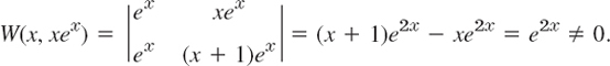
EXAMPLE 2 Illustration of Theorem 2 for a Double Root
A general solution of y″ − 2y′ + y = 0 on any interval is y = (c1 + c2x)ex. (Verify!). The corresponding Wronskian is not 0, which shows linear independence of ex and xex on any interval. Namely,
A General Solution of (1) Includes All Solutions
This will be our second main result, as announced at the beginning. Let us start with existence.
THEOREM 3 Existence of a General Solution
If p(x) and q(x) are continuous on an open interval I, then (1) has a general solution on I.
PROOF
By Theorem 1, the ODE (1) has a solution y1(x) on I satisfying the initial conditions
![]()
and a solution y2(x) on I satisfying the initial conditions
![]()
The Wronskian of these two solutions has at x = x0 the value
![]()
Hence, by Theorem 2, these solutions are linearly independent on I. They form a basis of solutions of (1) on I, and y = c1y1 + c2y2 with arbitrary c1, c2 is a general solution of (1) on I, whose existence we wanted to prove.
We finally show that a general solution is as general as it can possibly be.
THEOREM 4 A General Solution Includes All Solutions
If the ODE (1) has continuous coefficients p(x) and q(x) on some open interval I, then every solution y = Y(x) of (1) on I is of the form
![]()
where y1, y2 is any basis of solutions of (1) on I and C1, C2 are suitable constants.
Hence (1) does not have singular solutions(that is, solutions not obtainable from a general solution).
PROOF
Let y = Y(x) be any solution of (1) on I. Now, by Theorem 3 the ODE (1) has a general solution
![]()
on I. We have to find suitable values of c1, c2 such that y(x) = Y(x) on I. We choose any in I and show first that we can find values of c1, c2 such that we reach agreement at x0, that is, y(x0) and y′(x0) = Y′(x0). Written out in terms of (9), this becomes
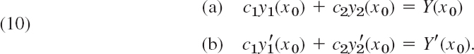
We determine the unknowns c1 and c2. To eliminate c2, we multiply (10a) by y′2(x0) and (10b) by −y2(x0) and add the resulting equations. This gives an equation for c1. Then we multiply (10a) by −y′1(x0) and (10b) by y1(x0) and add the resulting equations. This gives an equation for c2. These new equations are as follows, where we take the values of y1, y′1, y2, y′2, Y, Y′ at x0.

Since y1, y2 is a basis, the Wronskian W in these equations is not 0, and we can solve for c1 and c2. We call the (unique) solution c1 = C1, c2 = C2. By substituting it into (9) we obtain from (9) the particular solution
![]()
Now since C1, C2 is a solution of (10), we see from (10) that
![]()
From the uniqueness stated in Theorem 1 this implies that y* and Y must be equal everywhere on I, and the proof is complete.
Reflecting on this section, we note that homogeneous linear ODEs with continuous variable coefficients have a conceptually and structurally rather transparent existence and uniqueness theory of solutions. Important in itself, this theory will also provide the foundation for our study of nonhomogeneous linear ODEs, whose theory and engineering applications form the content of the remaining four sections of this chapter.
- Derive (6*) from (6).
2–8 BASIS OF SOLUTIONS. WRONSKIAN
Find the Wronskian. Show linear independence by using quotients and confirm it by Theorem 2.
- 2. e4.0x, e−1.5x
- 3. e−0.4x, e−2.6x
- 4. x, 1/x
- 5. x3, x2
- 6. e−x cos ωx, e−x sin ωx
- 7. cosh ax, sinh ax
- 8. xk cos (ln x), xk sin *ln x)
9–15 ODE FOR GIVEN BASIS. WRONSKIAN. IVP
(a) Find a second-order homogeneous linear ODE for which the given functions are solutions. (b) Show linear independence by the Wronskian. (c) Solve the initial value problem.
- 9. cos 5x, sin 5x, y(0) = 3, y′(0) = −5
- 10.

- 11. e−2.5x cos 0.3x, e−2.5x sin 0.3x, y(0) = 3, y′(0) = −7.5
- 12. x2, x2 ln x, y(1) = 4, y′(1) = 6
- 13. 1, e−2x, y(0) = 1, y′(0) = −1
- 14. e−kx cos πx, e−kx sin πx, y(0) = 1, y′(0) = −k − π
- 15. cosh 1.8x, sinh 1.8x, y(0) = 14.20, y′(0) = 16.38
- 16. TEAM PROJECT. Consequences of the Present Theory. This concerns some noteworthy general properties of solutions. Assume that the coefficients p and q of the ODE (1) are continuous on some open interval I, to which the subsequent statements refer.
(a) Solve y″ − y = 0 (a) by exponential functions, (b) by hyperbolic functions. How are the constants in the corresponding general solutions related?
(b) Prove that the solutions of a basis cannot be 0 at the same point.
(c) Prove that the solutions of a basis cannot have a maximum or minimum at the same point.
(d) Why is it likely that formulas of the form (6*) should exist?
(e) Sketch y1(x) = x3 if x
 0 and 0 if x < 0, y2(x) = 0 if x 0 and x3 if x < 0. Show linear independence on −1 < x < 1. What is their Wronskian? What Euler–Cauchy equation do y1, y2 satisfy? Is there a contradiction to Theorem 2?
(f) Prove Abel's formula6

where c = W(y1(x0), y2(x0)). Apply it to Prob. 6. Hint: Write (1) for y1 and for y2. Eliminate q algebraically from these two ODEs, obtaining a first-order linear ODE. Solve it.
2.7 Nonhomogeneous ODEs
We now advance from homogeneous to nonhomogeneous linear ODEs.
Consider the second-order nonhomogeneous linear ODE

where r(x) ![]() 0. We shall see that a “general solution” of (1) is the sum of a general solution of the corresponding homogeneous ODE
0. We shall see that a “general solution” of (1) is the sum of a general solution of the corresponding homogeneous ODE
and a “particular solution” of (1). These two new terms “general solution of (1)” and “particular solution of (1)” are defined as follows.
DEFINITION General Solution, Particular Solution
A general solution of the nonhomogeneous ODE (1) on an open interval I is a solution of the form

here, yh = c1y1 + c2y2 is a general solution of the homogeneous ODE (2) on I and yp is any solution of (1) on I containing no arbitrary constants.
A particular solution of (1) on I is a solution obtained from (3) by assigning specific values to the arbitrary constants c1 and c2 in yh.
Our task is now twofold, first to justify these definitions and then to develop a method for finding a solution yp of (1).
Accordingly, we first show that a general solution as just defined satisfies (1) and that the solutions of (1) and (2) are related in a very simple way.
THEOREM 1 Relations of Solutions of (1) to Those of (2)
- The sum of a solution y of (1) on some open interval I and a solution
 of (2) on I is a solution of (1) on I. In particular, (3) is a solution of (1) on I.
 - The difference of two solutions of (1) on I is a solution of (2) on I.
PROOF
- Let L[y] denote the left side of (1). Then for any solutions y of (1) and of (2) on I,

- For any solutions y and y* of (1) on I we have L[y − y*] = L[y] − L[y*] = r − r = 0.
Now for homogeneous ODEs (2) we know that general solutions include all solutions. We show that the same is true for nonhomogeneous ODEs (1).
THEOREM 2 A General Solution of a Nonhomogeneous ODE Includes All Solutions
If the coefficients p(x), q(x), and the function r(x) in (1) are continuous on some open interval I, then every solution of (1) on I is obtained by assigning suitable values to the arbitrary constants c1 and c2 in a general solution (3) of (1) on I.
PROOF
Let y* be any solution of (1) on I and x0 any x in I. Let (3) be any general solution of (1) on I. This solution exists. Indeed, yh = c1y1 + c2y2 exists by Theorem 3 in Sec. 2.6 because of the continuity assumption, and exists according to a construction to be shown in Sec. 2.10. Now, by Theorem 1(b) just proved, the difference Y = y* − yp is a solution of (2) on I. At x0 we have
![]()
Theorem 1 in Sec. 2.6 implies that for these conditions, as for any other initial conditions in I, there exists a unique particular solution of (2) obtained by assigning suitable values to c1, c2 in yh. From this and y* = Y + yp the statement follows.
Method of Undetermined Coefficients
Our discussion suggests the following. To solve the nonhomogeneous ODE (1) or an initial value problem for (1), we have to solve the homogeneous ODE (2) and find any solution yp of (1), so that we obtain a general solution (3) of (1).
How can we find a solution yp of (1)? One method is the so-called method of undetermined coefficients. It is much simpler than another, more general, method (given in Sec. 2.10). Since it applies to models of vibrational systems and electric circuits to be shown in the next two sections, it is frequently used in engineering.
More precisely, the method of undetermined coefficients is suitable for linear ODEs with constant coefficients a and b

when r(x) is an exponential function, a power of x, a cosine or sine, or sums or products of such functions. These functions have derivatives similar to r(x) itself. This gives the idea. We choose a form for yp similar to r(x), but with unknown coefficients to be determined by substituting that yp and its derivatives into the ODE. Table 2.1 on p. 82 shows the choice of yp for practically important forms of r(x). Corresponding rules are as follows.
Choice Rules for the Method of Undetermined Coefficients
- Basic Rule. If r(x) in (4) is one of the functions in the first column in Table 2.1, choose yp in the same line and determine its undetermined coefficients by substituting yp and its derivatives into (4).
- Modification Rule. If a term in your choice for yp happens to be a solution of the homogeneous ODE corresponding to (4) , multiply this term by x (or by x2 if this solution corresponds to a double root of the characteristic equation of the homogeneous ODE).
- Sum Rule. If r(x) is a sum of functions in the first column of Table 2.1, choose for yp the sum of the functions in the corresponding lines of the second column.
The Basic Rule applies when r(x) is a single term. The Modification Rule helps in the indicated case, and to recognize such a case, we have to solve the homogeneous ODE first. The Sum Rule follows by noting that the sum of two solutions of (1) with r = r1 and r = r2 (and the same left side!) is a solution of (1) with r = r1 + r2. (Verify!)
The method is self-correcting. A false choice for yp or one with too few terms will lead to a contradiction. A choice with too many terms will give a correct result, with superfluous coefficients coming out zero.
Let us illustrate Rules (a)–(c) by the typical Examples 1–3.
Table 2.1 Method of Undetermined Coefficients

EXAMPLE 1 Application of the Basic Rule (a)
Solve the initial value problem
![]()
Solution. Step 1. General solution of the homogeneous ODE. The ODE y″ + y = 0 has the general solution
![]()
Step 2. Solution yp of the nonhomogeneous ODE. We first try yp = Kx2. Then y″p = 2K. By substitution, 2K + Kx2 = 0.001x2. For this to hold for all x, the coefficient of each power of x(x2 and x0) must be the same on both sides; thus K = 0.001 and 2K = 0, a contradiction.
The second line in Table 2.1 suggests the choice
![]()
Equating the coefficients of x2, x, x0 on both sides, we have K2 = 0.001, K1 = 0, 2K2 + K0 = 0. Hence K0 = −2K2 = −0.002. This gives yp = 0.001x2 − 0.002, and
![]()
Step 3. Solution of the initial value problem. Setting x = 0 and using the first initial condition gives y(0) = A − 0.002 = 0, hence A = 0.002. By differentiation and from the second initial condition,
![]()
This gives the answer (Fig. 50)
![]()
Figure 50 shows y as well as the quadratic parabola yp about which y is oscillating, practically like a sine curve since the cosine term is smaller by a factor of about 1/1000.
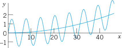
Fig. 50. Solution in Example 1
EXAMPLE 2 Application of the Modification Rule (b)
Solve the initial value problem
![]()
Solution. Step 1. General solution of the homogeneous ODE. The characteristic equation of the homogeneous ODE is λ2 + 3λ + 2.25 = (λ + 1.5)2 = 0. Hence the homogeneous ODE has the general solution
![]()
Step 2. Solution of the nonhomogeneous ODE. The function e−1.5x on the right would normally require the choice Ce−1.5x. But we see from yh that this function is a solution of the homogeneous ODE, which corresponds to a double root of the characteristic equation. Hence, according to the Modification Rule we have to multiply our choice function by x2. That is, we choose
![]()
We substitute these expressions into the given ODE and omit the factor e−1.5x. This yields
![]()
Comparing the coefficients of x2, x, x0 gives 0 = 0, 0 = 0, 2C = −10, hence C = −5. This gives the solution yp = −5x2e−1.5x. Hence the given ODE has the general solution
![]()
Step 3. Solution of the initial value problem. Setting x = 0 in y and using the first initial condition, we obtain y(0) = c1 = 1. Differentiation of y gives
![]()
From this and the second initial condition we have y′(0) = c2 − 1.5c1 = 0. Hence c2 = 1.5c1 = 1.5. This gives the answer (Fig. 51)
![]()
The curve begins with a horizontal tangent, crosses the x-axis at x = 0.6217 (where 1 + 1.5x − 5x2 = 0) and approaches the axis from below as x increases.

Fig. 51. Solution in Example 2
EXAMPLE 3 Application of the Sum Rule (c)
Solve the initial value problem
![]()
Solution. Step 1. General solution of the homogeneous ODE. The characteristic equation of the homogeneous ODE is
![]()
which gives the general solution yh = c1e−x/2 + c2e−3x/2.
Step 2. Particular solution of the nonhomogeneous ODE. We write yp = yp1 + yp2 and, following Table 2.1, (C) and (B),
![]()
Differentiation gives y′p1 = −K sin x + M cos x, y″p1 = −K cos x − M sin x and y′p2 = 1, y″p2 = 0. Substitution of yp1 into the ODE in (7) gives, by comparing the cosine and sine terms,
![]()
hence K = 0 and M = 1. Substituting yp2 into the ODE in (7) and comparing the x- and x0-terms gives
![]()
Hence a general solution of the ODE in (7) is
![]()
Step 3. Solution of the initial value problem. From y, y′ and the initial conditions we obtain
![]()
Hence c1 = 3.1, c2 = 0. This gives the solution of the IVP (Fig. 52)
![]()

Fig. 52. Solution in Example 3
Stability. The following is important. If (and only if) all the roots of the characteristic equation of the homogeneous ODE y″ + ay′ + by = 0 in (4) are negative, or have a negative real part, then a general solution yh of this ODE goes to 0 as x → ∞, so that the “transient solution” y = yh + yp of (4) approaches the “steady-state solution” yp. In this case the nonhomogeneous ODE and the physical or other system modeled by the ODE are called stable; otherwise they are called unstable. For instance, the ODE in Example 1 is unstable.
Applications follow in the next two sections.
1–10 NONHOMOGENEOUS LINEAR ODEs: GENERAL SOLUTION
Find a (real) general solution. State which rule you are using. Show each step of your work.
- y″ + 5y′ + 4y = 10e−3x
- 10y″ + 50y′ + 57.6y = cos x
- y″ + 3y′ + 2y = 12x2
- y″ − 9y = 18 cos πx
- y″ + 4y′ + 4y = e−x cos x


- (3D2 + 27I)y = 3 cos x + cos 3x
- (D2 − 16I)y = 9.6e4x + 30ex
- (D2 + 2D + I)y = 2x sin x
11–18 NONHOMOGENEOUS LINEAR ODEs: IVPs
Solve the initial value problem. State which rule you are using. Show each step of your calculation in detail.
- 11. y″ + 3y = 18x2, y(0) = −3, y′(0) = 0
- 12. y″ + 4y = −12 sin 2x, y(0) = 1.8, y′(0) = 5.0
- 13. 8y″ − 6y′ + y = 6 cosh x, y(0) = 0.2, y′(0) = 0.05
- 14. y″ + 4y′ + 4y = e−2x sin 2x, y(0) = 1, y′(0) = −1.5
- 15. (x2D2 − 3xD + 3I)y = 3 ln x − 4, y(1) = 0, y′(1) = 1; yp = ln x
- 16. (D2 − 2D)y = 6e2x − 4e−2x, y(0) = −1, y′(0) = 6
- 17. (D2 + 0.2D + 0.26I)y = 1.22e0.5x, y(0) = 3.5, y′(0) = 0.35
- 18. (D2 + 2D + 10I)y = 17 sin x − 37 sin 3x, y(0) = 6.6, y′(0) = −2.2
- 19. CAS PROJECT. Structure of Solutions of Initial Value Problems. Using the present method, find, graph, and discuss the solutions y of initial value problems of your own choice. Explore effects on solutions caused by changes of initial conditions. Graph yp, y, y − yp separately, to see the separate effects. Find a problem in which (a) the part of y resulting from yh decreases to zero, (b) increases, (c) is not present in the answer y. Study a problem with y(0) = 0, y′(0) = 0. Consider a problem in which you need the Modification Rule (a) for a simple root, (b) for a double root. Make sure that your problems cover all three Cases I, II, III (see Sec. 2.2).
- 20. TEAM PROJECT. Extensions of the Method of Undetermined Coefficients. (a) Extend the method to products of the function in Table 2.1, (b) Extend the method to Euler–Cauchy equations. Comment on the practical significance of such extensions.
2.8 Modeling: Forced Oscillations. Resonance
In Sec. 2.4 we considered vertical motions of a mass–spring system (vibration of a mass m on an elastic spring, as in Figs. 33 and 53) and modeled it by the homogeneous linear ODE
![]()
Here y(t) as a function of time t is the displacement of the body of mass m from rest.
The mass–spring system of Sec. 2.4 exhibited only free motion. This means no external forces (outside forces) but only internal forces controlled the motion. The internal forces are forces within the system. They are the force of inertia my″, the damping force cy′ (if c > 0), and the spring force ky, a restoring force.

We now extend our model by including an additional force, that is, the external force r(t) on the right. Then we have
![]()
Mechanically this means that at each instant t the resultant of the internal forces is in equilibrium with r(t). The resulting motion is called a forced motion with forcing function r(t) which is also known as input or driving force, and the solution y(t) to be obtained is called the output or the responseof the system to the driving force.
Of special interest are periodic external forces, and we shall consider a driving force of the form
![]()
Then we have the nonhomogeneous ODE

Its solution will reveal facts that are fundamental in engineering mathematics and allow us to model resonance.
Solving the Nonhomogeneous ODE (2)
From Sec. 2.7 we know that a general solution yh of (2) is the sum of a general solution of the homogeneous ODE (1) plus any solution yp of (2). To find yp we use the method of undetermined coefficients (Sec. 2.7), starting from

By differentiating this function (chain rule!) we obtain

Substituting yp, y′p, and y″p into (2) and collecting the cosine and the sine terms, we get
![]()
The cosine terms on both sides must be equal, and the coefficient of the sine term on the left must be zero since there is no sine term on the right. This gives the two equations

for determining the unknown coefficients a and b. This is a linear system. We can solve it by elimination. To eliminate b, multiply the first equation by k − mω2 and the second by −ωc and add the results, obtaining
![]()
Similarly, to eliminate a, multiply (the first equation by ωc and the second by k − mω2 and add to get
![]()
If the factor (k − mω2)2 + ω2c2 is not zero, we can divide by this factor and solve for a and b,
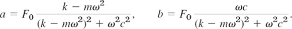
If we set ![]() as in Sec. 2.4, then
as in Sec. 2.4, then ![]() and we obtain
and we obtain
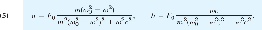
We thus obtain the general solution of the nonhomogeneous ODE (2) in the form
![]()
Here yh is a general solution of the homogeneous ODE (1) and yp is given by (3) with coefficients (5).
We shall now discuss the behavior of the mechanical system, distinguishing between the two cases c = 0 (no damping) and c > 0 (damping). These cases will correspond to two basically different types of output.
Case 1. Undamped Forced Oscillations. Resonance
If the damping of the physical system is so small that its effect can be neglected over the time interval considered, we can set c = 0. Then (5) reduces to ![]() and b = 0. Hence (3) becomes (use
and b = 0. Hence (3) becomes (use ![]() )
)

Here we must assume that ![]() ; physically, the frequency ω/(2π) [cycles/sec] of the driving force is different from the natural frequency ω0/(2π) of the system, which is the frequency of the free undamped motion [see (4) in Sec. 2.4]. From (7) and from (4*) in Sec. 2.4 we have the general solution of the “undamped system”
; physically, the frequency ω/(2π) [cycles/sec] of the driving force is different from the natural frequency ω0/(2π) of the system, which is the frequency of the free undamped motion [see (4) in Sec. 2.4]. From (7) and from (4*) in Sec. 2.4 we have the general solution of the “undamped system”
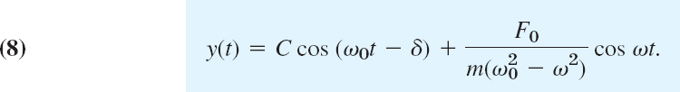
We see that this output is a superposition of two harmonic oscillations of the frequencies just mentioned.
Resonance. We discuss (7). We see that the maximum amplitude of yp is (put cos ωt = 1)

ap depends on ω and ω0. If ω → ω0, then ρ and a0 tend to infinity. This excitation of large oscillations by matching input and natural frequencies (ω = ω0) is called resonance. ρ is called the resonance factor (Fig. 54), and from (9) we see that ρ/k = a0/F0 is the ratio of the amplitudes of the particular solution yp and of the input F0 cos ωt. We shall see later in this section that resonance is of basic importance in the study of vibrating systems.
In the case of resonance the nonhomogeneous ODE (2) becomes

Then (7) is no longer valid, and, from the Modification Rule in Sec. 2.7, we conclude that a particular solution of (10) is of the form
![]()

Fig. 54. Resonance factor ρ(ω)
By substituting this into (10) we find a = 0 and b = F0/(2mω0). Hence (Fig. 55)
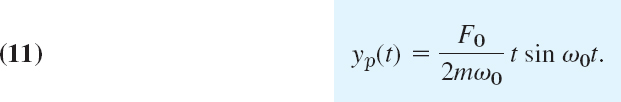

Fig. 55. Particular solution in the case of resonance
We see that, because of the factor t, the amplitude of the vibration becomes larger and larger. Practically speaking, systems with very little damping may undergo large vibrations that can destroy the system. We shall return to this practical aspect of resonance later in this section.
Beats. Another interesting and highly important type of oscillation is obtained if ω is close to ω0. Take, for example, the particular solution [see (8)]

Using (12) in App. 3.1, we may write this as
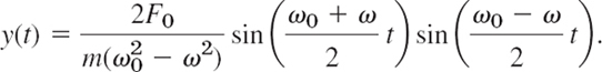
Since ω is close to ω0, the difference ω0 − ω is small. Hence the period of the last sine function is large, and we obtain an oscillation of the type shown in Fig. 56, the dashed curve resulting from the first sine factor. This is what musicians are listening to when they tune their instruments.

Fig. 56. Forced undamped oscillation when the difference of the input and natural frequencies is small (“beats”)
Case 2. Damped Forced Oscillations
If the damping of the mass–spring system is not negligibly small, we have c > 0 and a damping term cy′ in (1) and (2). Then the general solution yh of the homogeneous ODE (1) approaches zero as t goes to infinity, as we know from Sec. 2.4. Practically, it is zero after a sufficiently long time. Hence the “transient solution” (6) of (2), given by y = yh + yp approaches the “steady-state solution” yp. This proves the following.
THEOREM 1 Steady-State Solution
After a sufficiently long time the output of a damped vibrating system under a purely sinusoidal driving force[see (2)]will practically be a harmonic oscillation whose frequency is that of the input.
Amplitude of the Steady-State Solution. Practical Resonance
Whereas in the undamped case the amplitude of yp approaches infinity as ω approaches ω0, this will not happen in the damped case. In this case the amplitude will always be finite. But it may have a maximum for some depending on the damping constant c. This may be called practical resonance. It is of great importance because if c is not too large, then some input may excite oscillations large enough to damage or even destroy the system. Such cases happened, in particular in earlier times when less was known about resonance. Machines, cars, ships, airplanes, bridges, and high-rising buildings are vibrating mechanical systems, and it is sometimes rather difficult to find constructions that are completely free of undesired resonance effects, caused, for instance, by an engine or by strong winds.
To study the amplitude of yp as a function of ω, we write (3) in the form
![]()
C* is called the amplitude of yp and η the phase angle or phase lag because it measures the lag of the output behind the input. According to (5), these quantities are

Let us see whether C*(ω) has a maximum and, if so, find its location and then its size. We denote the radicand in the second root in C* by R. Equating the derivative of C* to zero, we obtain

The expression in the brackets […] is zero if
![]()
By reshuffling terms we have
![]()
The right side of this equation becomes negative if c2 > 2mk, so that then (15) has no real solution and C* decreases monotone as ω increases, as the lowest curve in Fig. 57 shows. If c is smaller, c2 < 2mk, then (15) has a real solution ω = ωmax where

From (15*) we see that this solution increases as c decreases and approaches ω0 as c approaches zero. See also Fig. 57.
The size of C*(ωmax) is obtained from (14), with ![]() given by (15*). For this ω2 we obtain in the second radicand in (14) from (15*)
given by (15*). For this ω2 we obtain in the second radicand in (14) from (15*)
![]()
The sum of the right sides of these two formulas is
![]()
Substitution into (14) gives
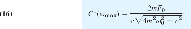
We see that C*(ωmax) is always finite when c > 0. Furthermore, since the expression
![]()
in the denominator of (16) decreases monotone to zero as c2(<2mk) goes to zero, the maximum amplitude (16) increases monotone to infinity, in agreement with our result in Case 1. Figure 57 shows the amplification C*/F0 (ratio of the amplitudes of output and input) as a function of ω for m = 1, k = 1, hence ω0 = 1, and various values of the damping constant c.
Figure 58 shows the phase angle (the lag of the output behind the input), which is less than π/2 when ω < ω0 and greater than π/2 for ω > ω0.
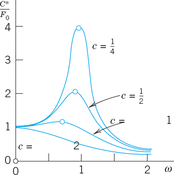
Fig. 57. Amplification C*/F0 as a function of ω for m = 1, k = 1, and various values of the damping constant c

Fig. 58. Phase lag as a function of ω for m = 1, k = 1, thus ω0 = 1, and various values of the damping constant c
- WRITING REPORT. Free and Forced Vibrations. Write a condensed report of 2–3 pages on the most important similarities and differences of free and forced vibrations, with examples of your own. No proofs.
- Which of Probs. 1–18 in Sec. 2.7 (with x = time t) can be models of mass–spring systems with a harmonic oscillation as steady-state solution?
3–7 STEADY-STATE SOLUTIONS
Find the steady-state motion of the mass–spring system modeled by the ODE. Show the details of your work.
- 3. y″ + 6y′ + 8y = 42.5 cos 2t
- 4. y″ + 2.5y′ + 10y = −13.6 sin 4t
- 5. (D2 + D + 4.25I)y = 22.1 cos 4.5t
- 6.

- 7. (4D2 + 12D + 9I)y = 225 − 75 sin 3t
8–15 TRANSIENT SOLUTIONS
Find the transient motion of the mass–spring system modeled by the ODE. Show the details of your work.
- 8. 2y″ + 4y′ + 6.5y = 4 sin 1.5t
- 9. y″ + 3y′ + 3.25y = 3 cos t − 1.5 sin t
- 10. y″ + 16y = 56 cos 4t
- 11.

- 12. (D2 + 2D + 5I)y = 4 cos t + 8 sin t
- 13. (D2 + I)y = cos ωt, ω2 ≠ 1
- 14. (D2 + I)y = 5e−t cos t
- 15. (D2 + 4D + 8I)y = 2 cos 2t + sin 2t
16–20 INITIAL VALUE PROBLEMS
Find the motion of the mass–spring system modeled by the ODE and the initial conditions. Sketch or graph the solution curve. In addition, sketch or graph the curve of y − yp to see when the system practically reaches the steady state.
- 16. y″ + 25y = 25 sin t, y(0) = 1, y′(0) = 1
- 17.
- 18. (D2 + 8D + 17I)y = 474.5 sin 0.5t, y(0) = −5.4, y′(0) = 9.4
- 19.
- 20. (D2 + 5I)y = cos πt − sin πt, y(0) = 0, y′(0) = 0
- 21. Beats. Derive the formula after (12) from (12). Can we have beats in a damped system?
- 22. Beats. Solve y″ + 25y = 99 cos 4.9t, y(0) = 2, y′(0) = 0. How does the graph of the solution change if you change (a) y(0), (b) the frequency of the driving force?
- 23. TEAM EXPERIMENT. Practical Resonance.
(a) Derive, in detail, the crucial formula (16).
(b) By considering dC*/dc show that C*(ωmax) increases as
 decreases.
(c) Illustrate practical resonance with an ODE of your own in which you vary c, and sketch or graph corresponding curves as in Fig. 57.
(d) Take your ODE with c fixed and an input of two terms, one with frequency close to the practical resonance frequency and the other not. Discuss and sketch or graph the output.
(e) Give other applications (not in the book) in which resonance is important.
- 24. Gun barrel. Solve y″ + y = 1 − t2/π2 if 0
 t π and 0 if t → ∞; here, y(0) = 0, y′(0) = 0. This models an undamped system on which a force F acts during some interval of time (see Fig. 59), for instance, the force on a gun barrel when a shell is fired, the barrel being braked by heavy springs (and then damped by a dashpot, which we disregard for simplicity). Hint: At π both y and y′ must be continuous.

- 25. CAS EXPERIMENT. Undamped Vibrations.
(a) Solve the initial value problem y″ + y = cos ωt, ω2 ≠ 1, y(0) = 0, y′(0) = 0. Show that the solution can be written

(b) Experiment with the solution by changing ω to see the change of the curves from those for small ω (>0) to beats, to resonance, and to large values of (see Fig. 60).
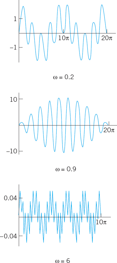
2.9 Modeling: Electric Circuits
Designing good models is a task the computer cannot do. Hence setting up models has become an important task in modern applied mathematics. The best way to gain experience in successful modeling is to carefully examine the modeling process in various fields and applications. Accordingly, modeling electric circuits will be profitable for all students, not just for electrical engineers and computer scientists.
Figure 61 shows an RLC-circuit, as it occurs as a basic building block of large electric networks in computers and elsewhere. An RLC-circuit is obtained from an RL-circuit by adding a capacitor. Recall Example 2 on the RL-circuit in Sec. 1.5: The model of the RL-circuit is LI′ + RI = E(t). It was obtained by KVL (Kirchhoff's Voltage Law)7 by equating the voltage drops across the resistor and the inductor to the EMF (electromotive force). Hence we obtain the model of the RLC-circuit simply by adding the voltage drop Q/C across the capacitor. Here, C F (farads) is the capacitance of the capacitor. Q coulombs is the charge on the capacitor, related to the current by

See also Fig. 62. Assuming a sinusoidal EMF as in Fig. 61, we thus have the model of the RLC-circuit


Fig. 62. Elements in an RLC-circuit

This is an “integro-differential equation.” To get rid of the integral, we differentiate (1′) with respect to t, obtaining

This shows that the current in an RLC-circuit is obtained as the solution of this nonhomogeneous second-order ODE (1) with constant coefficients.
In connection with initial value problems, we shall occasionally use obtained from and

obtained from (1′) and I = Q′.
Solving the ODE (1) for the Current in an RLC-Circuit
A general solution of (1) is the sum I = Ih + Ip where Ih is a general solution of the homogeneous ODE corresponding to (1) and Ip is a particular solution of (1). We first determine Ip by the method of undetermined coefficients, proceeding as in the previous section. We substitute

into (1). Then we collect the cosine terms and equate them to E0ω cos ωt on the right, and we equate the sine terms to zero because there is no sine term on the right,
Before solving this system for a and b, we first introduce a combination of L and C, called the reactance

Dividing the previous two equations by ω ordering them, and substituting S gives
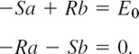
We now eliminate b by multiplying the first equation by S and the second by R, and adding. Then we eliminate a by multiplying the first equation by R and the second by −S and adding. This gives
![]()
We can solve for a and b,

Equation (2) with coefficients a and b given by (4) is the desired particular solution Ip of the nonhomogeneous ODE (1) governing the current I in an RLC-circuit with sinusoidal electromotive force.
Using (4), we can write Ip in terms of “physically visible” quantities, namely, amplitude I0 and phase lag θ of the current behind the EMF, that is,
![]()
where [see (14) in App. A3.1]
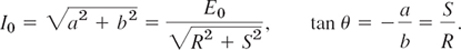
The quantity ![]() is called the impedance. Our formula shows that the impedance equals the ratio E0/I0. This is somewhat analogous to E/I = R (Ohm's law) and, because of this analogy, the impedance is also known as the apparent resistance.
is called the impedance. Our formula shows that the impedance equals the ratio E0/I0. This is somewhat analogous to E/I = R (Ohm's law) and, because of this analogy, the impedance is also known as the apparent resistance.
A general solution of the homogeneous equation corresponding to (1) is
![]()
where λ1 and λ2 are the roots of the characteristic equation
![]()
We can write these roots in the form λ1 = α + β and λ2 = −α − β, where

Now in an actual circuit, R is never zero (hence R > 0). From this it follows that Ih approaches zero, theoretically as t → ∞, but practically after a relatively short time. Hence the transient current I = Ih + Ip tends to the steady-state current Ip, and after some time the output will practically be a harmonic oscillation, which is given by (5) and whose frequency is that of the input (of the electromotive force).
Find the current I(t) in an RLC-circuit with R = 11 Ω (ohms), L = 0.1 H (henry), C = 10−2F (farad), which is connected to a source of EMF E(t) = 110 sin (60 · 2πt) = 110 sin 377 t (hence 60 Hz = 60 cycles/sec, the usual in the U.S. and Canada; in Europe it would be 220 V and 50 Hz). Assume that current and capacitor charge are 0 when t = 0.
Solution. Step 1. General solution of the homogeneous ODE. Substituting R, L, C and the derivative E′(t) into (1), we obtain
![]()
Hence the homogeneous ODE is 0.1I″ + 11I′ + 100I = 0. Its characteristic equation is
![]()
The roots are λ1 = −10 and λ2 = −100. The corresponding general solution of the homogeneous ODE is
![]()
Step 2. Particular solution Ip of (1). We calculate the reactance S = 37.7 − 0.3 = 37.4 and the steady-state current
![]()
with coefficients obtained from (4) (and rounded)
![]()
Hence in our present case, a general solution of the nonhomogeneous ODE (1) is
![]()
Step 3. Particular solution satisfying the initial conditions. How to use Q(0) = 0? We finally determine c1 and c2 from the in initial conditions I(0) = 0 and Q(0) = 0. From the first condition and (6) we have
![]()
We turn to Q(0) = 0. The integral in (1′) equals ∫I dt = Q(t); see near the beginning of this section. Hence for t = 0, Eq. (1′) becomes
![]()
Differentiating (6) and setting t = 0, we thus obtain
![]()
The solution of this and (7) is c1 = −0.323, c2 = 3.033. Hence the answer is
![]()
You may get slightly different values depending on the rounding. Figure 63 shows I(t) as well as Ip(t), which practically coincide, except for a very short time near t = 0 because the exponential terms go to zero very rapidly. Thus after a very short time the current will practically execute harmonic oscillations of the input frequency 60 Hz = 60 cycles/sec. Its maximum amplitude and phase lag can be seen from (5), which here takes the form
![]()

Fig. 63. Transient (upper curve) and steady-state currents in Example 1
Analogy of Electrical and Mechanical Quantities
Entirely different physical or other systems may have the same mathematical model. For instance, we have seen this from the various applications of the ODE y′ = ky in Chap. 1. Another impressive demonstration of this unifying power of mathematics is given by the ODE (1) for an electric RLC-circuit and the ODE (2) in the last section for a mass–spring system. Both equations
![]()
are of the same form. Table 2.2 shows the analogy between the various quantities involved. The inductance L corresponds to the mass m and, indeed, an inductor opposes a change in current, having an “inertia effect” similar to that of a mass. The resistance R corresponds to the damping constant c, and a resistor causes loss of energy, just as a damping dashpot does. And so on.
This analogy is strictly quantitative in the sense that to a given mechanical system we can construct an electric circuit whose current will give the exact values of the displacement in the mechanical system when suitable scale factors are introduced.
The practical importance of this analogy is almost obvious. The analogy may be used for constructing an “electrical model” of a given mechanical model, resulting in substantial savings of time and money because electric circuits are easy to assemble, and electric quantities can be measured much more quickly and accurately than mechanical ones.
Table 2.2 Analogy of Electrical and Mechanical Quantities
| Electrical System | Mechanical System |
| Inductance L | Mass m |
| Resistance R | Damping constant c |
| Reciprocal 1/C of capacitance | Spring modulus k |
| Driving force F0 cos ωt | |
| Current I(t) | Displacement y(t) |
Related to this analogy are transducers, devices that convert changes in a mechanical quantity (for instance, in a displacement) into changes in an electrical quantity that can be monitored; see Ref. [GenRef11] in App. 1.
1–6 RLC-CIRCUITS: SPECIAL CASES
- RC-Circuit. Model the RC-circuit in Fig. 64. Find the current due to a constant E.


- RC-Circuit. Solve Prob. 1 when E = E0 sin ωt and R, C, E0, and ω are arbitrary.
- RL-Circuit. Model the RL-circuit in Fig. 66. Find a general solution when R, L, E are any constants. Graph or sketch solutions when L = 0.25 H, R = 10 Ω, and E = 48 V.


- RL-Circuit. Solve Prob. 3 when E = E0 sin ωt and R, L, E0, and are arbitary. Sketch a typical solution.

- LC-Circuit. This is an RLC-circuit with negligibly small R (analog of an undamped mass–spring system). Find the current when L = 0.5 H, C = 0.005 F, and E = sin t V, assuming zero initial current and charge.

- LC-Circuit. Find the current when L = 0.5 H, C = 0.005 F, E = 2t2 V, and initial current and charge zero.
7–18 GENERAL RLC-CIRCUITS
- 7. Tuning. In tuning a stereo system to a radio station, we adjust the tuning control (turn a knob) that changes C (or perhaps L) in an RLC-circuit so that the amplitude of the steady-state current (5) becomes maximum. For what C will this happen?
8–14 Find the steady-state current in the RLC-circuit in Fig. 61 for the given data. Show the details of your work.
- 8. R = 4 Ω, L = 0.5 H, C = 0.1 F, E = 500 sin 2t V
- 9. R = 4 Ω L = 0.1 H, C = 0.05 F, E = 110 V
- 10. R = 2 Ω, L = 1 H,
 E = 157 sin 3t V
 - 11.

- 12. R = 0.2 Ω, L = 0.1 H, C = 2 F, E = 220 sin 314t V
- 13.
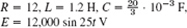
- 14. Prove the claim in the text that if R ≠ 0 (hence R > 0), then the transient current approaches Ip as t → ∞.
- 15. Cases of damping. What are the conditions for an RLC-circuit to be (I) overdamped, (II) critically damped, (III) underdamped? What is the critical resistance Rcrit (the analog of the critical damping constant
 )?
)?
16–18 Solve the initial value problem for the RLC-circuit in Fig. 61 with the given data, assuming zero initial current and charge. Graph or sketch the solution. Show the details of your work.
- 16. R = 8 Ω, L = 0.2 H, C = 12.5 · 10−3F, E = 100 sin 10t V
- 17. R = 6 Ω, L = 1 H, C = 0.04 F, E = 600 (cos t + 4 sin t) V
- 18. R = 18 Ω, L = 1 H, C = 12.5 · 10−3F, E = 820 cos 10t V
- 19. WRITING REPORT. Mechanic-Electric Analogy. Explain Table 2.2 in a 1–2 page report with examples, e.g., the analog (with L = 1 H) of a mass–spring system of mass 5 kg, damping constant 10 kg sec, spring constant 60 kg/sec2, and driving force 220 cos 10t kg/sec.
- 20. Complex Solution Method. Solve

 , by substituting Ip = Keiωt (K unknown) and its derivatives and taking the real part Ip of the solution
  . Show agreement with (2), (4). Hint: Use (11) eiωt = cos ωt + i sin ωt; cf. Sec. 2.2, and i2 = −1.
2.10 Solution by Variation of Parameters
We continue our discussion of nonhomogeneous linear ODEs, that is

In Sec. 2.6 we have seen that a general solution of (1) is the sum of a general solution of the corresponding homogeneous ODE and any particular solution yp of (1). To obtain yp when r(x) is not too complicated, we can often use the method of undetermined coefficients, as we have shown in Sec. 2.7 and applied to basic engineering models in Secs. 2.8 and 2.9.
However, since this method is restricted to functions r(x) whose derivatives are of a form similar to r(x) itself (powers, exponential functions, etc.), it is desirable to have a method valid for more general ODEs (1), which we shall now develop. It is called the method of variation of parameters and is credited to Lagrange (Sec. 2.1). Here p, q, r in (1) may be variable (given functions of x), but we assume that they are continuous on some open interval I.
Lagrange's method gives a particular solution yp of (1) on I in the form

where y1, y2 form a basis of solutions of the corresponding homogeneous ODE
![]()
on I, and W is the Wronskian of y1, y2,
![]()
CAUTION! The solution formula (2) is obtained under the assumption that the ODE is written in standard form, with y″ as the first term as shown in (1). If it starts with f(x)y″, divide first by f(x).
The integration in (2) may often cause difficulties, and so may the determination of y1, y2 if (1) has variable coefficients. If you have a choice, use the previous method. It is simpler. Before deriving (2) let us work an example for which you do need the new method. (Try otherwise.)
EXAMPLE 1 Method of Variation of Parameters
Solve the nonhomogeneous ODE
![]()
Solution. A basis of solutions of the homogeneous ODE on any interval is y1 = cos x, y2 = sin x. This gives the Wronskian
![]()
From (2), choosing zero constants of integration, we get the particular solution of the given ODE
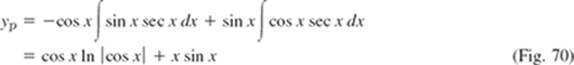
Figure 70 shows yp and its first term, which is small, so that x sin x essentially determines the shape of the curve of yp. (Recall from Sec. 2.8 that we have seen x sin x in connection with resonance, except for notation.) From yp and the general solution yh = c1y1 + c2y2 of the homogeneous ODE we obtain the answer
![]()
Had we included integration constants −c1, c2 in (2), then (2) would have given the additional c1 cos x + c2 sin x = c1y1 + c2y2 that is, a general solution of the given ODE directly from (2). This will always be the case.
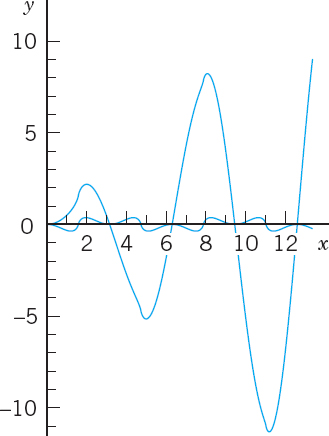
Fig. 70. Particular solution yp and its first term in Example 1
Idea of the Method. Derivation of (2)
What idea did Lagrange have? What gave the method the name? Where do we use the continuity assumptions?
The idea is to start from a general solution
![]()
of the homogeneous ODE (3) on an open interval I and to replace the constants (“the parameters”) c1 and c2 by functions u(x) and ν(x); this suggests the name of the method. We shall determine u and v so that the resulting function
![]()
is a particular solution of the nonhomogeneous ODE (1). Note that yh exists by Theorem 3 in Sec. 2.6 because of the continuity of p and q on I. (The continuity of r will be used later.)
We determine u and v by substituting (5) and its derivatives into (1). Differentiating (5), we obtain
![]()
Now yp must satisfy (1). This is one condition for two functions u and v. It seems plausible that we may impose a second condition. Indeed, our calculation will show that we can determine u and v such that yp satisfies (1) and u and v satisfy as a second condition the equation
![]()
This reduces the first derivative y′p to the simpler form
![]()
Differentiating (7), we obtain
![]()
We now substitute yp and its derivatives according to (5), (7), (8) into (1). Collecting terms in u and terms in v, we obtain
![]()
Since y1 and y2 are solutions of the homogeneous ODE (3), this reduces to
![]()
Equation (6) is
![]()
This is a linear system of two algebraic equations for the unknown functions u′ and v′ We can solve it by elimination as follows (or by Cramer's rule in Sec. 7.6). To eliminate v′ we multiply (9a) by −y2 and (9b) by y′2 and add, obtaining
![]()
Here, W is the Wronskian (4) of y1, y2. To eliminate u′ we multiply (9a) by y1 and (9b) by −y′1 and add, obtaining
Since y1, y2 form a basis, we have W ≠ 0 (by Theorem 2 in Sec. 2.6) and can divide by W,

By integration,

These integrals exist because r(x) is continuous. Inserting them into (5) gives (2) and completes the derivation.
1–13 GENERAL SOLUTION
Solve the given nonhomogeneous linear ODE by variation of parameters or undetermined coefficients. Show the details of your work.
- y″ + 9y = sec 3x
- y″ + 9y = csc 3x
- x2y″ − 2xy′ + 2y = x3 sin x
- y″ − 4y′ + 5y = e2x csc x
- y″ + y = cos x − sin x
- (D2 + 6D + 9I)y = 16e−3x/(x2 + 1)
- (D2 − 4D + 4I)y = 6e2x/x4
- (D2 + 4I)y = cosh 2x
- (D2 − 2D + I)y = 35x3/2ex
- (D2 + 2D + 2I)y = 4e−x sec3x
- (x2D2 − 4xD + 6I)y = 21x−4
- (D2 − I)y = 1/cosh x
- (x2D2 + xD − 9I)y = 38x5
- TEAM PROJECT. Comparison of Methods. Invention. The undetermined-coefficient method should be used whenever possible because it is simpler. Compare it with the present method as follows.
(a) Solve y″ + 4y′ + 3y = 65 cos 2x by both methods, showing all details, and compare.
(b) Solve y″ − 2y′ + y = r1 + r2, r1 = 35x3/2exr2 = x2 by applying each method to a suitable function on the right.
(c) Experiment to invent an undetermined-coefficient method for nonhomogeneous Euler–Cauchy equations.
CHAPTER 2 REVIEW QUESTIONS AND PROBLEMS
- Why are linear ODEs preferable to nonlinear ones in modeling?
- What does an initial value problem of a second-order ODE look like? Why must you have a general solution to solve it?
- By what methods can you get a general solution of a nonhomogeneous ODE from a general solution of a homogeneous one?
- Describe applications of ODEs in mechanical systems. What are the electrical analogs of the latter?
- What is resonance? How can you remove undesirable resonance of a construction, such as a bridge, a ship, or a machine?
- What do you know about existence and uniqueness of solutions of linear second-order ODEs?
7–18 GENERAL SOLUTION
Find a general solution. Show the details of your calculation.
- 7. 4y″ + 32y′ + 63y = 0
- 8. y″ + y′ − 12y = 0
- 9. y″ + 6y′ + 34y = 0
- 10. y″ + 0.20y′ + 0.17y = 0
- 11. (100D2 − 160D + 64I)y = 0
- 12. (D2 + 4πD + 4π2I)y = 0
- 13. (x2D2 + 2xD − 12I)y = 0
- 14. (x2D2 + xD − 9I)y = 0
- 15. (2D2 − 3D − 2I)y = 13 − 2x2
- 16. (D2 + 2D + 2I)y = 3e−x cos 2x
- 17. (4D2 − 12D + 9I)y = 2e1.5x
- 18. yy″ = 2y′2
Solve the problem, showing the details of your work. Sketch or graph the solution.
- 19. y″ + 16y = 17ex, y(0) = 6, y′(0) = −2
- 20. y″ − 3y′ + 2y = 10 sin x, y(0) = 1, y′(0) = −6
- 21. (x2D2 + xD − I)y = 16x3, y(1) = −1, y′(1) = 1
- 22. (x2D2 + 15xD + 49I)y = 0, y(1) = 2, y′(1) = −11
23–30 APPLICATIONS
- 23. Find the steady-state current in the RLC-circuit in Fig. 71 when R =2 kΩ (2000 Ω), L = 1 H, C = 4 · 10−3F, and E = 110 sin 415t V (66 cycles sec).
- 24. Find a general solution of the homogeneous linear ODE corresponding to the ODE in Prob. 23.
- 25. Find the steady-state current in the RLC-circuit in Fig. 71 when R = 50 Ω, L = 30 H, C = 0.025 F, E = 200 sin 4t V.
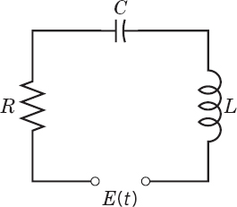
- 26. Find the current in the RLC-circuit in Fig. 71 when R = 40 Ω, L = 0.4 H, C = 10−4 F, E = 220 sin 314t V (50 cycles sec).
- 27. Find an electrical analog of the mass–spring system with mass 4 kg, spring constant 10 kg/sec2, damping constant 20 kg/sec, and driving force 100 sin 4t nt.
- 28. Find the motion of the mass–spring system in Fig. 72 with mass 0.125 kg, damping 0, spring constant 1.125 kg/sec2, and driving force cos t − 4 sin t nt, assuming zero initial displacement and velocity. For what frequency of the driving force would you get resonance?

- 29. Show that the system in Fig. 72 with m = 4, c = 0, k = 36, and driving force 61 cos 3.1t exhibits beats. Hint: Choose zero initial conditions.
- 30. In Fig. 72, let m = 1 kg, c = 4 kg/sec, k = 24 kg/sec2, and r(t) = 10 cos ωt nt. Determine w such that you get the steady-state vibration of maximum possible amplitude. Determine this amplitude. Then find the general solution with this ω and check whether the results are in agreement.
SUMMARY OF CHAPTER 2 Second-Order Linear ODEs
Second-order linear ODEs are particularly important in applications, for instance, in mechanics (Secs. 2.4, 2.8) and electrical engineering (Sec. 2.9). A second-order ODE is called linear if it can be written
![]()
(If the first term is, say, f(x)y″ divide by f(x) to get the “standard form” (1) with y″ as the first term.) Equation (1) is called homogeneous if r(x) is zero for all x considered, usually in some open interval; this is written r(x) ≡ 0. Then
![]()
Equation (1) is called nonhomogeneous if r(x) ![]() 0 (meaning r(x) is not zero for some x considered).
0 (meaning r(x) is not zero for some x considered).
For the homogeneous ODE (2) we have the important superposition principle (Sec. 2.1) that a linear combination y = ky1 + ly2 of two solutions y1, y2 is again a solution.
Two linearly independent solutions y1, y2 of (2) on an open interval I form a basis (or fundamental system) of solutions on I. and y = c1y1 + c2y2 with arbitrary constants c1, c2 a general solution of (2) on I. From it we obtain a particular solution if we specify numeric values (numbers) for c1 and c2 usually by prescribing two initial conditions
![]()
(2) and (3) together form an initial value problem. Similarly for (1) and (3).
For a nonhomogeneous ODE (1) a general solution is of the form
![]()
Here yh is a general solution of (2) and yp is a particular solution of (1). Such a yp can be determined by a general method (variation of parameters, Sec. 2.10) or in many practical cases by the method of undetermined coefficients. The latter applies when (1) has constant coefficients p and q, and r(x) is a power of x, sine, cosine, etc. (Sec. 2.7). Then we write (1) as
![]()
The corresponding homogeneous ODE y′ + ay′ + by = 0 has solutions y = eλx, where λ is a root of
![]()
Hence there are three cases (Sec. 2.2):
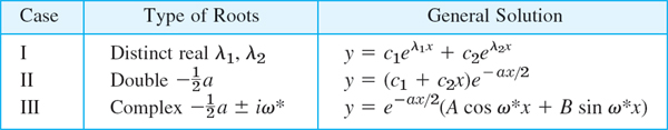
Here ω* is used since ω is needed in driving forces.
Important applications of (5) in mechanical and electrical engineering in connection with vibrations and resonance are discussed in Secs. 2.4, 2.7, and 2.8.
Another large class of ODEs solvable “algebraically” consists of the Euler–Cauchy equations
![]()
These have solutions of the form y = xm where m is a solution of the auxiliary equation
![]()
Existence and uniqueness of solutions of (1) and (2) is discussed in Secs. 2.6 and 2.7, and reduction of order in Sec. 2.1.
1 Credited to the great mathematician JOSEPH LOUIS LAGRANGE (1736–1813), who was born in Turin, of French extraction, got his first professorship when he was 19 (at the Military Academy of Turin), became director of the mathematical section of the Berlin Academy in 1766, and moved to Paris in 1787. His important major work was in the calculus of variations, celestial mechanics, general mechanics (Mécanique analytique, Paris, 1788), differential equations, approximation theory, algebra, and number theory.
2 ROBERT HOOKE (1635–1703), English physicist, a forerunner of Newton with respect to the law of gravitation.
3 HEINRICH HERTZ (1857–1894), German physicist, who discovered electromagnetic waves, as the basis of wireless communication developed by GUGLIELMO MARCONI (1874–1937), Italian physicist (Nobel prize in 1909).
4LEONHARD EULER (1707–1783) was an enormously creative Swiss mathematician. He made fundamental contributions to almost all branches of mathematics and its application to physics. His important books on algebra and calculus contain numerous basic results of his own research. The great French mathematician AUGUSTIN LOUIS CAUCHY (1789–1857) is the father of modern analysis. He is the creator of complex analysis and had great influence on ODEs, PDEs, infinite series, elasticity theory, and optics.
5Introduced by WRONSKI (JOSEF MARIA HÖNE, 1776–1853), Polish mathematician.
6NIELS HENRIK ABEL (1802–1829), Norwegian mathematician.
7GUSTAV ROBERT KIRCHHOFF (1824–1887), German physicist. Later we shall also need Kirchhoff's Current Law (KCL):
At any point of a circuit, the sum of the inflowing currents is equal to the sum of the outflowing currents.
The units of measurement of electrical quantities are named after ANDRÉ MARIE AMPÈRE (1775–1836), French physicist, CHARLES AUGUSTIN DE COULOMB (1736–1806), French physicist and engineer, MICHAEL FARADAY (1791–1867), English physicist, JOSEPH HENRY (1797–1878), American physicist, GEORG SIMON OHM (1789–1854), German physicist, and ALESSANDRO VOLTA (1745–1827), Italian physicist.