
APPENDIX 4
Additional Proofs

PROOF OF THEOREM 1 Uniqueness1
Assuming that the problem consisting of the ODE
![]()
and the two initial conditions
![]()
has two solutions y1(x) and y2(x) on the interval I in the theorem, we show that their difference
![]()
is identically zero on I; then y1 ≡ y2 on I, which implies uniqueness.
Since (1) is homogeneous and linear, y is a solution of that ODE on I, and since y1 and y2 satisfy the same initial conditions, y satisfies the conditions
![]()
We consider the function
![]()
and its derivative
![]()
From the ODE we have
![]()
By substituting this in the expression for z′ we obtain
![]()
Now, since y and y′ are real,
![]()
From this and the definition of z we obtain the two inequalities
![]()
From (13b) we have 2yy′ ![]() −z. Together, |2yy′|
−z. Together, |2yy′| ![]() z. For the last term in (12) we now obtain
z. For the last term in (12) we now obtain
![]()
Using this result as well as −p ![]() |p| and applying (13a) to the term 2yy′ in (12), we find
|p| and applying (13a) to the term 2yy′ in (12), we find
![]()
Since y′2 ![]() y2 + y′2 = z, from this we obtain
y2 + y′2 = z, from this we obtain
![]()
or, denoting the function in parentheses by h,
![]()
Similarly, from (12) and (13) it follows that
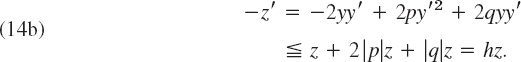
The inequalities (14a) and (14b) are equivalent to the inequalities
![]()
Integrating factors for the two expressions on the left are
![]()
The integrals in the exponents exist because h is continuous. Since F1 and F2 are positive, we thus have from (15)
![]()
This means that F1z is nonincreasing and F2z is nondecreasing on I. Since z(x0) = 0 by (11), when x ![]() x0 we thus obtain
x0 we thus obtain
![]()
and similarly, when x ![]() x0,
x0,
![]()
Dividing by F1 and F2 and noting that these functions are positive, we altogether have
![]()
This implies that z =y2 + y ′2 ≡ 0 on I. Hence y ≡ 0 or y1 ≡ y2 on I.
PROOF OF THEOREM 2 Frobenius Method. Basis of Solutions. Three Cases
The formula numbers in this proof are the same as in the text of Sec. 5.3. An additional formula not appearing in Sec. 5.3 will be called (A) (see below).
The ODE in Theorem 2 is
![]()
where b(x) and c(x) are analytic functions. We can write it
![]()
The indicial equation of (1) is
![]()
The roots r1, r2 of this quadratic equation determine the general form of a basis of solutions of (1), and there are three possible cases as follows.
Case 1. Distinct Roots Not Differing by an Integer. A first solution of (1) is of the form
![]()
and can be determined as in the power series method. For a proof that in this case, the ODE (1) has a second independent solution of the form
![]()
see Ref. [A11] listed in App. 1.
Case 2. Double Root. The indicial equation (4) has a double root r if and only if (b0 − 1)2 − 4c0 = 0, and then ![]() A first solution
A first solution
![]()
can be determined as in Case 1. We show that a second independent solution is of the form
![]()
We use the method of reduction of order (see Sec. 2.1), that is, we determine u(x) such that y2(x) = u(x)y1(x) is a solution of (1). By inserting this and the derivatives
![]()
into the ODE (1′) we obtain
![]()
Since y1 is a solution of (1′), the sum of the terms involving u is zero, and this equation reduces to
![]()
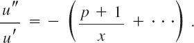
By dividing by x2y1 and inserting the power series for b we obtain
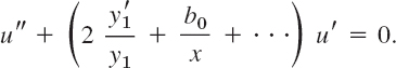
Here, and in the following, the dots designate terms that are constant or involve positive powers of x. Now, from (7), it follows that

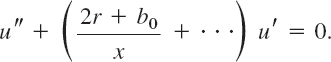
Hence the previous equation can be written
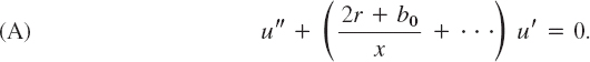
Since r = (1 − b0)/2, the term (2r + b0)/x equals 1/x, and by dividing by u′ we thus have

By integration we obtain ln u′ = −ln x + …, hence u′ = (1/x) e(…). Expanding the exponential function in powers of x and integrating once more, we see that u is of the form
![]()
Inserting this into y2 =uy1, we obtain for y2 a representation of the form (8).
Case 3. Roots Differing by an Integer. We write r1 = r and r2 = r − p where p is a positive integer. A first solution
![]()
can be determined as in Cases 1 and 2. We show that a second independent solution is of the form
![]()
where we may have k ≠ 0 or k = 0. As in Case 2 we set y2 = uy1. The first steps are literally as in Case 2 and give Eq. (A),
Now by elementary algebra, the coefficient b0 − 1 of r in (4) equals minus the sum of the roots,
![]()
Hence 2r + b0 = p + 1, and division by u′ gives
The further steps are as in Case 2. Integrating, we find
![]()
where dots stand for some series of nonnegative integer powers of x. By expanding the exponential function as before we obtain a series of the form
![]()
We integrate once more. Writing the resulting logarithmic term first, we get

Hence, by (9) we get for y2 = uy1 the formula
![]()
But this is of the form (10) with k = kp since r1 − p = r2 and the product of the two series involves nonnegative integer powers of x only.
The definition of a determinant

as given in Sec. 7.7 is unambiguous, that is, it yields the same value of D no matter which rows or columns we choose in the development.
In this proof we shall use formula numbers not yet used in Sec. 7.7.
We shall prove first that the same value is obtained no matter whichrow is chosen.
The proof is by induction. The statement is true for a second-order determinant, for which the developments by the first row a11a22 + a12(−a21) and by the second row a21(−a12) + a22a11 give the same value a11a22 −a12a21. Assuming the statement to be true for an (n − 1) st-order determinant, we prove that it is true for an nth-order determinant.
For this purpose we expand D in terms of each of two arbitrary rows, say, the ith and the jth, and compare the results. Without loss of generality let us assume i < j.
First Expansion. We expand D by the ith row. A typical term in this expansion is
![]()
The minor Mik of aik in D is an (n − 1)st-order determinant. By the induction hypothesis we may expand it by any row. We expand it by the row corresponding to the jth row of D. This row contains the entries ajl (l ≠ k). It is the (j − 1) st row of Mik, because Mik does not contain entries of the ith row of D, and i < j. We have to distinguish between two cases as follows.
Case I. If l < k, then the entry aij belongs to the lth column of Mik (see Fig. 561). Hence the term involving ajl in this expansion is
![]()
where Mikjl is the minor of ajl in Mik. Since this minor is obtained from Mik by deleting the row and column of ajl, it is obtained from D by deleting the ith and jth rows and the kth and lth columns of D. We insert the expansions of the Mik into that of D. Then it follows from (19) and (20) that the terms of the resulting representation of D are of the form
![]()
where
![]()
Case II. If l > k, the only difference is that then ajl belongs to the (l − 1)st column of Mik, because Mik does not contain entries of the kth column of D, and k < l. This causes an additional minus sign in (20), and, instead of (21a), we therefore obtain
![]()
where b is the same as before.

Fig. 561. Cases I and II of the two expansions of D
Second Expansion. We now expand D at first by the jth row. A typical term in this expansion is
![]()
By the induction hypothesis we may expand the minor Mjl of ajl in D by its ith row, which corresponds to the ith row of D, since j > i.
Case I. If k > l, the entry ajk in that row belongs to the (k − 1)st column of Mjl, because Mjl does not contain entries of the lth column of D, and l < k (see Fig. 561). Hence the term involving ap in this expansion is
![]()
where the minor Mikjl of ajk in Mjl is obtained by deleting the ith and jth rows and the kth and lth columns of D [and is, therefore, identical with Mikjl in (20), so that our notation is consistent]. We insert the expansions of the Mjl into that of D. It follows from (22) and (23) that this yields a representation whose terms are identical with those given by (21a) when l <k.
Case II. If k < l, then aik belongs to the kth column of Mjl, we obtain an additional minus sign, and the result agrees with that characterized by (21b).
We have shown that the two expansions of D consist of the same terms, and this proves our statement concerning rows.
The proof of the statement concerning columns is quite similar; if we expand D in terms of two arbitrary columns, say, the kth and the lth, we find that the general term involving ajlaik is exactly the same as before. This proves that not only all column expansions of D yield the same value, but also that their common value is equal to the common value of the row expansions of D.
This completes the proof and shows that our definition of an nth-order determinant is unambiguous.
We prove that in right-handed Cartesian coordinates, the vector product
![]()
has the components
![]()
We need only consider the case v ≠ 0. Since v is perpendicular to both a and b, Theorem 1 in Sec. 9.2 gives a · v = 0 and b · v = 0; in components [see (2), Sec. 9.2],

Multiplying the first equation by b3, the last by a3, and subtracting, we obtain
![]()
Multiplying the first equation by b1, the last by a1, and subtracting, we obtain
![]()
We can easily verify that these two equations are satisfied by
![]()
where c is a constant. The reader may verify, by inserting, that (4) also satisfies (3). Now each of the equations in (3) represents a plane through the origin in v1v2v3-space. The vectors a and b are normal vectors of these planes (see Example 6 in Sec. 9.2). Since v ≠ 0, these vectors are not parallel and the two planes do not coincide. Hence their intersection is a straight line L through the origin. Since (4) is a solution of (3) and, for varying c, represents a straight line, we conclude that (4) represents L, and every solution of (3) must be of the form (4). In particular, the components of v must be of this form, where c is to be determined. From (4) we obtain
![]()
This can be written
![]()
as can be verified by performing the indicated multiplications in both formulas and comparing. Using (2) in Sec. 9.2, we thus have
![]()
By comparing this with formula (12) in Prob. 4 of Problem Set 9.3 we conclude that c = ±1.
We show that c = +1. This can be done as follows.
If we change the lengths and directions of a and b continuously and so that at the end a = i and b = j (Fig. 188a in Sec. 9.3), then v will change its length and direction continuously, and at the end, v = i × j = k. Obviously we may effect the change so that both a and b remain different from the zero vector and are not parallel at any instant. Then v is never equal to the zero vector, and since the change is continuous and c can only assume the values +1 or −1, it follows that at the end c must have the same value as before. Now at the end a = i, b = j, v = k and, therefore, a1 = 1, b2 = 1, v3 = 1, and the other components in (4) are zero. Hence from (4) we see that v3 =c = +1. This proves Theorem 1.
For a left-handed coordinate system, i × j = − k (see Fig. 188b in Sec. 9.3), resulting in c = −1. This proves the statement right after formula (2).
PROOF OF THE INVARIANCE OF THE CURL
This proof will follow from two theorems (A and B), which we prove first.
THEOREM A Transformation Law for Vector Components
For any vector v the components v1, v2, v3 and ![]() in any two systems of Cartesian coordinates x1, x2, x3 and
in any two systems of Cartesian coordinates x1, x2, x3 and ![]() , respectively, are related by
, respectively, are related by

and conversely

with coefficients

satisfying

where the Kronecker delta2is given by
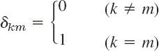
and i, j, k and i*, j*, k* denote the unit vectors in the positive ![]() and
and ![]() -directions, respectively.
-directions, respectively.
The representation of v in the two systems are
![]()
Since i* · i* = 1, i* · j* = 0, i* · k* = 0, we get from (5b) simply i* · v = v1* and from this and (5a)
![]()
Because of (3), this is the first formula in (1), and the other two formulas are obtained similarly, by considering j* · v and then k* · v. Formula (2) follows by the same idea, taking i · v = v1 from (5a) and then from (5b) and (3)
![]()
and similarly for the other two components.
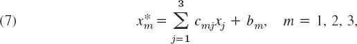
We prove (4). We can write (1) and (2) briefly as

Substituting vj into ![]() , we get
, we get

where k = 1, 2, 3. Taking k = 1, we have

For this to hold for every vector v, the first sum must be 1 and the other two sums 0. This proves (4) with k = 1 for m = 1, 2, 3. Taking k = 2 and then k = 3, we obtain (4) with k = 2 and 3, for m = 1, 2, 3.
THEOREM B Transformation Law for Cartesian Coordinates
The transformation of any Cartesian x1x2x3-coordinate system into any other Cartesian ![]() -coordinate system is of the form
-coordinate system is of the form
with coefficients (3) and constants b1, b2, b3; conversely,

Theorem B follows from Theorem A by noting that the most general transformation of a Cartesian coordinate system into another such system may be decomposed into a transformation of the type just considered and a translation; and under a translation, corresponding coordinates differ merely by a constant.
PROOF OF THE INVARIANCE OF THE CURL
We write again x1, x2, x3 instead of x, y, z, and similarly ![]() for other Cartesian coordinates, assuming that both systems are right-handed. Let a1, a2, a3 denote the components of curl v in the x1x2x3-coordinates, as given by (1), Sec. 9.9, with
for other Cartesian coordinates, assuming that both systems are right-handed. Let a1, a2, a3 denote the components of curl v in the x1x2x3-coordinates, as given by (1), Sec. 9.9, with
![]()
Similarly, let ![]() denote the components of curl v in the
denote the components of curl v in the ![]() -coordinate system. We prove that the length and direction of curlv are independent of the particular choice of Cartesian coordinates, as asserted. We do this by showing that the components of curl v satisfy the transformation law (2), which is characteristic of vector components. We consider a1. We use (6a), and then the chain rule for functions of several variables (Sec. 9.6). This gives
-coordinate system. We prove that the length and direction of curlv are independent of the particular choice of Cartesian coordinates, as asserted. We do this by showing that the components of curl v satisfy the transformation law (2), which is characteristic of vector components. We consider a1. We use (6a), and then the chain rule for functions of several variables (Sec. 9.6). This gives
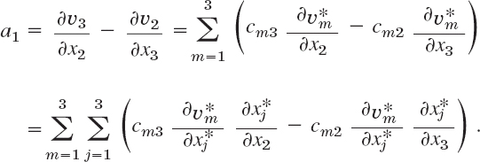
From this and (7) we obtain

Note what we did. The double sum had 3 × 3 = 9 terms, 3 of which were zero (when m = j), and the remaining 6 terms we combined in pairs as we needed them in getting ![]() .
.
We now use (3), Lagrange's identity (see Formula (15) in Team Project 24 in Problem Set 9.3) and k* × j* −i* and k × j = −i. Then

Hence ![]() . This is of the form of the first formula in (2) in Theorem A, and the other two formulas of the form (2) are obtained similarly. This proves the theorem for right-handed systems. If the x1x2x3-coordinates are left-handed, then k × j = +i, but then there is a minus sign in front of the determinant in (1), Sec. 9.9.
. This is of the form of the first formula in (2) in Theorem A, and the other two formulas of the form (2) are obtained similarly. This proves the theorem for right-handed systems. If the x1x2x3-coordinates are left-handed, then k × j = +i, but then there is a minus sign in front of the determinant in (1), Sec. 9.9.
PROOF OF THEOREM 1, PART (b) We prove that if
![]()
with continuous F1, F2, F3in a domain D is independent of path in D, then F = grad f in D for some f; in components

We choose any fixed A: (x0, y0, z0) in D and any B: (x, y, z) in D and define f by

with any constant f0 and any path from A to B in D. Since A is fixed and we have independence of path, the integral depends only on the coordinates x, y, z, so that (3) defines a function f(x, y, z) in D. We show that F = grad f with this f, beginning with the first of the three relations (2′). Because of independence of path we may integrate from A to B1: (x1, y, z) and then parallel to the x-axis along the segment B1B in Fig. 562 with B1 chosen so that the whole segment lies in D. Then

We now take the partial derivative with respect to x on both sides. On the left we get δf/δx. We show that on the right we get F1. The derivative of the first integral is zero because A: (x0, y0, z0) and B1: (x1, y, z) do not depend on x. We consider the second integral. Since on the segment B1B, both y and z are constant, the terms F2dy* and F3dz * do not contribute to the derivative of the integral. The remaining part can be written as a definite integral,

Fig. 562. Proof of Theorem 1

Hence its partial derivative with respect to x is F1(x, y, z), and the first of the relations (2′) is proved. The other two formulas in (2) follow by the same argument.
THEOREM Reality of Eigenvalues
If p, q, r, and p′ in the Sturm–Liouville equation (1) of Sec. 11.5 are real-valued and continuous on the interval a ![]() x
x ![]() b and r (x) > 0 throughout that interval (or r (x) 0 throughout that interval), then all the eigenvalues of the Sturm–Liouville problem (1), (2), Sec. 11.5, are real.
b and r (x) > 0 throughout that interval (or r (x) 0 throughout that interval), then all the eigenvalues of the Sturm–Liouville problem (1), (2), Sec. 11.5, are real.
PROOF
Let λ = α + iβ be an eigenvalue of the problem and let
![]()
be a corresponding eigenfunction; here α, β, u, and v are real. Substituting this into (1), Sec. 11.5, we have
![]()
This complex equation is equivalent to the following pair of equations for the real and the imaginary parts:
Multiplying the first equation by v, the second by −u and adding, we get

The expression in brackets is continuous on a ![]() x
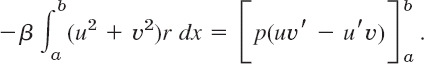
x ![]() b, for reasons similar to those in the proof of Theorem 1, Sec. 11.5. Integrating over x from a to b, we thus obtain
b, for reasons similar to those in the proof of Theorem 1, Sec. 11.5. Integrating over x from a to b, we thus obtain
Because of the boundary conditions, the right side is zero; this is as in that proof. Since y is an eigenfunction, u2 + v2 ![]() 0. Since y and r are continuous and r > (or r < 0) on the interval a
0. Since y and r are continuous and r > (or r < 0) on the interval a ![]() x
x ![]() b, the integral on the left is not zero. Hence, β = 0, which means that λ = α is real. This completes the proof.
b, the integral on the left is not zero. Hence, β = 0, which means that λ = α is real. This completes the proof.
PROOF OF THEOREM 2 Cauchy–Riemann Equations
We prove that Cauchy–Riemann equations
![]()
are sufficient for a complex function f(z) = u (x, y) + iv (x, y) to be analytic; precisely, if the real part u and the imaginary part v of f(z) satisfy (1) in a domain D in the complex plane and if the partial derivatives in (1) are continuous in D, then f(z) is analytic in D.
In this proof we write Δz = Δx + iΔy and Δf = f(z + Δz) − f(z). The idea of proof is as follows.
(a) We express Δf in terms of first partial derivatives of u and v, by applying the mean value theorem of Sec. 9.6.
(b) We get rid of partial derivatives with respect to y by applying the Cauchy–Riemann equations.
(c) We let Δz approach zero and show that then Δf/Δz, as obtained, approaches a limit, which is equal to ux + ivx, the right side of (4) in Sec. 13.4, regardless of the way of approach to zero.
(a) Let P: (x, y) be any fixed point in D. Since D is a domain, it contains a neighborhood of P. We can choose a point Q: (x + Δx, y + Δy) in this neighborhood such that the straight-line segment PQ is in D. Because of our continuity assumptions we may apply the mean value theorem in Sec. 9.6. This yields

where M1 and M2 (≠ M1 in general!) are suitable points on that segment. The first line is Re Δf and the second is Im Δf, so that
![]()
(b) uy = −vx and vy = ux by the Cauchy–Riemann equations, so that
![]()
Also Δz = Δx + iΔy, so that we can write Δx = Δz −iΔy in the first term and Δy = (Δz − Δx)/i = −i (Δz − Δx) in the second term. This gives
![]()
By performing the multiplications and reordering we obtain


(c) We finally let Δz approach zero and note that |Δy/Δz| ![]() 1 and |Δx/Δz|
1 and |Δx/Δz| ![]() 1 in (A). Then Q: (x + Δx, y + Δy) approaches P: (x, y), so that M1 and M2 must approach P. Also, since the partial derivatives in (A) are assumed to be continuous, they approach their value at P. In particular, the differences in the braces {…} in (A) approach zero. Hence the limit of the right side of (A) exists and is independent of the path along which Δz → 0. We see that this limit equals the right side of (4) in Sec. 13.4. This means that f(z) is analytic at every point z in D, and the proof is complete.
1 in (A). Then Q: (x + Δx, y + Δy) approaches P: (x, y), so that M1 and M2 must approach P. Also, since the partial derivatives in (A) are assumed to be continuous, they approach their value at P. In particular, the differences in the braces {…} in (A) approach zero. Hence the limit of the right side of (A) exists and is independent of the path along which Δz → 0. We see that this limit equals the right side of (4) in Sec. 13.4. This means that f(z) is analytic at every point z in D, and the proof is complete.
Section 14.2, pages 653–654
GOURSAT'S PROOF OF CAUCHY'S INTEGRAL THEOREM
Goursat proved Cauchy's integral theorem without assuming that f′(z) is continuous, as follows.
We start with the case when C is the boundary of a triangle. We orient C counterclockwise. By joining the midpoints of the sides we subdivide the triangle into four congruent triangles (Fig. 563). Let CI, CII, CIII, CIV denote their boundaries. We claim that (see Fig. 563).
![]()
Indeed, on the right we integrate along each of the three segments of subdivision in both possible directions (Fig. 563), so that the corresponding integrals cancel out in pairs, and the sum of the integrals on the right equals the integral on the left. We now pick an integral on the right that is biggest in absolute value and call its path C1. Then, by the triangle inequality (Sec. 13.2),
![]()
We now subdivide the triangle bounded by C1 as before and select a triangle of subdivision with boundary C2 for which

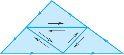
Fig. 563. Proof of Cauchy's integral theorem
Continuing in this fashion, we obtain a sequence of triangles T1, T2, … with boundaries C1, C2, … that are similar and such that Tn lies in Tm when n > m, and

Let z0 be the point that belongs to all these triangles. Since f is differentiable at z = z0, the derivative f′(z0) exists. Let

Solving this algebraically for f(z) we have
![]()
Integrating this over the boundary Cn of the triangle Tn gives
![]()
Since f(z0) and f′(z0) are constants and Cn is a closed path, the first two integrals on the right are zero, as follows from Cauchy's proof, which is applicable because the integrands do have continuous derivatives (0 and const, respectively). We thus have

Since f′(z0) is the limit of the difference quotient in (3), for given ![]() > 0 we can find a δ > 0 such that
> 0 we can find a δ > 0 such that
![]()
We may now take n so large that the triangle Tn lies in the disk |z − z0|< δ. Let Ln be the length of Cn. Then |z − z0| < Ln for all z on Cn and z0 in Tn. From this and (4) we have |h(z)(z − z0)| < ![]() Ln. The ML-inequality in Sec. 14.1 now gives
Ln. The ML-inequality in Sec. 14.1 now gives

Now denote the length of C by L. Then the path C1 has the length L1 = L/2, the path C2 has the length L2 = L1/2 = L/4, etc., and Cn has the length Ln = L/2n. Hence ![]() . From (2) and (5) we thus obtain
. From (2) and (5) we thus obtain

By choosing ![]() (> 0) sufficiently small we can make the expression on the right as small as we please, while the expression on the left is the definite value of an integral. Consequently, this value must be zero, and the proof is complete.
(> 0) sufficiently small we can make the expression on the right as small as we please, while the expression on the left is the definite value of an integral. Consequently, this value must be zero, and the proof is complete.
The proof for the case in which C is the boundary of a polygon follows from the previous proof by subdividing the polygon into triangles (Fig. 564). The integral corresponding to each such triangle is zero. The sum of these integrals is equal to the integral over C, because we integrate along each segment of subdivision in both directions, the corresponding integrals cancel out in pairs, and we are left with the integral over C.
The case of a general simple closed path C can be reduced to the preceding one by inscribing in C a closed polygon P of chords, which approximates C “sufficiently accurately,” and it can be shown that there is a polygon P such that the integral over P differs from that over C by less than any preassigned positive real number ![]() , no matter how small. The details of this proof are somewhat involved and can be found in Ref. [D6] listed in App. 1.
, no matter how small. The details of this proof are somewhat involved and can be found in Ref. [D6] listed in App. 1.
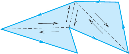
Fig. 564. Proof of Cauchy's integral theorem for a polygon
PROOF OF THEOREM 4 Cauchy's Convergence Principle for Series
(a) In this proof we need two concepts and a theorem, which we list first.
1. A bounded sequence s1, s2, … is a sequence whose terms all lie in a disk of (sufficiently large, finite) radius K with center at the origin; thus |sn| < K for all n.
2. A limit point a of a sequence s1, s2, … is a point such that, given an ![]() > 0, there are infinitely many terms satisfying |sn − a| >
> 0, there are infinitely many terms satisfying |sn − a| > ![]() . (Note that this does not imply convergence, since there may still be infinitely many terms that do not lie within that circle of radius and center a.)
. (Note that this does not imply convergence, since there may still be infinitely many terms that do not lie within that circle of radius and center a.)
![]()
3. A bounded sequence in the complex plane has at least one limit point. (Bolzano–Weierstrass theorem; proof below. Recall that “sequence” always means infinite sequence.)
(b) We now turn to the actual proof that z1 + z2 + … converges if and only if, for every ![]() > 0, we can find an N such that
> 0, we can find an N such that
![]()
Here, by the definition of partial sums,
![]()
Writing n + p = r, we see from this that (1) is equivalent to
![]()
Suppose that s1, s2, … converges. Denote its limit by s. Then for a given ![]() > 0 we can find an N such that
> 0 we can find an N such that
![]()
Hence, if r > N and n > N, then by the triangle inequality (Sec. 13.2),
![]()
that is, (1*) holds.
(c) Conversely, assume that s1, s2, … satisfies (1*). We first prove that then the sequence must be bounded. Indeed, choose a fixed and a fixed n = n0 > N in (1*). Then (1*) implies that all sr with r > N lie in the disk of radius ![]() and center sn0 and only finitely many terms s1, …, sN may not lie in this disk. Clearly, we can now find a circle so large that this disk and these finitely many terms all lie within this new circle. Hence the sequence is bounded. By the Bolzano–Weierstrass theorem, it has at least one limit point, call it s.
and center sn0 and only finitely many terms s1, …, sN may not lie in this disk. Clearly, we can now find a circle so large that this disk and these finitely many terms all lie within this new circle. Hence the sequence is bounded. By the Bolzano–Weierstrass theorem, it has at least one limit point, call it s.
We now show that the sequence is convergent with the limit s. Let ![]() > 0 be given. Then there is an N* such that |sr − sn|<
> 0 be given. Then there is an N* such that |sr − sn|<![]() /2 for all r > N* and n > N*, by (1*). Also, by the definition of a limit point, |sn − s| <
/2 for all r > N* and n > N*, by (1*). Also, by the definition of a limit point, |sn − s| < ![]() /2 for infinitely many n, so that we can find and fix an n > N* such that |sn − s|/2. Together, for every r > N *,
/2 for infinitely many n, so that we can find and fix an n > N* such that |sn − s|/2. Together, for every r > N *,
![]()
that is, the sequence s1, s2, … is convergent with the limit s.
THEOREM Bolzano–Weierstrass Theorem3
A bounded infinite sequence z1, z2, z3, … in the complex plane has at least one limit point.
PROOF
It is obvious that we need both conditions: a finite sequence cannot have a limit point, and the sequence 1, 2, 3, …, which is infinite but not bounded, has no limit point. To prove the theorem, consider a bounded infinite sequence z1, z2, … and let K be such that |zn| < K for all n. If only finitely many values of the zn are different, then, since the sequence is infinite, some number z must occur infinitely many times in the sequence, and, by definition, this number is a limit point of the sequence.
We may now turn to the case when the sequence contains infinitely many different terms. We draw a large square Q0 that contains all zn. We subdivide Q0 into four congruent squares, which we number 1, 2, 3, 4. Clearly, at least one of these squares (each taken with its complete boundary) must contain infinitely many terms of the sequence. The square of this type with the lowest number (1, 2, 3, or 4) will be denoted by Q1. This is the first step. In the next step we subdivide Q1 into four congruent squares and select a square Q2 by the same rule, and so on. This yields an infinite sequence of squares Q0, Q1, Q2, …, Qn, … with the property that the side of Qn approaches zero as n approaches infinity, and Qm contains all Qn with n > m. It is not difficult to see that the number which belongs to all these squares,4 call it z = a, is a limit point of the sequence. In fact, given an ![]() > 0, we can choose an N so large that the side of the square QN is less than
> 0, we can choose an N so large that the side of the square QN is less than ![]() and, since QN contains infinitely many zn, we have |zn − a| <
and, since QN contains infinitely many zn, we have |zn − a| < ![]() for infinitely many n. This completes the proof.
for infinitely many n. This completes the proof.
PART (b) OF THE PROOF OF THEOREM 5
We have to show that
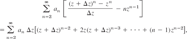
thus,
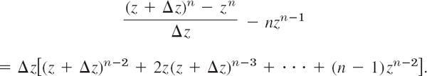
If we set z + Δz = b and z = a, thus Δz = b − a, this becomes simply
![]()
where An is the expression in the brackets on the right,
![]()
thus, A2 = 1, A3 = b + 2a, etc. We prove (7) by induction. When n = 2, then (7) holds, since then

Assuming that (7) holds for n = k, we show that it holds for n = k + 1. By adding and subtracting a term in the numerator and then dividing we first obtain

By the induction hypothesis, the right side equals b[(b − a)Ak + kak−1] + ak. Direct calculation shows that this is equal to
![]()
From (7b) with n = k we see that the expression in the braces {…} equals
![]()
Hence our result is

Taking the last term to the left, we obtain (7) with n = k + 1. This proves (7) for any integer n ![]() 2 and completes the proof.
2 and completes the proof.
ANOTHER PROOF OF THEOREM 1 without the use of a harmonic conjugate
We show that if w = u + iv = f(z) is analytic and maps a domain D conformally onto a domain D* and Φ*(u, v) is harmonic in D*, then
![]()
is harmonic in D, that is, ∇2Φ = 0 in D. We make no use of a harmonic conjugate of Φ*, but use straightforward differentiation. By the chain rule,
![]()
We apply the chain rule again, underscoring the terms that will drop out when we form ∇2Φ:

![]()
which is 0 by the Cauchy–Riemann equations. Also ∇2u = 0 and ∇2v = 0. There remains
![]()
By the Cauchy–Riemann equations this becomes
![]()
and is 0 since Φ* is harmonic.
1This proof was suggested by my colleague, Prof. A. D. Ziebur. In this proof, we use some formula numbers that have not yet been used in Sec. 2.6.
2LEOPOLD KRONECKER (1823–1891), German mathematician at Berlin, who made important contributions to algebra, group theory, and number theory.
We shall keep our discussion completely independent of Chap. 7, but readers familiar with matrices should recognize that we are dealing with orthogonal transformations and matrices and that our present theorem follows from Theorem 2 in Sec. 8.3.
3BERNARD BOLZANO (1781–1848), Austrian mathematician and professor of religious studies, was a pioneer in the study of point sets, the foundation of analysis, and mathematical logic.
For Weierstrass, see Sec. 15.5.
4 The fact that such a unique number z a exists seems to be obvious, but it actually follows from an axiom of the real number system, the so-called Cantor–Dedekind axiom: see footnote 3 in App. A3.3.