
APPENDIX 3
Auxiliary Material
A3.1 Formulas for Special Functions
For tables of numeric values, see Appendix 5.
Exponential function ex (Fig. 545)
Natural logarithm (Fig. 546)
![]()
ln x is the inverse of ex, and elnx = x, e−ln x = eln (1/x) = 1/x.
Logarithm of base ten log10x or simply log x

log x is the inverse of 10x, and 10logx = x, 10−log x = 1/x.
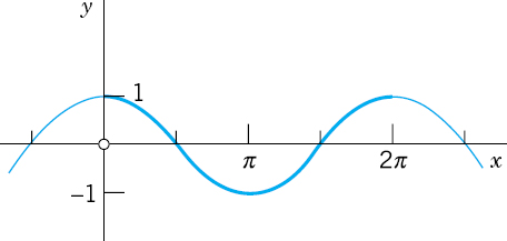
Sine and cosine functions (Figs. 547, 548). In calculus, angles are measured in radians, so that sin x and cos x have period 2π.
sin x is odd, sin (−x) = −sin x, and cos x is even, cos (−x) = cos x.

Fig. 545. Exponential function ex

Fig. 546. Natural logarithm ln x


Tangent, cotangent, secant, cosecant (Figs. 549, 550)

Hyperbolic functions (hyperbolic sine sinh x, etc.; Figs. 551, 552)
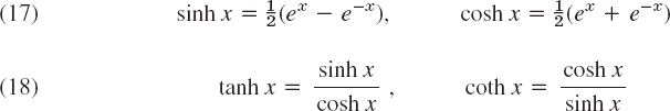

Fig. 551. sinh x (dashed) and cosh x

Fig. 552. tanh x (dashed) and coth x
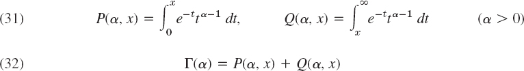
Gamma function (Fig. 553 and Table A2 in App. 5). The gamma function Γ(α) is defined by the integral

which is meaningful only if α > 0 (or, if we consider complex α, for those α whose real part is positive). Integration by parts gives the important functional relation of the gamma function,
![]()
From (24) we readily have Γ(1) = 1; hence if α is a positive integer, say k, then by repeated application of (25) we obtain
![]()
This shows that the gamma function can be regarded as a generalization of the elementary factorial function. [Sometimes the notation (α − 1)! is used for Γ(α), even for noninteger values of α, and the gamma function is also known as the factorial function.]
By repeated application of (25) we obtain
![]()
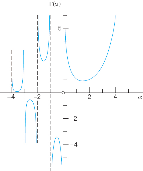

for defining the gamma function for negative α (≠ −1, −2, …), choosing for k the smallest integer such that α + k + 1 > 0. Together with (24), this then gives a definition of Γ(α) for all αnot equal to zero or a negative integer (Fig. 553).
It can be shown that the gamma function may also be represented as the limit of a product, namely, by the formula

From (27) or (28) we see that, for complex α, the gamma function Γ(α) is a meromorphic function with simple poles at α = 0, −1, −2, ….
An approximation of the gamma function for large positive α is given by the Stirling formula
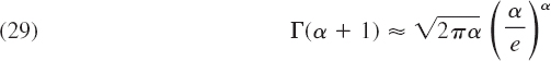
where e is the base of the natural logarithm. We finally mention the special value
![]()
Incomplete gamma functions
Beta function

Representation in terms of gamma functions:

Error function (Fig. 554 and Table A4 in App. 5)


erf (∞) = 1, complementary error function


![]() , complementary functions
, complementary functions

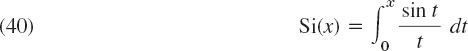
Sine integral (Fig. 556 and Table A4 in App. 5)


Si(∞) = π/2, complementary function

Cosine integral (Table A4 in App. 5)

Exponential integral

Logarithmic integral

A3.2 Partial Derivatives
For differentiation formulas, see inside of front cover.
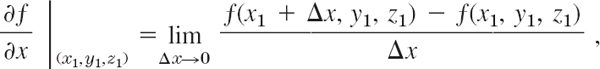
Let z = f(x, y) be a real function of two independent real variables, x and y. If we keep y constant, say, y = y1, and think of x as a variable, then f(x, y1) depends on x alone. If the derivative of f(x, y1) with respect to x for a value x = x1 exists, then the value of this derivative is called the partial derivative of f(x, y) with respect to x at the point (x1, y1) and is denoted by

Other notations are
![]()
these may be used when subscripts are not used for another purpose and there is no danger of confusion.
We thus have, by the definition of the derivative,

The partial derivative of z = f(x, y) with respect to y is defined similarly; we now keep x constant, say, equal to x1, and differentiate f(x1, y) with respect to y. Thus

Other notations are fy(x1, y1) and zy(x1, y1).
It is clear that the values of those two partial derivatives will in general depend on the point (x1, y1). Hence the partial derivatives ∂z/∂x and ∂z/∂y at a variable point (x, y) are functions of x and y. The function ∂z/∂x is obtained as in ordinary calculus by differentiating z = f(x, y) with respect to x, treating y as a constant, and ∂z/∂y is obtained by differentiating z with respect to y, treating x as a constant.

The partial derivatives ∂z/∂x and ∂z/∂y of a function z = f(x, y) have a very simple geometric interpretation. The function z = f(x, y) can be represented by a surface in space. The equation y =y1 then represents a vertical plane intersecting the surface in a curve, and the partial derivative ∂z/∂x at a point (x1, y1) is the slope of the tangent (that is, tan α where α is the angle shown in Fig. 557) to the curve. Similarly, the partial derivative ∂z/∂y at (x1, y1) is the slope of the tangent to the curve x = x1 on the surface z = f(x, y) at (x1, y1).
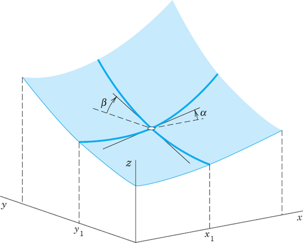
Fig. 557. Geometrical interpretation of first partial derivatives
The partial derivatives ∂z/∂x and ∂z/∂y are called first partial derivatives or partial derivatives of first order. By differentiating these derivatives once more, we obtain the four second partial derivatives (or partial derivatives of second order)2

It can be shown that if all the derivatives concerned are continuous, then the two mixed partial derivatives are equal, so that the order of differentiation does not matter (see Ref. [GenRef4] in App. 1), that is,

EXAMPLE 2 For the function in Example 1.
![]()
By differentiating the second partial derivatives again with respect to x and y, respectively, we obtain the third partial derivatives or partial derivatives of the third order of f, etc.
If we consider a function f(x, y, z) of three independent variables, then we have the three first partial derivatives fx(x, y, z), fy(x, y, z), and fz(x, y, z). Here fx is obtained by differentiating f with respect to x, treating both y and z as constants. Thus, analogous to (1), we now have
etc. By differentiating fx, fy, fz again in this fashion we obtain the second partial derivatives of f, etc.

A3.3 Sequences and Series
See also Chap. 15.
Monotone Real Sequences
We call a real sequence x1, x2, …, xn, … a monotone sequence if it is either monotone increasing, that is,
![]()
or monotone decreasing, that is,
![]()
We call x1, x2, … a bounded sequence if there is a positive constant K such that |xn| < K for all n.
PROOF
Let x1, x2, … be a bounded monotone increasing sequence. Then its terms are smaller than some number B and, since x1 ![]() xn for all n, they lie in the interval x1
xn for all n, they lie in the interval x1 ![]() xn
xn ![]() B, which will be denoted by I0. We bisect I0; that is, we subdivide it into two parts of equal length. If the right half (together with its endpoints) contains terms of the sequence, we denote it by I1. If it does not contain terms of the sequence, then the left half of I0 (together with its endpoints) is called I1. This is the first step.
B, which will be denoted by I0. We bisect I0; that is, we subdivide it into two parts of equal length. If the right half (together with its endpoints) contains terms of the sequence, we denote it by I1. If it does not contain terms of the sequence, then the left half of I0 (together with its endpoints) is called I1. This is the first step.
In the second step we bisect I1, select one half by the same rule, and call it I2, and so on (see Fig. 558).
In this way we obtain shorter and shorter intervals I0, I1, I2, … with the following properties. Each Im contains all In for n > m. No term of the sequence lies to the right of Im, and, since the sequence is monotone increasing, all xn with n greater than some number N lie in Im; of course, N will depend on m, in general. The lengths of the Im aapproach zero as m approaches infinity. Hence there is precisely one number, call it L, that lies in all those intervals,3 and we may now easily prove that the sequence is convergent with the limit L.
In fact, given an ![]() > 0, we choose an m such that the length of Im is less than
> 0, we choose an m such that the length of Im is less than ![]() . Then L and all the xn with n > N(m) lie in Im, and, therefore, |xn − L| <
. Then L and all the xn with n > N(m) lie in Im, and, therefore, |xn − L| < ![]() for all those n. This completes the proof for an increasing sequence. For a decreasing sequence the proof is the same, except for a suitable interchange of “left” and “right” in the construction of those intervals.
for all those n. This completes the proof for an increasing sequence. For a decreasing sequence the proof is the same, except for a suitable interchange of “left” and “right” in the construction of those intervals.

Fig. 558. Proof of Theorem 1
Real Series
THEOREM 2 Leibniz Test for Real Series
Let x1, x2, … be real and monotone decreasing to zero, that is,
![]()
Then the series with terms of alternating signs
![]()
converges, and for the remainder Rn after the nth term we have the estimate
![]()
PROOF
Let sn be the nth partial sum of the series. Then, because of (1a),
so that s2 ![]() s3
s3 ![]() s1. Proceeding in this fashion, we conclude that (Fig. 559)
s1. Proceeding in this fashion, we conclude that (Fig. 559)
![]()
which shows that the odd partial sums form a bounded monotone sequence, and so do the even partial sums. Hence, by Theorem 1, both sequences converge, say,
![]()

Fig. 559. Proof of the Leibniz test
Now, since s2n+1 − s2n = x2n+1, we readily see that (lb) implies
![]()
Hence s* = s, and the series converges with the sum s.
We prove the estimate (2) for the remainder. Since sn → s, it follows from (3) that
![]()
By subtracting s2n and s2n−1, respectively, we obtain
![]()
In these inequalities, the first expression is equal to x2n+1, the last is equal to −x2n, and the expressions between the inequality signs are the remainders R2n and R2n−1. Thus the inequalities may be written
![]()
and we see that they imply (2). This completes the proof.
A3.4 Grad, Div, Curl, ∇2
in Curvilinear Coordinates
To simplify formulas, we write Cartesian coordinates x = x1, y = x2, z = x3. We denote curvilinear coordinates by q1, q2, q3. Through each point P there pass three coordinate surfaces q1 = const, q2 = const, q3 = const. They intersect along coordinate curves. We assume the three coordinate curves through P to be orthogonal (perpendicular to each other). We write coordinate transformations as
![]()
Corresponding transformations of grad, div, curl, and ∇2 can all be written by using

Next to Cartesian coordinates, most important are cylindrical coordinates q1 = r, q2 = θ, q3 = z (Fig. 560a) defined by
![]()
and spherical coordinates q1 = r, q2 = θ, q3 = φ (Fig. 560b) defined by4


Fig. 560. Special curvilinear coordinates
In addition to the general formulas for any orthogonal coordinates q1, q2, q3, we shall give additional formulas for these important special cases.
Linear Elementds. In Cartesian coordinates,
![]()
For the q-coordinates,

For polar coordinates set dz2 = 0.
![]()
Gradient. grad ![]() (partial derivatives; Sec. 9.7). In the q-system, with u, v, w denoting unit vectors in the positive directions of the q1, q2, q3 coordinate curves, respectively,
(partial derivatives; Sec. 9.7). In the q-system, with u, v, w denoting unit vectors in the positive directions of the q1, q2, q3 coordinate curves, respectively,

Divergence div F = ∇·F = (F1)x1 + (F2)x2 + (F3)x3 (F = [F1, F2, F3], Sec. 9.8);


Laplacian ![]() (Sec. 9.8):
(Sec. 9.8):

Curl (Sec. 9.9):
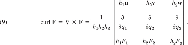
For cylindrical coordinates we have in (9) (as in the previous formulas)
![]()
and for spherical coordinates we have
![]()
1AUGUSTIN FRESNEL (1788–1827), French physicist and mathematician. For tables see Ref. [GenRef1].
2CAUTION! In the subscript notation, the subscripts are written in the order in which we differentiate, whereas in the “∂” notation the order is opposite.
3This statement seems to be obvious, but actually it is not; it may be regarded as an axiom of the real number system in the following form. Let J1, J2, … be closed intervals such that each Jm contains all Jn with n >m, and the lengths of the Jm approach zero as m approaches infinity. Then there is precisely one real number that is contained in all those intervals. This is the so-called Cantor–Dedekind axiom, named after the German mathematicians GEORG CANTOR (1845–1918), the creator of set theory, and RICHARD DEDEKIND (1831–1916), known for his fundamental work in number theory. For further details see Ref. [GenRef2] in App. 1. (An interval I is said to be closed if its two endpoints are regarded as points belonging to I. It is said to be open if the endpoints are not regarded as points of I.)
4This is the notation used in calculus and in many other books. It is logical since in it, θ plays the same role as in polar coordinates. CAUTION! Some books interchange the roles of θ and φ.