
CHAPTER 7
Linear Algebra: Matrices, Vectors, Determinants. Linear Systems
Linear algebra is a fairly extensive subject that covers vectors and matrices, determinants, systems of linear equations, vector spaces and linear transformations, eigenvalue problems, and other topics. As an area of study it has a broad appeal in that it has many applications in engineering, physics, geometry, computer science, economics, and other areas. It also contributes to a deeper understanding of mathematics itself.
Matrices, which are rectangular arrays of numbers or functions, and vectors are the main tools of linear algebra. Matrices are important because they let us express large amounts of data and functions in an organized and concise form. Furthermore, since matrices are single objects, we denote them by single letters and calculate with them directly. All these features have made matrices and vectors very popular for expressing scientific and mathematical ideas.
The chapter keeps a good mix between applications (electric networks, Markov processes, traffic flow, etc.) and theory. Chapter 7 is structured as follows: Sections 7.1 and 7.2 provide an intuitive introduction to matrices and vectors and their operations, including matrix multiplication. The next block of sections, that is, Secs. 7.3–7.5 provide the most important method for solving systems of linear equations by the Gauss elimination method. This method is a cornerstone of linear algebra, and the method itself and variants of it appear in different areas of mathematics and in many applications. It leads to a consideration of the behavior of solutions and concepts such as rank of a matrix, linear independence, and bases. We shift to determinants, a topic that has declined in importance, in Secs. 7.6 and 7.7. Section 7.8 covers inverses of matrices. The chapter ends with vector spaces, inner product spaces, linear transformations, and composition of linear transformations. Eigenvalue problems follow in Chap. 8.
COMMENT. Numeric linear algebra (Secs. 20.1–20.5) can be studied immediately after this chapter.
Prerequisite: None.
Sections that may be omitted in a short course: 7.5, 7.9.
References and Answers to Problems: App. 1 Part B, and App. 2.
7.1 Matrices, Vectors: Addition and Scalar Multiplication
The basic concepts and rules of matrix and vector algebra are introduced in Secs. 7.1 and 7.2 and are followed by linear systems (systems of linear equations), a main application, in Sec. 7.3.
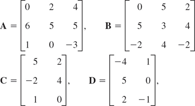
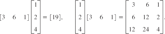
Let us first take a leisurely look at matrices before we formalize our discussion. A matrix is a rectangular array of numbers or functions which we will enclose in brackets. For example,

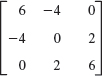
are matrices. The numbers (or functions) are called entries or, less commonly, elements of the matrix. The first matrix in (1) has two rows, which are the horizontal lines of entries. Furthermore, it has three columns, which are the vertical lines of entries. The second and third matrices are square matrices, which means that each has as many rows as columns—3 and 2, respectively. The entries of the second matrix have two indices, signifying their location within the matrix. The first index is the number of the row and the second is the number of the column, so that together the entry's position is uniquely identified. For example, a23 (read a two three) is in Row 2 and Column 3, etc. The notation is standard and applies to all matrices, including those that are not square.
Matrices having just a single row or column are called vectors. Thus, the fourth matrix in (1) has just one row and is called a row vector. The last matrix in (1) has just one column and is called a column vector. Because the goal of the indexing of entries was to uniquely identify the position of an element within a matrix, one index suffices for vectors, whether they are row or column vectors. Thus, the third entry of the row vector in (1) is denoted by a3.
Matrices are handy for storing and processing data in applications. Consider the following two common examples.
EXAMPLE 1 Linear Systems, a Major Application of Matrices
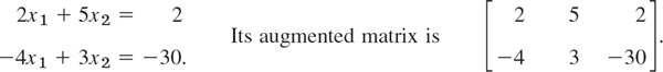
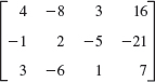
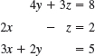
We are given a system of linear equations, briefly a linear system, such as

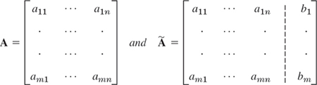
where x1, x2, x3 are the unknowns. We form the coefficient matrix, call it A, by listing the coefficients of the unknowns in the position in which they appear in the linear equations. In the second equation, there is no unknown x2, which means that the coefficient of x2 is 0 and hence in matrix A, a22 = 0, Thus,
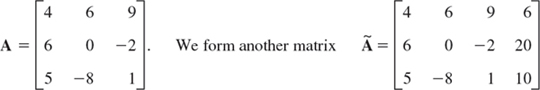
by augmenting A with the right sides of the linear system and call it the augmented matrix of the system.
Since we can go back and recapture the system of linear equations directly from the augmented matrix Ã, Ã contains all the information of the system and can thus be used to solve the linear system. This means that we can just use the augmented matrix to do the calculations needed to solve the system. We shall explain this in detail in Sec. 7.3. Meanwhile you may verify by substitution that the solution is ![]() .
.
The notation x1, x2, x3 for the unknowns is practical but not essential; we could choose x, y, z or some other letters.
EXAMPLE 2 Sales Figures in Matrix Form
Sales figures for three products I, II, III in a store on Monday (Mon), Tuesday (Tues), may for each week be arranged in a matrix

If the company has 10 stores, we can set up 10 such matrices, one for each store. Then, by adding corresponding entries of these matrices, we can get a matrix showing the total sales of each product on each day. Can you think of other data which can be stored in matrix form? For instance, in transportation or storage problems? Or in listing distances in a network of roads?
General Concepts and Notations
Let us formalize what we just have discussed. We shall denote matrices by capital boldface letters A, B, C, …, or by writing the general entry in brackets; thus A = [ajk], and so on. By an m × n matrix (read m by n matrix) we mean a matrix with m rows and n columns—rows always come first! m × n is called the size of the matrix. Thus an m × n matrix is of the form

The matrices in (1) are of sizes 2 × 3, 3 × 3, 2 × 2, 1 × 3, and 2 × 1, respectively.
Each entry in (2) has two subscripts. The first is the row number and the second is the column number. Thus a21 is the entry in Row 2 and Column 1.
If m = n we call A an n × n square matrix. Then its diagonal containing the entries a11, a22, …, ann is called the main diagonal of A. Thus the main diagonals of the two square matrices in (1) are a11, a22, a33 and e−x, 4x, respectively.
Square matrices are particularly important, as we shall see. A matrix of any size m × n is called a rectangular matrix; this includes square matrices as a special case.
Vectors
A vector is a matrix with only one row or column. Its entries are called the components of the vector. We shall denote vectors by lowercase boldface letters a, b, … or by its general component in brackets, a = [aj], and so on. Our special vectors in (1) suggest that a (general) row vector is of the form
![]()
A column vector is of the form

Addition and Scalar Multiplication of Matrices and Vectors
What makes matrices and vectors really useful and particularly suitable for computers is the fact that we can calculate with them almost as easily as with numbers. Indeed, we now introduce rules for addition and for scalar multiplication (multiplication by numbers) that were suggested by practical applications. (Multiplication of matrices by matrices follows in the next section.) We first need the concept of equality.
DEFINITION Equality of Matrices
Two matrices A = [ajk] and B = [bjk] are equal, written A = B, if and only if they have the same size and the corresponding entries are equal, that is, a11 = b11, and a12 = b12, so on. Matrices that are not equal are called different. Thus, matrices of different sizes are always different.


DEFINITION Addition of Matrices
The sum of two matrices A = [ajk] and B = [bjk] of the same size is written A + B and has the entries ajk + bjk obtained by adding the corresponding entries of A and B. Matrices of different sizes cannot be added.
As a special case, the sum a + b of two row vectors or two column vectors, which must have the same number of components, is obtained by adding the corresponding components.
EXAMPLE 4 Addition of Matrices and Vectors

A in Example 3 and our present A cannot be added. If a = [5 7 2] and b = [−6 2 0], then a + b = [−1 9 2].
An application of matrix addition was suggested in Example 2. Many others will follow.
DEFINITION Scalar Multiplication (Multiplication by a Number)
The product of any m × n matrix A = [ajk] and any scalar c (number c) is written cA and is the m × n matrix cA = [cajk] obtained by multiplying each entry of A by c.
Here (−1)A is simply written −A and is called the negative of A. Similarly, (−k)A is written −kA. Also, A + (−B) is written A − B and is called the difference of A and B (which must have the same size!).
EXAMPLE 5 Scalar Multiplication
If a matrix B shows the distances between some cities in miles, 1.609B gives these distances in kilometers.
Rules for Matrix Addition and Scalar Multiplication. From the familiar laws for the addition of numbers we obtain similar laws for the addition of matrices of the same size m × n, namely,

Here 0 denotes the zero matrix (of size m × n), that is, the m × n matrix with all entries zero. If m = 1 or n = 1, this is a vector, called a zero vector.
Hence matrix addition is commutative and associative [by (3a) and (3b)]. Similarly, for scalar multiplication we obtain the rules

1–7 GENERAL QUESTIONS
- Equality. Give reasons why the five matrices in Example 3 are all different.
- Double subscript notation. If you write the matrix in Example 2 in the form A = [ajk], what is a31? a13? a26? a33?
- Sizes. What sizes do the matrices in Examples 1, 2, 3, and 5 have?
- Main diagonal. What is the main diagonal of A in Example 1? Of A and B in Example 3?
- Scalar multiplication. If A in Example 2 shows the number of items sold, what is the matrix B of units sold if a unit consists of (a) 5 items and (b) 10 items?
- If a 12 × 12 matrix A shows the distances between 12 cities in kilometers, how can you obtain from A the matrix B showing these distances in miles?
- Addition of vectors. Can you add: A row and a column vector with different numbers of components? With the same number of components? Two row vectors with the same number of components but different numbers of zeros? A vector and a scalar? A vector with four components and a 2 × 2 matrix?
8–16 ADDITION AND SCALAR MULTIPLICATION OF MATRICES AND VECTORS
Let

Find the following expressions, indicating which of the rules in (3) or (4) they illustrate, or give reasons why they are not defined.
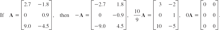
- 8. 2A + 4B, 4B + 2A, 0A + B, 0.4B − 4.2A
- 9. 3A, 0.5B, 3A + 0.5B, 3A + 0.5B + C
- 10. (4 · 3)A, 4(3A), 14B − 3B, 11B
- 11. 8C + 10D, 2(5D + 4C), 0.6C − 0.6D, 0.6(C − D)
- 12. (C + D) + E, (D + E) + C, 0(C − E) + 4D, A − 0C
- 13. (2 · 7)C, 2(7C), −D + 0E, E − D + C + u
- 14.

- 15. (u + v) − w, u + (v − w), C + 0w, 0E + u − v
- 16. 15v − 3w − 0u, −3w + 15v, D − u + 3C, 8.5w − 11.1u + 0.4v
- 17. Resultant of forces. If the above vectors u, v, w represent forces in space, their sum is called their resultant. Calculate it.
- 18. Equilibrium. By definition, forces are in equilibrium if their resultant is the zero vector. Find a force p such that the above u, v, w, and p are in equilibrium.
- 19. General rules. Prove (3) and (4) for general 2 × 3 matrices and scalars c and k.
- 20. TEAM PROJECT. Matrices for Networks. Matrices have various engineering applications, as we shall see. For instance, they can be used to characterize connections in electrical networks, in nets of roads, in production processes, etc., as follows.
(a) Nodal Incidence Matrix. The network in Fig. 155 consists of six branches (connections) and four nodes (points where two or more branches come together). One node is the reference node (grounded node, whose voltage is zero). We number the other nodes and number and direct the branches. This we do arbitrarily. The network can now be described by a matrix A = [ajk], where

A is called the nodal incidence matrix of the network. Show that for the network in Fig. 155 the matrix A has the given form.

Fig. 155. Network and nodal incidence matrix in Team Project 20(a)
(b) Find the nodal incidence matrices of the networks in Fig. 156.
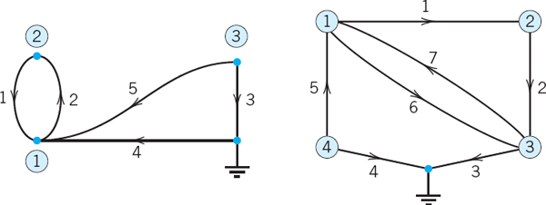
Fig. 156. Electrical networks in Team Project 20(b)
(c) Sketch the three networks corresponding to the nodal incidence matrices

(d) Mesh Incidence Matrix. A network can also be characterized by the mesh incidence matrix M = [mjk], where
and a mesh is a loop with no branch in its interior (or in its exterior). Here, the meshes are numbered and directed (oriented) in an arbitrary fashion. Show that for the network in Fig. 157, the matrix M has the given form, where Row 1 corresponds to mesh 1, etc.

7.2 Matrix Multiplication
Matrix multiplication means that one multiplies matrices by matrices. Its definition is standard but it looks artificial. Thus you have to study matrix multiplication carefully, multiply a few matrices together for practice until you can understand how to do it. Here then is the definition. (Motivation follows later.)
DEFINITION Multiplication of a Matrix by a Matrix
The product C = AB (in this order) of an m × n matrix A = [ajk] times an r × p matrix B = [bjk] is defined if and only if r = n and is then the m × p matrix C = [cjk] with entries
The condition r = n means that the second factor, B, must have as many rows as the first factor has columns, namely n. A diagram of sizes that shows when matrix multiplication is possible is as follows:

The entry cjk in (1) is obtained by multiplying each entry in the jth row of A by the corresponding entry in the kth column of B and then adding these n products. For instance, c21 = a21b11 + a22b21 + … + a2nbn1, and so on. One calls this briefly a multiplication of rows into columns. For n = 3, this is illustrated by

where we shaded the entries that contribute to the calculation of entry c21 just discussed.
Matrix multiplication will be motivated by its use in linear transformations in this section and more fully in Sec. 7.9.
Let us illustrate the main points of matrix multiplication by some examples. Note that matrix multiplication also includes multiplying a matrix by a vector, since, after all, a vector is a special matrix.
EXAMPLE 1 Matrix Multiplication

Here c11 = 3 · 2 + 5 · 5 + (−1) · 9 = 22, and so on. The entry in the box is c23 = 4 · 3 + 0 · 7 + 2 · 1 = 14. The product BA is not defined.

EXAMPLE 4 CAUTION! Matrix Multiplication Is Not Commutative, AB ≠ BA in General
This is illustrated by Examples 1 and 2, where one of the two products is not even defined, and by Example 3, where the two products have different sizes. But it also holds for square matrices. For instance,

It is interesting that this also shows that AB = 0 does not necessarily imply BA = 0 or A = 0 or B = 0. We shall discuss this further in Sec. 7.8, along with reasons when this happens.
Our examples show that in matrix products the order of factors must always be observed very carefully. Otherwise matrix multiplication satisfies rules similar to those for numbers, namely.
provided A, B, and C are such that the expressions on the left are defined; here, k is any scalar. (2b) is called the associative law. (2c) and (2d) are called the distributive laws.
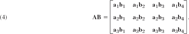
Since matrix multiplication is a multiplication of rows into columns, we can write the defining formula (1) more compactly as

where aj is the jth row vector of A and bk is the kth column vector of B, so that in agreement with (1),
EXAMPLE 5 Product in Terms of Row and Column Vectors
If A = [ajk] is of size 3 × 3 and B = [bjk] is of size 3 × 4, then
Taking a1 = [3 5 −1], a2 = [4 0 2], etc., verify (4) for the product in Example 1.
Parallel processing of products on the computer is facilitated by a variant of (3) for computing C = AB, which is used by standard algorithms (such as in Lapack). In this method, A is used as given, B is taken in terms of its column vectors, and the product is computed columnwise; thus,
![]()
Columns of B are then assigned to different processors (individually or several to each processor), which simultaneously compute the columns of the product matrix Ab1, Ab2, etc.
EXAMPLE 6 Computing Products Columnwise by (5)
To obtain

from (5), calculate the columns

of AB and then write them as a single matrix, as shown in the first formula on the right.
Motivation of Multiplication by Linear Transformations
Let us now motivate the “unnatural” matrix multiplication by its use in linear transformations. For n = 2 variables these transformations are of the form

and suffice to explain the idea. (For general n they will be discussed in Sec. 7.9.) For instance, (6*) may relate an x1x2-coordinate system to a y1y2-coordinate system in the plane. In vectorial form we can write (6*) as

Now suppose further that the x1x2-system is related to a w1w2-system by another linear transformation, say,
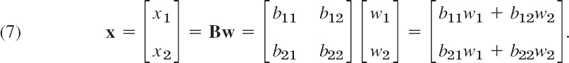
Then the y1y2-system is related to the w1w2-system indirectly via the x1x2-system, and we wish to express this relation directly. Substitution will show that this direct relation is a linear transformation, too, say,

Indeed, substituting (7) into (6), we obtain
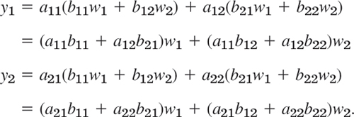
Comparing this with (8), we see that

This proves that C = AB with the product defined as in (1). For larger matrix sizes the idea and result are exactly the same. Only the number of variables changes. We then have m variables y and n variables x and p variables w. The matrices A, B, and C = AB then have sizes m × n, n × p, and m × p, respectively. And the requirement that C be the product AB leads to formula (1) in its general form. This motivates matrix multiplication.
Transposition
We obtain the transpose of a matrix by writing its rows as columns (or equivalently its columns as rows). This also applies to the transpose of vectors. Thus, a row vector becomes a column vector and vice versa. In addition, for square matrices, we can also “reflect” the elements along the main diagonal, that is, interchange entries that are symmetrically positioned with respect to the main diagonal to obtain the transpose. Hence a12 becomes a21, a31 becomes a13, and so forth. Example 7 illustrates these ideas. Also note that, if A is the given matrix, then we denote its transpose by AT.
EXAMPLE 7 Transposition of Matrices and Vectors

A little more compactly, we can write

Furthermore, the transpose [6 2 3]T of the row vector [6 2 3] is the column vector
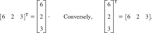
DEFINITION Transposition of Matrices and Vectors
The transpose of an m × n matrix A = [ajk] is the n × m matrix AT (read A transpose) that has the first row of A as its first column, the second row of A as its second column, and so on. Thus the transpose of A in (2) is AT = [akj], written out
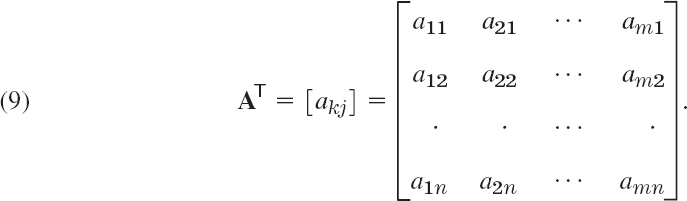
As a special case, transposition converts row vectors to column vectors and conversely.
Transposition gives us a choice in that we can work either with the matrix or its transpose, whichever is more convenient.
Rules for transposition are
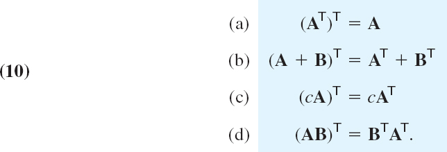
CAUTION! Note that in (10d) the transposed matrices are in reversed order. We leave the proofs as an exercise in Probs. 9 and 10.
Special Matrices
Certain kinds of matrices will occur quite frequently in our work, and we now list the most important ones of them.
Symmetric and Skew-Symmetric Matrices. Transposition gives rise to two useful classes of matrices. Symmetric matrices are square matrices whose transpose equals the matrix itself. Skew-symmetric matrices are square matrices whose transpose equals minus the matrix. Both cases are defined in (11) and illustrated by Example 8.

EXAMPLE 8 Symmetric and Skew-Symmetric Matrices
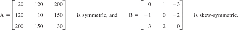
For instance, if a company has three building supply centers C1, C2, C3, then A could show costs, say, ajj for handling 1000 bags of cement at center Cj, and ajk(j ≠ k) the cost of shipping 1000 bags from Cj to Ck to. Clearly, ajk = akj if we assume shipping in the opposite direction will cost the same.
Symmetric matrices have several general properties which make them important. This will be seen as we proceed.
Triangular Matrices. Upper triangular matrices are square matrices that can have nonzero entries only on and above the main diagonal, whereas any entry below the diagonal must be zero. Similarly, lower triangular matrices can have nonzero entries only on and below the main diagonal. Any entry on the main diagonal of a triangular matrix may be zero or not.
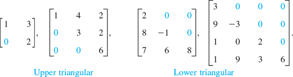
Diagonal Matrices. These are square matrices that can have nonzero entries only on the main diagonal. Any entry above or below the main diagonal must be zero.
If all the diagonal entries of a diagonal matrix S are equal, say, c, we call S a scalar matrix because multiplication of any square matrix A of the same size by S has the same effect as the multiplication by a scalar, that is,
![]()
In particular, a scalar matrix, whose entries on the main diagonal are all 1, is called a unit matrix (or identity matrix) and is denoted by In or simply by I. For I, formula (12) becomes
![]()

Some Applications of Matrix Multiplication
EXAMPLE 11 Computer Production. Matrix Times Matrix
Supercomp Ltd produces two computer models PC1086 and PC1186. The matrix A shows the cost per computer (in thousands of dollars) and B the production figures for the year 2010 (in multiples of 10,000 units.) Find a matrix C that shows the shareholders the cost per quarter (in millions of dollars) for raw material, labor, and miscellaneous.
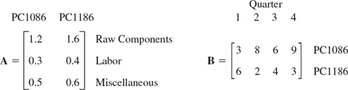
Solution.

Since cost is given in multiples of $1000 and production in multiples of 10,000 units, the entries of C are multiples of $10 millions; thus c11 = 13.2 means $132 million, etc.
EXAMPLE 12 Weight Watching. Matrix Times Vector
Suppose that in a weight-watching program, a person of 185 lb burns 350 cal/hr in walking (3 mph), 500 in bicycling (13 mph), and 950 in jogging (5.5 mph). Bill, weighing 185 lb, plans to exercise according to the matrix shown. Verify the calculations (W = Walking, B = Bicycling, J = Jogging).

EXAMPLE 13 Markov Process. Powers of a Matrix. Stochastic Matrix
Suppose that the 2004 state of land use in a city of 60 mi2 of built-up area is
![]()
Find the states in 2009, 2014, and 2019, assuming that the transition probabilities for 5-year intervals are given by the matrix A and remain practically the same over the time considered.

A is a stochastic matrix, that is, a square matrix with all entries nonnegative and all column sums equal to 1. Our example concerns a Markov process,1 that is, a process for which the probability of entering a certain state depends only on the last state occupied (and the matrix A), not on any earlier state.
Solution. From the matrix A and the 2004 state we can compute the 2009 state,
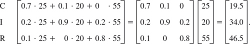
To explain: The 2009 figure for C equals times the probability 0.7 that C goes into C, plus times the probability 0.1 that I goes into C, plus times the probability 0 that R goes into C. Together,
![]()
Similarly, the new R is 46.5%. We see that the 2009 state vector is the column vector
![]()
where the column vector x = [25 20 55]T is the given 2004 state vector. Note that the sum of the entries of y is 100 [%]. Similarly, you may verify that for 2014 and 2019 we get the state vectors

Answer. In 2009 the commercial area will be 19.5% (11.7 mi2), the industrial 34% (20.4 mi2), and the residential 46.5% (27.9 mi2). For 2014 the corresponding figures are 17.05%, 43.80%, and 39.15%. For 2019 they are 16.315%, 50.660%, and 33.025%. (In Sec. 8.2 we shall see what happens in the limit, assuming that those probabilities remain the same. In the meantime, can you experiment or guess?)
1–10 GENERAL QUESTIONS
- Multiplication. Why is multiplication of matrices restricted by conditions on the factors?
- Square matrix. What form does a 3 × 3 matrix have if it is symmetric as well as skew-symmetric?
- Product of vectors. Can every 3 × 3 matrix be represented by two vectors as in Example 3?
- Skew-symmetric matrix. How many different entries can a 4 × 4 skew-symmetric matrix have? An n × n skew-symmetric matrix?
- Same questions as in Prob. 4 for symmetric matrices.
- Triangular matrix. If U1, U2 are upper triangular and L1, L2 are lower triangular, which of the following are triangular?

- Idempotent matrix, defined by A2 = A. Can you find four 2 × 2 idempotent matrices?
- Nilpotent matrix, defined by Bm = 0 for some m. Can you find three 2 × 2 nilpotent matrices?
- Transposition. Can you prove (10a)–(10c) for 3 × 3 matrices? For m × n matrices?
- Transposition. (a) Illustrate (10d) by simple examples. (b) Prove (10d).
11–20 MULTIPLICATION, ADDITION, AND TRANSPOSITION OF MATRICES AND VECTORS
Let

Showing all intermediate results, calculate the following expressions or give reasons why they are undefined:
- 11. AB, ABT, BA, BTA
- 12. AAT, A2, BBT, B2
- 13. CCT, BC, CD, CTB
- 14. 3A − 2B, (3A − 2B)T, 3AT − 2BT, (3A − 2B)TaT
- 15. Aa, AaT, (Ab)T, bTAT
- 16. BC, BCT, Bb, bTB
- 17. ABC, ABa, ABb, CaT
- 18. ab, ba, aA, Bb
- 19. 1.5a + 3.0b, 1.5aT + 3.0b, (A − B)b, Ab − Bb
- 20. bTAb, aBaT, aCCT, CTba
- 21. General rules. Prove (2) for 2 × 2 matrices A = [ajk], B = [bjk], C = [cjk], and a general scalar.
- 22. Product. Write AB in Prob. 11 in terms of row and column vectors.
- 23. Product. Calculate AB in Prob. 11 columnwise. See Example 1.
- 24. Commutativity. Find all 2 × 2 matrices A = [ajk] that commute with B = [bjk], where bjk = j + k.
- 25. TEAM PROJECT. Symmetric and Skew-Symmetric Matrices. These matrices occur quite frequently in applications, so it is worthwhile to study some of their most important properties.
(a) Verify the claims in (11) that akj = ajk for a symmetric matrix, and akj = −ajk for a skew-symmetric matrix. Give examples.
(b) Show that for every square matrix C the matrix C + CT is symmetric and C − CT is skew-symmetric. Write C in the form C = S + T, where S is symmetric and T is skew-symmetric and find S and T in terms of C. Represent A and B in Probs. 11–20 in this form.
(c) A linear combination of matrices A, B, C, …, M of the same size is an expression of the form

where a, …, m are any scalars. Show that if these matrices are square and symmetric, so is (14); similarly, if they are skew-symmetric, so is (14).
(d) Show that AB with symmetric A and B is symmetric if and only if A and B commute, that is, AB = BA.
(e) Under what condition is the product of skew-symmetric matrices skew-symmetric?
26–30 FURTHER APPLICATIONS
- 26. Production. In a production process, let N mean “no trouble” and T “trouble.” Let the transition probabilities from one day to the next be 0.8 for N → N, hence 0.2 for N → T, and 0.5 for T → N, hence 0.5 for T → T.
If today there is no trouble, what is the probability of N two days after today? Three days after today?
- 27. CAS Experiment. Markov Process. Write a program for a Markov process. Use it to calculate further steps in Example 13 of the text. Experiment with other stochastic 3 × 3 matrices, also using different starting values.
- 28. Concert subscription. In a community of 100,000 adults, subscribers to a concert series tend to renew their subscription with probability 90% and persons presently not subscribing will subscribe for the next season with probability 0.2%. If the present number of subscribers is 1200, can one predict an increase, decrease, or no change over each of the next three seasons?
- 29. Profit vector. Two factory outlets F1 and F2 in New York and Los Angeles sell sofas (S), chairs (C), and tables (T) with a profit of $35, $62, and $30, respectively. Let the sales in a certain week be given by the matrix

Introduce a “profit vector” p such that the components of v = Ap give the total profits of F1 and F2.
- 30. TEAM PROJECT. Special Linear Transformations. Rotations have various applications. We show in this project how they can be handled by matrices.
(a) Rotation in the plane. Show that the linear transformation y = Ax with

is a counterclockwise rotation of the Cartesian x1x2-coordinate system in the plane about the origin, where θ is the angle of rotation.
(b) Rotation through nθ. Show that in (a)

Is this plausible? Explain this in words.
(c) Addition formulas for cosine and sine. By geometry we should have

Derive from this the addition formulas (6) in App. A3.1.
(d) Computer graphics. To visualize a three-dimensional object with plane faces (e.g., a cube), we may store the position vectors of the vertices with respect to a suitable x1x2x3-coordinate system (and a list of the connecting edges) and then obtain a two-dimensional image on a video screen by projecting the object onto a coordinate plane, for instance, onto the x1x2-plane by setting x3 = 0. To change the appearance of the image, we can impose a linear transformation on the position vectors stored. Show that a diagonal matrix D with main diagonal entries 3, 1,
 gives from an x = [xj] the new position vector y = Dx, where y1 = 3x1 (stretch in the x1-direction by a factor 3), y2 = x2 (unchanged),
  (contraction in the x3-direction). What effect would a scalar matrix have?
(e) Rotations in space. Explain y = Ax geometrically when A is one of the three matrices

What effect would these transformations have in situations such as that described in (d)?
7.3 Linear Systems of Equations. Gauss Elimination
We now come to one of the most important use of matrices, that is, using matrices to solve systems of linear equations. We showed informally, in Example 1 of Sec. 7.1, how to represent the information contained in a system of linear equations by a matrix, called the augmented matrix. This matrix will then be used in solving the linear system of equations. Our approach to solving linear systems is called the Gauss elimination method. Since this method is so fundamental to linear algebra, the student should be alert.
A shorter term for systems of linear equations is just linear systems. Linear systems model many applications in engineering, economics, statistics, and many other areas. Electrical networks, traffic flow, and commodity markets may serve as specific examples of applications.
Linear System, Coefficient Matrix, Augmented Matrix
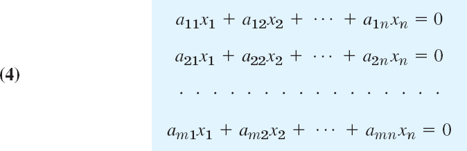
A linear system of m equations in n unknowns x1, …, xn is a set of equations of the form

The system is called linear because each variable xj appears in the first power only, just as in the equation of a straight line. a11, …, amn are given numbers, called the coefficients of the system. b1, …, bm on the right are also given numbers. If all the bj are zero, then (1) is called a homogeneous system. If at least one bj is not zero, then (1) is called a nonhomogeneous system.
A solution of (1) is a set of numbers x1, …, xn that satisfies all the m equations. A solution vector of (1) is a vector x whose components form a solution of (1). If the system (1) is homogeneous, it always has at least the trivial solution x1 = 0, …, xn = 0.
Matrix Form of the Linear System (1). From the definition of matrix multiplication we see that the m equations of (1) may be written as a single vector equation

where the coefficient matrix A = [ajk] is the m × n matrix

are column vectors. We assume that the coefficients ajk are not all zero, so that A is not a zero matrix. Note that x has n components, whereas b has m components. The matrix
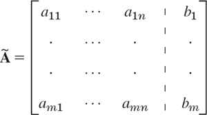
is called the augmented matrix of the system (1). The dashed vertical line could be omitted, as we shall do later. It is merely a reminder that the last column of à did not come from matrix A but came from vector b. Thus, we augmented the matrix A.
Note that the augmented matrix à determines the system (1) completely because it contains all the given numbers appearing in (1).
EXAMPLE 1 Geometric Interpretation. Existence and Uniqueness of Solutions
If m = n = 2, we have two equations in two unknowns x1, x2
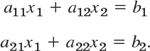
If we interpret x1, x2 as coordinates in the x1x2-plane, then each of the two equations represents a straight line, and (x1, x2) is a solution if and only if the point P with coordinates x1, x2 lies on both lines. Hence there are three possible cases (see Fig. 158 on next page):
- Precisely one solution if the lines intersect
- Infinitely many solutions if the lines coincide
- No solution if the lines are parallel

Fig. 158. Three equations in three unknowns interpreted as planes in space
If the system is homogenous, Case (c) cannot happen, because then those two straight lines pass through the origin, whose coordinates (0, 0) constitute the trivial solution. Similarly, our present discussion can be extended from two equations in two unknowns to three equations in three unknowns. We give the geometric interpretation of three possible cases concerning solutions in Fig. 158. Instead of straight lines we have planes and the solution depends on the positioning of these planes in space relative to each other. The student may wish to come up with some specific examples.
Our simple example illustrated that a system (1) may have no solution. This leads to such questions as: Does a given system (1) have a solution? Under what conditions does it have precisely one solution? If it has more than one solution, how can we characterize the set of all solutions? We shall consider such questions in Sec. 7.5.
First, however, let us discuss an important systematic method for solving linear systems.
Gauss Elimination and Back Substitution
The Gauss elimination method can be motivated as follows. Consider a linear system that is in triangular form (in full, upper triangular form) such as

(Triangular means that all the nonzero entries of the corresponding coefficient matrix lie above the diagonal and form an upside-down 90° triangle.) Then we can solve the system by back substitution, that is, we solve the last equation for the variable, x2 = −26/13 = −2, and then work backward, substituting x2 = −2 into the first equation and solving it for x1, obtaining ![]() . This gives us the idea of first reducing a general system to triangular form. For instance, let the given system be
. This gives us the idea of first reducing a general system to triangular form. For instance, let the given system be
We leave the first equation as it is. We eliminate x1 from the second equation, to get a triangular system. For this we add twice the first equation to the second, and we do the same operation on the rows of the augmented matrix. This gives −4x1 + 4x1 + 3x2 + 10x2 = −30 + 2 · 2, that is,

where Row 2 + 2 Row 1 means “Add twice Row 1 to Row 2” in the original matrix. This is the Gauss elimination (for 2 equations in 2 unknowns) giving the triangular form, from which back substitution now yields x2 = −2 and x1 = 6, as before.
Since a linear system is completely determined by its augmented matrix, Gauss elimination can be done by merely considering the matrices, as we have just indicated. We do this again in the next example, emphasizing the matrices by writing them first and the equations behind them, just as a help in order not to lose track.
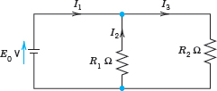
EXAMPLE 2 Gauss Elimination. Electrical Network
Solve the linear system

Derivation from the circuit in Fig. 159 (Optional). This is the system for the unknown currents x1 = i1, x2 = i2, x3 = i3 in the electrical network in Fig. 159. To obtain it, we label the currents as shown, choosing directions arbitrarily; if a current will come out negative, this will simply mean that the current flows against the direction of our arrow. The current entering each battery will be the same as the current leaving it. The equations for the currents result from Kirchhoff's laws:
Kirchhoff's Current Law (KCL).At any point of a circuit, the sum of the inflowing currents equals the sum of the outflowing currents.
Kirchhoff's Voltage Law (KVL).In any closed loop, the sum of all voltage drops equals the impressed electromotive force.
Node P gives the first equation, node Q the second, the right loop the third, and the left loop the fourth, as indicated in the figure.
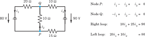
Fig. 159. Network in Example 2 and equations relating the currents
Solution by Gauss Elimination. This system could be solved rather quickly by noticing its particular form. But this is not the point. The point is that the Gauss elimination is systematic and will work in general, also for large systems. We apply it to our system and then do back substitution. As indicated, let us write the augmented matrix of the system first and then the system itself:

Step 1. Elimination of x1
Call the first row of A the pivot row and the first equation the pivot equation. Call the coefficient 1 of its x1-term the pivot in this step. Use this equation to eliminate x1 (get rid of x1) in the other equations. For this, do:
Add 1 times the pivot equation to the second equation.
Add −20 times the pivot equation to the fourth equation.
This corresponds to row operations on the augmented matrix as indicated in BLUE behind the new matrix in (3). So the operations are performed on the preceding matrix. The result is
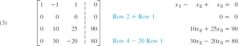
Step 2. Elimination of x2
The first equation remains as it is. We want the new second equation to serve as the next pivot equation. But since it has no x2-term (in fact, it is 0 = 0), we must first change the order of the equations and the corresponding rows of the new matrix. We put 0 = 0 at the end and move the third equation and the fourth equation one place up. This is called partial pivoting (as opposed to the rarely used total pivoting, in which the order of the unknowns is also changed). It gives

To eliminate x2, do:
Add −3 times the pivot equation to the third equation.
The result is
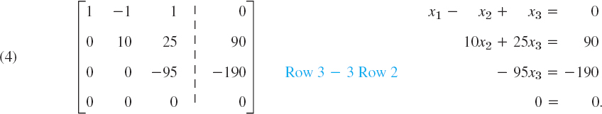
Back Substitution. Determination of x3, x2, x1 (in this order)
Working backward from the last to the first equation of this “triangular” system (4), we can now readily find x3, then x2, and then x1:
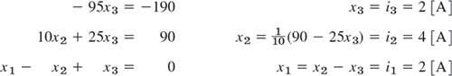
where A stands for “amperes.” This is the answer to our problem. The solution is unique.
Elementary Row Operations. Row-Equivalent Systems
Example 2 illustrates the operations of the Gauss elimination. These are the first two of three operations, which are called
Elementary Row Operations for Matrices:
Interchange of two rows
Addition of a constant multiple of one row to another row
Multiplication of a row by a nonzero constant c
CAUTION! These operations are for rows, not for columns! They correspond to the following
Elementary Operations for Equations:
Interchange of two equations
Addition of a constant multiple of one equation to another equation
Multiplication of an equation by a nonzero constant c
Clearly, the interchange of two equations does not alter the solution set. Neither does their addition because we can undo it by a corresponding subtraction. Similarly for their multiplication, which we can undo by multiplying the new equation by 1/c (since c ≠ 0), producing the original equation.
We now call a linear system S1 row-equivalent to a linear system S2 if S1 can be obtained from S2 by (finitely many!) row operations. This justifies Gauss elimination and establishes the following result.
Because of this theorem, systems having the same solution sets are often called equivalent systems. But note well that we are dealing with row operations. No column operations on the augmented matrix are permitted in this context because they would generally alter the solution set.
A linear system (1) is called overdetermined if it has more equations than unknowns, as in Example 2, determined if m = n, as in Example 1, and underdetermined if it has fewer equations than unknowns.
Furthermore, a system (1) is called consistent if it has at least one solution (thus, one solution or infinitely many solutions), but inconsistent if it has no solutions at all, as x1 + x2 = 1, x1 + x2 = 0 in Example 1, Case (c).
Gauss Elimination: The Three Possible Cases of Systems
We have seen, in Example 2, that Gauss elimination can solve linear systems that have a unique solution. This leaves us to apply Gauss elimination to a system with infinitely many solutions (in Example 3) and one with no solution (in Example 4).
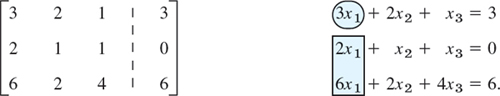
EXAMPLE 3 Gauss Elimination if Infinitely Many Solutions Exist
Solve the following linear system of three equations in four unknowns whose augmented matrix is
Solution. As in the previous example, we circle pivots and box terms of equations and corresponding entries to be eliminated. We indicate the operations in terms of equations and operate on both equations and matrices.
Step 1. Elimination of x1 from the second and third equations by adding

This gives the following, in which the pivot of the next step is circled.

Step 2. Elimination of x2 from the third equation of (6) by adding
![]()
This gives

Back Substitution. From the second equation, x2 = 1 − x3 + 4x4. From this and the first equation, x1 = 2 − x4. Since x3 and x4 remain arbitrary, we have infinitely many solutions. If we choose a value of x3 and a value of x4, then the corresponding values of x1 and x2 are uniquely determined.
On Notation. If unknowns remain arbitrary, it is also customary to denote them by other letters t1, t2, …. In this example we may thus write x1 = 2 − x4 = 2 − t2, x2 = 1 − x3 + 4x4 = 1 − t1 + 4t2, x3 = t1 (first arbitrary unknown), x4 = t2 (second arbitrary unknown).
EXAMPLE 4 Gauss Elimination if no Solution Exists
What will happen if we apply the Gauss elimination to a linear system that has no solution? The answer is that in this case the method will show this fact by producing a contradiction. For instance, consider
Step 1. Elimination of x1 from the second and third equations by adding


Step 2. Elimination of x2 from the third equation gives
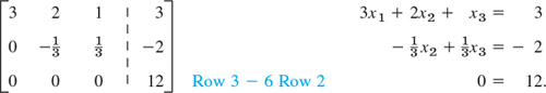
The false statement 0 = 12 shows that the system has no solution.
Row Echelon Form and Information From It
At the end of the Gauss elimination the form of the coefficient matrix, the augmented matrix, and the system itself are called the row echelon form. In it, rows of zeros, if present, are the last rows, and, in each nonzero row, the leftmost nonzero entry is farther to the right than in the previous row. For instance, in Example 4 the coefficient matrix and its augmented in row echelon form are

Note that we do not require that the leftmost nonzero entries be 1 since this would have no theoretic or numeric advantage. (The so-called reduced echelon form, in which those entries are 1, will be discussed in Sec. 7.8.)
The original system of m equations in n unknowns has augmented matrix [A|b]. This is to be row reduced to matrix [R|f]. The two systems Ax = b and Rx = f are equivalent: if either one has a solution, so does the other, and the solutions are identical.
At the end of the Gauss elimination (before the back substitution), the row echelon form of the augmented matrix will be

Here, r ![]() m, r11 ≠ 0, and all entries in the blue triangle and blue rectangle are zero.
m, r11 ≠ 0, and all entries in the blue triangle and blue rectangle are zero.
The number of nonzero rows, r, in the row-reduced coefficient matrix R is called the rank of R and also the rank of A. Here is the method for determining whether Ax = b has solutions and what they are:
- No solution. If r is less than m (meaning that R actually has at least one row of all 0s) and at least one of the numbers fr+1, fr+2, …, fm is not zero, then the system Rx = f is inconsistent: No solution is possible. Therefore the system Ax = b is inconsistent as well. See Example 4, where r = 2 < m = 3 and fr+1 = f3 = 12.
If the system is consistent (either r = m, or r < m and all the numbers fr+1, fr+2, …, fm are zero), then there are solutions.
- (b) Unique solution. If the system is consistent and r = n, there is exactly one solution, which can be found by back substitution. See Example 2, where r = n = 3 and m = 4.
- (c) Infinitely many solutions. To obtain any of these solutions, choose values of xr+1, …, xn arbitrarily. Then solve the rth equation for xr (in terms of those arbitrary values), then the (r − 1)st equation for xr−1, and so on up the line. See Example 3.
Orientation. Gauss elimination is reasonable in computing time and storage demand. We shall consider those aspects in Sec. 20.1 in the chapter on numeric linear algebra. Section 7.4 develops fundamental concepts of linear algebra such as linear independence and rank of a matrix. These in turn will be used in Sec. 7.5 to fully characterize the behavior of linear systems in terms of existence and uniqueness of solutions.
1–14 GAUSS ELIMINATION
Solve the linear system given explicitly or by its augmented matrix. Show details.
- 4x − 6y = −11
−3x + 8y = 10


- Equivalence relation. By definition, an equivalence relation on a set is a relation satisfying three conditions: (named as indicated)
- Each element A of the set is equivalent to itself (Reflexivity).
- If A is equivalent to B, then B is equivalent to A (Symmetry).
- If A is equivalent to B and B is equivalent to C, then A is equivalent to C (Transitivity).
Show that row equivalence of matrices satisfies these three conditions. Hint. Show that for each of the three elementary row operations these conditions hold.
- CAS PROJECT. Gauss Elimination and Back Substitution. Write a program for Gauss elimination and back substitution (a) that does not include pivoting and (b) that does include pivoting. Apply the programs to Probs. 11–14 and to some larger systems of your choice.
17–21 MODELS OF NETWORKS
In Probs. 17–19, using Kirchhoff's laws (see Example 2) and showing the details, find the currents:
- 17.

- 18.

- 19.
- 20. Wheatstone bridge. Show that if Rx/R3 = R1/R2 in the figure, then I = 0. (R0 is the resistance of the instrument by which I is measured.) This bridge is a method for determining Rx, R1, R2, R3 are known. R3 is variable. To get Rx, make I = 0 by varying R3. Then calculate Rx = R3R1/R2.

- 21. Traffic flow. Methods of electrical circuit analysis have applications to other fields. For instance, applying the analog of Kirchhoff's Current Law, find the traffic flow (cars per hour) in the net of one-way streets (in the directions indicated by the arrows) shown in the figure. Is the solution unique?
- 22. Models of markets. Determine the equilibrium solution (D1 = S1, D2 = S2) of the two-commodity market with linear model (D, S, P = demand, supply, price; index 1 = first commodity, index 2 = second commodity)
- 23. Balancing a chemical equation x1C3H8 + x2O2 → x3CO2 + x4H2O means finding integer x1, x2, x3, x4 such that the numbers of atoms of carbon (C), hydrogen (H), and oxygen (O) are the same on both sides of this reaction, in which propane C3H8 and O2 give carbon dioxide and water. Find the smallest positive integers x1, …, x4.
- 24. PROJECT. Elementary Matrices. The idea is that elementary operations can be accomplished by matrix multiplication. If A is an m × n matrix on which we want to do an elementary operation, then there is a matrix E such that EA is the new matrix after the operation. Such an E is called an elementary matrix. This idea can be helpful, for instance, in the design of algorithms. (Computationally, it is generally preferable to do row operations directly, rather than by multiplication by E.)
(a) Show that the following are elementary matrices, for interchanging Rows 2 and 3, for adding −5 times the first row to the third, and for multiplying the fourth row by 8.

Apply E1, E2, E3 to a vector and to a 4 × 3 matrix of your choice. Find B = E3E2E1A, where A = [ajk] is the general 4 × 2 matrix. Is B equal to C = E1E2E3A?
(b) Conclude that E1, E2, E3 are obtained by doing the corresponding elementary operations on the 4 × 4 unit matrix. Prove that if M is obtained from A by an elementary row operation, then

where E is obtained from the n × n unit matrix In by the same row operation.
7.4 Linear Independence. Rank of a Matrix. Vector Space
Since our next goal is to fully characterize the behavior of linear systems in terms of existence and uniqueness of solutions (Sec. 7.5), we have to introduce new fundamental linear algebraic concepts that will aid us in doing so. Foremost among these are linear independence and the rank of a matrix. Keep in mind that these concepts are intimately linked with the important Gauss elimination method and how it works.
Linear Independence and Dependence of Vectors
Given any set of m vectors a(1), …, a(m) (with the same number of components), a linear combination of these vectors is an expression of the form

where c1, c2, …, cm are any scalars. Now consider the equation

Clearly, this vector equation (1) holds if we choose all cj's zero, because then it becomes 0 = 0. If this is the only m-tuple of scalars for which (1) holds, then our vectors a(1), …, a(m) are said to form a linearly independent set or, more briefly, we call them linearly independent. Otherwise, if (1) also holds with scalars not all zero, we call these vectors linearly dependent. This means that we can express at least one of the vectors as a linear combination of the other vectors. For instance, if (1) holds with, say, c1 ≠ 0, we can solve (1) for a(1):
![]()
(Some kj's may be zero. Or even all of them, namely, if a(1) = 0.)
Why is linear independence important? Well, if a set of vectors is linearly dependent, then we can get rid of at least one or perhaps more of the vectors until we get a linearly independent set. This set is then the smallest “truly essential” set with which we can work. Thus, we cannot express any of the vectors, of this set, linearly in terms of the others.
EXAMPLE 1 Linear Independence and Dependence
The three vectors

are linearly dependent because
![]()
Although this is easily checked by vector arithmetic (do it!), it is not so easy to discover. However, a systematic method for finding out about linear independence and dependence follows below.
The first two of the three vectors are linearly independent because c1a(1) + c2a(2) = 0 implies c2 = 0 (from the second components) and then c1 = 0 (from any other component of a(1).
Rank of a Matrix
DEFINITION
The rank of a matrix A is the maximum number of linearly independent row vectors of A. It is denoted by rank A.
Our further discussion will show that the rank of a matrix is an important key concept for understanding general properties of matrices and linear systems of equations.
The matrix

has rank 2, because Example 1 shows that the first two row vectors are linearly independent, whereas all three row vectors are linearly dependent.
Note further that rank A = 0 if and only if A = 0. This follows directly from the definition.
We call a matrix A1 row-equivalent to a matrix A2 if A1 can be obtained from A2 by (finitely many!) elementary row operations.
Now the maximum number of linearly independent row vectors of a matrix does not change if we change the order of rows or multiply a row by a nonzero c or take a linear combination by adding a multiple of a row to another row. This shows that rank is invariant under elementary row operations:
Hence we can determine the rank of a matrix by reducing the matrix to row-echelon form, as was done in Sec. 7.3. Once the matrix is in row-echelon form, we count the number of nonzero rows, which is precisely the rank of the matrix.
EXAMPLE 3 Determination of Rank
For the matrix in Example 2 we obtain successively
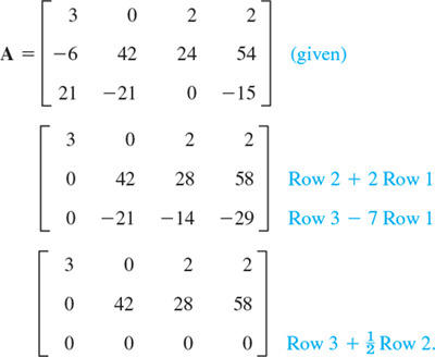
The last matrix is in row-echelon form and has two nonzero rows. Hence rank A = 2, as before.
Examples 1–3 illustrate the following useful theorem (with p = 3, n = 3, and the rank of the matrix = 2).
THEOREM 2 Linear Independence and Dependence of Vectors
Consider p vectors that each have n components. Then these vectors are linearly independent if the matrix formed, with these vectors as row vectors, has rank p. However, these vectors are linearly dependent if that matrix has rank less than p.
Further important properties will result from the basic
THEOREM 3 Rank in Terms of Column Vectors
The rank r of a matrix A equals the maximum number of linearly independent column vectors of A.
Hence A and its transpose AT have the same rank.
PROOF
In this proof we write simply “rows” and “columns” for row and column vectors. Let A be an m × n matrix of rank A = r. Then by definition of rank, A has r linearly independent rows which we denote by v(1), …, v(r) (regardless of their position in A), and all the rows a(1), …, a(m) of A are linear combinations of those, say,

These are vector equations for rows. To switch to columns, we write (3) in terms of components as n such systems, with k = 1, …, n,

and collect components in columns. Indeed, we can write (4) as
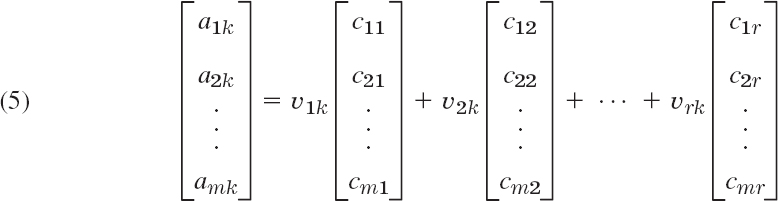
where k = 1, …, n. Now the vector on the left is the kth column vector of A. We see that each of these n columns is a linear combination of the same r columns on the right. Hence A cannot have more linearly independent columns than rows, whose number is rank A = r. Now rows of A are columns of the transpose AT. For AT our conclusion is that AT cannot have more linearly independent columns than rows, so that A cannot have more linearly independent rows than columns. Together, the number of linearly independent columns of A must be r, the rank of A. This completes the proof.
EXAMPLE 4 Illustration of Theorem 3
The matrix in (2) has rank 2. From Example 3 we see that the first two row vectors are linearly independent and by “working backward” we can verify that Row 3 = 6 Row ![]() Row 2. Similarly, the first two columns are linearly independent, and by reducing the last matrix in Example 3 by columns we find that
Row 2. Similarly, the first two columns are linearly independent, and by reducing the last matrix in Example 3 by columns we find that
![]()
Combining Theorems 2 and 3 we obtain
THEOREM 4 Linear Dependence of Vectors
Consider p vectors each having n components. If n < p, then these vectors are linearly dependent.
PROOF
The matrix A with those p vectors as row vectors has p rows and n < p columns; hence by Theorem 3 it has rank A ![]() n < p, which implies linear dependence by Theorem 2.
n < p, which implies linear dependence by Theorem 2.
Vector Space
The following related concepts are of general interest in linear algebra. In the present context they provide a clarification of essential properties of matrices and their role in connection with linear systems.
Consider a nonempty set V of vectors where each vector has the same number of components. If, for any two vectors a and b in V, we have that all their linear combinations αa + βb (α, β any real numbers) are also elements of V, and if, furthermore, a and b satisfy the laws (3a), (3c), (3d), and (4) in Sec. 7.1, as well as any vectors a, b, c in V satisfy (3b) then V is a vector space. Note that here we wrote laws (3) and (4) of Sec. 7.1 in lowercase letters a, b, c, which is our notation for vectors. More on vector spaces in Sec. 7.9.
The maximum number of linearly independent vectors in V is called the dimension of V and is denoted by dim V. Here we assume the dimension to be finite; infinite dimension will be defined in Sec. 7.9.
A linearly independent set in V consisting of a maximum possible number of vectors in V is called a basis for V. In other words, any largest possible set of independent vectors in V forms basis for V. That means, if we add one or more vector to that set, the set will be linearly dependent. (See also the beginning of Sec. 7.4 on linear independence and dependence of vectors.) Thus, the number of vectors of a basis for V equals dim V.
The set of all linear combinations of given vectors a(1), …, a(p) with the same number of components is called the span of these vectors. Obviously, a span is a vector space. If in addition, the given vectors a(1), …, a(p) are linearly independent, then they form a basis for that vector space.
This then leads to another equivalent definition of basis. A set of vectors is a basis for a vector space V if (1) the vectors in the set are linearly independent, and if (2) any vector in V can be expressed as a linear combination of the vectors in the set. If (2) holds, we also say that the set of vectors spans the vector space V.
By a subspace of a vector space V we mean a nonempty subset of V (including V itself) that forms a vector space with respect to the two algebraic operations (addition and scalar multiplication) defined for the vectors of V.
EXAMPLE 5 Vector Space, Dimension, Basis
The span of the three vectors in Example 1 is a vector space of dimension 2. A basis of this vector space consists of any two of those three vectors, for instance, a(1), a(2), or a(1), a(3), etc.
We further note the simple
The vector space Rn consisting of all vectors with n components (n real numbers) has dimension n.
PROOF
A basis of n vectors is a(1) = [1 0 … 0], a(2) = [0 1 0 … 0], …, a(n) = [0 … 0 1].
For a matrix A, we call the span of the row vectors the row space of A. Similarly, the span of the column vectors of A is called the column space of A.
Now, Theorem 3 shows that a matrix A has as many linearly independent rows as columns. By the definition of dimension, their number is the dimension of the row space or the column space of A. This proves
THEOREM 6 Row Space and Column Space
The row space and the column space of a matrix A have the same dimension, equal to rank A.
Finally, for a given matrix A the solution set of the homogeneous system Ax = 0 is a vector space, called the null space of A, and its dimension is called the nullity of A. In the next section we motivate and prove the basic relation

1–10 RANK, ROW SPACE, COLUMN SPACE
Find the rank. Find a basis for the row space. Find a basis for the column space. Hint. Row-reduce the matrix and its transpose. (You may omit obvious factors from the vectors of these bases.)


- CAS Experiment. Rank. (a) Show experimentally that the n × n matrix A = [ajk] with ajk = j + k − 1 has rank 2 for any n. (Problem 20 shows n = 4.) Try to prove it.
(b) Do the same when ajk = j + k + c, where c is any positive integer.
(c) What is rank A if ajk = 2j+k−2? Try to find other large matrices of low rank independent of n.
12–16 GENERAL PROPERTIES OF RANK
Show the following:
- 12. rank BTAT = rank AB. (Note the order!)
- 13. rank A = rank B does not imply rank A2 = rank B2. (Give a counterexample.)
- 14. If A is not square, either the row vectors or the column vectors of A are linearly dependent.
- 15. If the row vectors of a square matrix are linearly independent, so are the column vectors, and conversely.
- 16. Give examples showing that the rank of a product of matrices cannot exceed the rank of either factor.
17–25 LINEAR INDEPENDENCE
Are the following sets of vectors linearly independent? Show the details of your work.
- 17. [3 4 0 2], [2 −1 3 7], [1 16 −12 −22]
- 18.

- 19. [0 1 1]. [1 1 1], [0 0 1]
- 20. [1 2 3 4], [2 3 4 5], [3 4 5 6], [4 5 6 7]
- 21. [2 0 0 7], [2 0 0 8], [2 0 0 9], [2 0 1 0]
- 22. [0.4 −0.2 0.2], [0 0 0], [3.0 −0.6 1.5]
- 23. [9 8 7 6 5], [9 7 5 3 1]
- 24. [4 −1 3], [0 8 1], [1 3 −5], [2 6 1]
- 25. [6 0 −1 3], [2 2 5 0] [−4 −4 −4 −4]
- 26. Linearly independent subset. Beginning with the last of the vectors [3 0 1 2], [6 1 0 0], [12 1 2 4], [6 0 2 4], and [9 0 1 2] omit one after another until you get a linearly independent set.
Is the given set of vectors a vector space? Give reasons. If your answer is yes, determine the dimension and find a basis. (υ1, υ2, … denote components.)
- 27. All vectors in R3 with υ1 − υ2 + 2υ3 = 0
- 28. All vectors in R3 with 3υ2 + υ3 = k
- 29. All vectors in R2 with υ1
 υ2
υ2 - 30. All vectors in Rn with the first n − 2 components zero
- 31. All vectors in R5 with positive components
- 32. All vectors in R3 with 3υ1 − 2υ2 + υ3 = 0, 4υ1 + 5υ2 = 0
- 33. All vectors in R3 with 3υ1 − υ3 = 0, 2υ1 + 3υ2 − 4υ3 = 0
- 34. All vectors in Rn with |υj| = 1 for j = 1, …, n
- 35. All vectors in R4 with υ1 = 2υ2 = 3ν3 = 4υ4
7.5 Solutions of Linear Systems: Existence, Uniqueness
Rank, as just defined, gives complete information about existence, uniqueness, and general structure of the solution set of linear systems as follows.
A linear system of equations in n unknowns has a unique solution if the coefficient matrix and the augmented matrix have the same rank n, and infinitely many solutions if that common rank is less than n. The system has no solution if those two matrices have different rank.
To state this precisely and prove it, we shall use the generally important concept of a submatrix of A. By this we mean any matrix obtained from A by omitting some rows or columns (or both). By definition this includes A itself (as the matrix obtained by omitting no rows or columns); this is practical.
THEOREM 1 Fundamental Theorem for Linear Systems
(a) Existence. A linear system of m equations in n unknowns x1, …, xn

is consistent, that is, has solutions, if and only if the coefficient matrix A and the augmented matrix à have the same rank. Here,
(b) Uniqueness. The system (1) has precisely one solution if and only if this common rank r of A and à equals n.
(c) Infinitely many solutions.If this common rank r is less than n, the system (1) has infinitely many solutions. All of these solutions are obtained by determining r suitable unknowns (whose submatrix of coefficients must have rank r) in terms of the remaining n − r unknowns, to which arbitrary values can be assigned. (See Example 3 in Sec. 7.3.)
(d) Gauss elimination (Sec. 7.3).If solutions exist, they can all be obtained by the Gauss elimination. (This method will automatically reveal whether or not solutions exist; see Sec. 7.3.)
PROOF
(a) We can write the system (1) in vector form Ax = b or in terms of column vectors c(1), …, c(n) of A:
![]()
à is obtained by augmenting A by a single column b. Hence, by Theorem 3 in Sec. 7.4, rank à equals rank A or rank A + 1. Now if (1) has a solution x, then (2) shows that b must be a linear combination of those column vectors, so that à and A have the same maximum number of linearly independent column vectors and thus the same rank.
Conversely, if rank à = rank A, then b must be a linear combination of the column vectors of A, say,
![]()
since otherwise rank à = rank A + 1. But (2*) means that (1) has a solution, namely, x1 = α1, …, xn = αn, as can be seen by comparing (2*) and (2).
(b) If rank A = n, the n column vectors in (2) are linearly independent by Theorem 3 in Sec. 7.4. We claim that then the representation (2) of b is unique because otherwise
![]()
This would imply (take all terms to the left, with a minus sign)
![]()
and ![]() by linear independence. But this means that the scalars x1, …, xn in (2) are uniquely determined, that is, the solution of (1) is unique.
by linear independence. But this means that the scalars x1, …, xn in (2) are uniquely determined, that is, the solution of (1) is unique.
(c) If rank A = rank à = r < n, then by Theorem 3 in Sec. 7.4 there is a linearly independent set K of r column vectors of A such that the other n − r column vectors of A are linear combinations of those vectors. We renumber the columns and unknowns, denoting the renumbered quantities by ˆ, so that {ĉ(1), …, ĉ(r)} is that linearly independent set K. Then (2) becomes
![]()
![]() are linear combinations of the vectors of K, and so are the vectors
are linear combinations of the vectors of K, and so are the vectors ![]() . Expressing these vectors in terms of the vectors of K and collecting terms, we can thus write the system in the form
. Expressing these vectors in terms of the vectors of K and collecting terms, we can thus write the system in the form
![]()
with ![]() , where βj results from the n − r terms
, where βj results from the n − r terms ![]() ; here, j = 1, …, r. Since the system has a solution, there are y1, …, yr satisfying (3). These scalars are unique since K is linearly independent. Choosing
; here, j = 1, …, r. Since the system has a solution, there are y1, …, yr satisfying (3). These scalars are unique since K is linearly independent. Choosing ![]() fixes the βj and corresponding
fixes the βj and corresponding ![]() , where j = 1, …, r.
, where j = 1, …, r.
(d) This was discussed in Sec. 7.3 and is restated here as a reminder.
The theorem is illustrated in Sec. 7.3. In Example 2 there is a unique solution since rank à = rank A = n = 3 (as can be seen from the last matrix in the example). In Example 3 we have rank à = rank A = 2 < n = 4 and can choose x3 and x4 arbitrarily. In Example 4 there is no solution because rank A = 2 < rank à = 3.
Homogeneous Linear System
Recall from Sec. 7.3 that a linear system (1) is called homogeneous if all the bj's are zero, and nonhomogeneous if one or several bj's are not zero. For the homogeneous system we obtain from the Fundamental Theorem the following results.
THEOREM 2 Homogeneous Linear System
A homogeneous linear system
always has the trivial solution x1 = 0, …, xn = 0. Nontrivial solutions exist if and only if rank A < n. If rank A = r < n, these solutions, together with x = 0, form a vector space (see Sec. 7.4) of dimension n − r called the solution space of (4).
In particular, if x(1) and x(2) are solution vectors of (4), then x = c1x(1) + c2x(2) with any scalars c1 and c2 is a solution vector of (4). (This does not hold for nonhomogeneous systems. Also, the term solution space is used for homogeneous systems only.)
PROOF
The first proposition can be seen directly from the system. It agrees with the fact that b = 0 implies that rank à = rank A, so that a homogeneous system is always consistent. If rank A = n, the trivial solution is the unique solution according to (b) in Theorem 1. If rank A < n, there are nontrivial solutions according to (c) in Theorem 1. The solutions form a vector space because if x(1) and x(2) are any of them, then Ax(1) = 0, Ax(2) = 0, and this implies A(x(1) + x(2)) = Ax(1) + Ax(2) = 0 as well as A(cx(1)) = cAx(1) = 0, where c is arbitrary. If rank A = r < n, Theorem 1 (c) implies that we can choose n − r suitable unknowns, call them xr+1, …, xn, in an arbitrary fashion, and every solution is obtained in this way. Hence a basis for the solution space, briefly called a basis of solutions of (4), is y(1), …, y(n−r), where the basis vector y(j) is obtained by choosing xr+j = 1 and the other xr+1, …, xn zero; the corresponding first r components of this solution vector are then determined. Thus the solution space of (4) has dimension n − r. This proves Theorem 2.
The solution space of (4) is also called the null space of A because Ax = 0 for every x in the solution space of (4). Its dimension is called the nullity of A. Hence Theorem 2 states that

where n is the number of unknowns (number of columns of A).
Furthermore, by the definition of rank we have rank A ![]() m in (4). Hence if m < n, then rank A < n. By Theorem 2 this gives the practically important
m in (4). Hence if m < n, then rank A < n. By Theorem 2 this gives the practically important
THEOREM 3 Homogeneous Linear System with Fewer Equations Than Unknowns
A homogeneous linear system with fewer equations than unknowns always has nontrivial solutions.
Nonhomogeneous Linear Systems
The characterization of all solutions of the linear system (1) is now quite simple, as follows.
THEOREM 4 Nonhomogeneous Linear System
If a nonhomogeneous linear system (1) is consistent, then all of its solutions are obtained as
![]()
where x0 is any (fixed) solution of (1) and xh runs through all the solutions of the corresponding homogeneous system (4).
PROOF
The difference xh = x − x0 of any two solutions of (1) is a solution of (4) because Axh = A(x − x0) = Ax − Ax0 = b − b = 0. Since x is any solution of (1), we get all the solutions of (1) if in (6) we take any solution x0 of (1) and let xh vary throughout the solution space of (4).
This covers a main part of our discussion of characterizing the solutions of systems of linear equations. Our next main topic is determinants and their role in linear equations.
7.6 For Reference: Second- and Third-Order Determinants
We created this section as a quick general reference section on second- and third-order determinants. It is completely independent of the theory in Sec. 7.7 and suffices as a reference for many of our examples and problems. Since this section is for reference, go on to the next section, consulting this material only when needed.
A determinant of second order is denoted and defined by
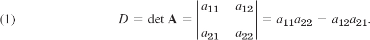
So here we have bars (whereas a matrix has brackets).
Cramer's rule for solving linear systems of two equations in two unknowns

is

with D as in (1), provided
![]()
The value D = 0 appears for homogeneous systems with nontrivial solutions.
PROOF
We prove (3). To eliminate x2 multiply (2a) by a22 and (2b) by −a12 and add,
![]()
Similarly, to eliminate x1 multiply (2a) by −a21 and (2b) by a11 and add,
![]()
Assuming that D = a11a22 − a12a21 ≠ 0, dividing, and writing the right sides of these two equations as determinants, we obtain (3).

Third-Order Determinants
A determinant of third order can be defined by
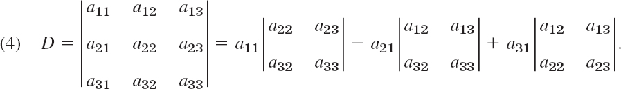
Note the following. The signs on the right are + − +. Each of the three terms on the right is an entry in the first column of D times its minor, that is, the second-order determinant obtained from D by deleting the row and column of that entry; thus, for a11 delete the first row and first column, and so on.
If we write out the minors in (4), we obtain
![]()
Cramer's Rule for Linear Systems of Three Equations

is

with the determinant D of the system given by (4) and

Note that D1, D2, D3 are obtained by replacing Columns 1, 2, 3, respectively, by the column of the right sides of (5).
Cramer's rule (6) can be derived by eliminations similar to those for (3), but it also follows from the general case (Theorem 4) in the next section.
7.7 Determinants. Cramer's Rule
Determinants were originally introduced for solving linear systems. Although impractical in computations, they have important engineering applications in eigenvalue problems (Sec. 8.1), differential equations, vector algebra (Sec. 9.3), and in other areas. They can be introduced in several equivalent ways. Our definition is particularly for dealing with linear systems.
A determinant of ordern is a scalar associated with an n × n (hence square !) matrix A = [ajk], and is denoted by
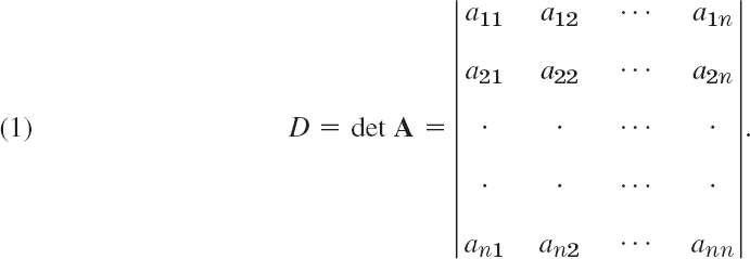
For n = 1, this determinant is defined by
![]()
For n ![]() 2 by
2 by
![]()
or
![]()
Here,
![]()
and Mjk is a determinant of order n − 1 namely, the determinant of the submatrix of A obtained from A by omitting the row and column of the entry ajk, that is, the jth row and the kth column.
In this way, D is defined in terms of n determinants of order n − 1, each of which is, in turn, defined in terms of n − 1 determinants of order n − 2, and so on—until we finally arrive at second-order determinants, in which those submatrices consist of single entries whose determinant is defined to be the entry itself.
From the definition it follows that we mayexpand D by any row or column, that is, choose in (3) the entries in any row or column, similarly when expanding the Cjk's in (3), and so on.
This definition is unambiguous, that is, it yields the same value for D no matter which columns or rows we choose in expanding. A proof is given in App. 4.
Terms used in connection with determinants are taken from matrices. In D we have n2 entries ajk, also n rows and n columns, and a main diagonal on which a11, a22, …, ann stand. Two terms are new:
Mjk is called the minor of ajk in D, and Cjk the cofactor of ajk in D.
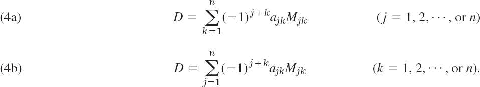
For later use we note that (3) may also be written in terms of minors
EXAMPLE 1 Minors and Cofactors of a Third-Order Determinant
In (4) of the previous section the minors and cofactors of the entries in the first column can be seen directly. For the entries in the second row the minors are

and the cofactors are C21 = −M21, C22 = +M22, and C23 = −M23. Similarly for the third row—write these down yourself. And verify that the signs in Cjk form a checkerboard pattern

EXAMPLE 2 Expansions of a Third-Order Determinant
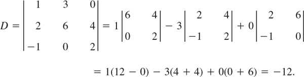
This is the expansion by the first row. The expansion by the third column is
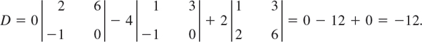
Verify that the other four expansions also give the value −12.
EXAMPLE 3 Determinant of a Triangular Matrix

Inspired by this, can you formulate a little theorem on determinants of triangular matrices? Of diagonal matrices?
General Properties of Determinants
There is an attractive way of finding determinants (1) that consists of applying elementary row operations to (1). By doing so we obtain an “upper triangular” determinant (see Sec. 7.1, for definition with “matrix” replaced by “determinant”) whose value is then very easy to compute, being just the product of its diagonal entries. This approach is similar (but not the same !) to what we did to matrices in Sec. 7.3. In particular, be aware that interchanging two rows in a determinant introduces a multiplicative factor of −1 to the value of the determinant! Details are as follows.
THEOREM 1 Behavior of an nth-Order Determinant under Elementary Row Operations
(a) Interchange of two rows multiplies the value of the determinant by −1.
(b) Addition of a multiple of a row to another row does not alter the value of the determinant.
(c) Multiplication of a row by a nonzero constant c multiplies the value of the determinant by c. (This holds also when c = 0, but no longer gives an elementary row operation.)
PROOF
(a) By induction. The statement holds for n = 2 because

We now make the induction hypothesis that (a) holds for determinants of order n − 1 ![]() 2 and show that it then holds for determinants of order n. Let D be of order n. Let E be obtained from D by the interchange of two rows. Expand D and E by a row that is not one of those interchanged, call it the jth row. Then by (4a),
2 and show that it then holds for determinants of order n. Let D be of order n. Let E be obtained from D by the interchange of two rows. Expand D and E by a row that is not one of those interchanged, call it the jth row. Then by (4a),

where Njk is obtained from the minor Mjk of ajk in D by the interchange of those two rows which have been interchanged in D (and which Njk must both contain because we expand by another row!). Now these minors are of order n − 1. Hence the induction hypothesis applies and gives Njk = −Mjk. Thus E = −D by (5).
(b) Add c times Row i to Row j. Let ![]() be the new determinant. Its entries in Row j are ajk + caik. If we expand
be the new determinant. Its entries in Row j are ajk + caik. If we expand ![]() by this Row j, we see that we can write it as
by this Row j, we see that we can write it as ![]() , where D1 = D has in Row j the ajk, whereas D2 has in that Row j the ajk from the addition. Hence D2 has ajk in both Row i and Row j. Interchanging these two rows gives D2 back, but on the other hand it gives −D2 by (a). Together D2 = −D2 = 0, so that
, where D1 = D has in Row j the ajk, whereas D2 has in that Row j the ajk from the addition. Hence D2 has ajk in both Row i and Row j. Interchanging these two rows gives D2 back, but on the other hand it gives −D2 by (a). Together D2 = −D2 = 0, so that ![]() .
.
(c) Expand the determinant by the row that has been multiplied.
CAUTION! det (cA) cn det A (not c det A). Explain why.
EXAMPLE 4 Evaluation of Determinants by Reduction to Triangular Form
Because of Theorem 1 we may evaluate determinants by reduction to triangular form, as in the Gauss elimination for a matrix. For instance (with the blue explanations always referring to the preceding determinant)

THEOREM 2 Further Properties of nth-Order Determinants
(a)–(c) in Theorem 1 hold also for columns.
(d) Transposition leaves the value of a determinant unaltered.
(e) A zero row or column renders the value of a determinant zero.
(f) Proportional rows or columns render the value of a determinant zero. In particular, a determinant with two identical rows or columns has the value zero.
PROOF
(a)–(e) follow directly from the fact that a determinant can be expanded by any row column. In (d), transposition is defined as for matrices, that is, the jth row becomes the jth column of the transpose.
(f) If Row j = c times Row i, then D = cD1, where D1 has Row j = Row i. Hence an interchange of these rows reproduces D1, but it also gives −D1 by Theorem 1(a). Hence D1 = 0 and D = cD1 = 0. Similarly for columns.
It is quite remarkable that the important concept of the rank of a matrix A, which is the maximum number of linearly independent row or column vectors of A (see Sec. 7.4), can be related to determinants. Here we may assume that rank A > 0 because the only matrices with rank 0 are the zero matrices (see Sec. 7.4).
THEOREM 3 Rank in Terms of Determinants
Consider an m × n matrix A = [ajk]:
- A has rank r 1 if and only if A has an r × r submatrix with a nonzero determinant.
- The determinant of any square submatrix with more than r rows, contained in A (if such a matrix exists!) has a value equal to zero.
Furthermore, if m = n, we have:
- (3) An n × n square matrix A has rank n if and only if
![]()
PROOF
The key idea is that elementary row operations (Sec. 7.3) alter neither rank (by Theorem 1 in Sec. 7.4) nor the property of a determinant being nonzero (by Theorem 1 in this section). The echelon form  of A (see Sec. 7.3) has r nonzero row vectors (which are the first r row vectors) if and only if rank A = r. Without loss of generality, we can assume that r ![]() 1. Let
1. Let ![]() be the r × r submatrix in the left upper corner of  (so that the entries of
be the r × r submatrix in the left upper corner of  (so that the entries of ![]() are in both the first r rows and r columns of Â). Now
are in both the first r rows and r columns of Â). Now ![]() is triangular, with all diagonal entries rjj nonzero. Thus, det
is triangular, with all diagonal entries rjj nonzero. Thus, det ![]() . Also det R ≠ 0 for the corresponding r × r submatrix R of A because
. Also det R ≠ 0 for the corresponding r × r submatrix R of A because ![]() results from R by elementary row operations. This proves part (1).
results from R by elementary row operations. This proves part (1).
Similarly, det S = 0 for any square submatrix S of r + 1 or more rows perhaps contained in A because the corresponding submatrix ![]() of  must contain a row of zeros (otherwise we would have rank A
of  must contain a row of zeros (otherwise we would have rank A ![]() r + 1), so that det
r + 1), so that det ![]() by Theorem 2. This proves part (2). Furthermore, we have proven the theorem for an m × n matrix.
by Theorem 2. This proves part (2). Furthermore, we have proven the theorem for an m × n matrix.
For an n × n square matrix A we proceed as follows. To prove (3), we apply part (1) (already proven!). This gives us that rank A = n ![]() 1 if and only if A contains an n × n submatrix with nonzero determinant. But the only such submatrix contained in our square matrix A, is A itself, hence det A ≠ 0. This proves part (3).
1 if and only if A contains an n × n submatrix with nonzero determinant. But the only such submatrix contained in our square matrix A, is A itself, hence det A ≠ 0. This proves part (3).
Cramer's Rule
Theorem 3 opens the way to the classical solution formula for linear systems known as Cramer's rule,2 which gives solutions as quotients of determinants. Cramer's rule is not practical in computations for which the methods in Secs. 7.3 and 20.1–20.3 are suitable. However, Cramer's rule is of theoretical interest in differential equations (Secs. 2.10 and 3.3) and in other theoretical work that has engineering applications.
THEOREM 4 Cramer's Theorem (Solution of Linear Systems by Determinants)
(a) If a linear system of n equations in the same number of unknowns x1, …, xn

has a nonzero coefficient determinant D = det A, the system has precisely one solution. This solution is given by the formulas
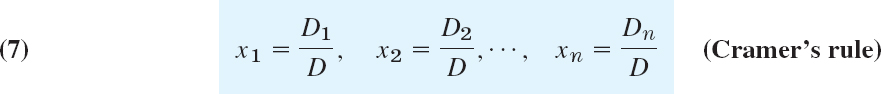
where Dk is the determinant obtained from D by replacing in D the kth column by the column with the entries b1, …, bn.
(b)Hence if the system (6) is homogeneous and D ≠ 0, it has only the trivial solution x1 = 0, x2 = 0, …, xn = 0. If D = 0, the homogeneous system also has nontrivial solutions.
PROOF
The augmented matrix ![]() of the system (6) is of size n × (n + 1). Hence its rank can be at most n. Now if
of the system (6) is of size n × (n + 1). Hence its rank can be at most n. Now if
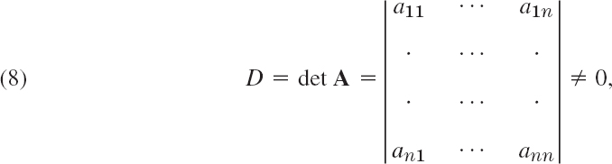
then rank A = n by Theorem 3. Thus rank à = rank A. Hence, by the Fundamental Theorem in Sec. 7.5, the system (6) has a unique solution.
Let us now prove (7). Expanding D by its kth column, we obtain
![]()
where Cik is the cofactor of entry aik in D. If we replace the entries in the kth column of D by any other numbers, we obtain a new determinant, say, ![]() . Clearly, its expansion by the kth column will be of the form (9), with a1k, …, ank replaced by those new numbers and the cofactors Cik as before. In particular, if we choose as new numbers the entries a1l, …, anl of the lth column of D (where l ≠ k), we have a new determinant
. Clearly, its expansion by the kth column will be of the form (9), with a1k, …, ank replaced by those new numbers and the cofactors Cik as before. In particular, if we choose as new numbers the entries a1l, …, anl of the lth column of D (where l ≠ k), we have a new determinant ![]() which has the column [a1l … anl]T twice, once as its lth column, and once as its kth because of the replacement. Hence
which has the column [a1l … anl]T twice, once as its lth column, and once as its kth because of the replacement. Hence ![]() by Theorem 2(f). If we now expand
by Theorem 2(f). If we now expand ![]() by the column that has been replaced (the kth column), we thus obtain
by the column that has been replaced (the kth column), we thus obtain
![]()
We now multiply the first equation in (6) by C1k on both sides, the second by C2k, …, the last by Cnk and add the resulting equations. This gives

Collecting terms with the same xj, we can write the left side as
![]()
From this we see that xk is multiplied by
![]()
Equation (9) shows that this equals D. Similarly, x1 is multiplied by
![]()
Equation (10) shows that this is zero when l ≠ k. Accordingly, the left side of (11) equals simply xkD so that (11) becomes
![]()
Now the right side of this is Dk as defined in the theorem, expanded by its kth column, so that division by D gives (7). This proves Cramer's rule.
If (6) is homogeneous and D ≠ 0, then each Dk has a column of zeros, so that Dk = 0 by Theorem 2(e), and (7) gives the trivial solution.
Finally, if (6) is homogeneous and D = 0, then rank A < n by Theorem 3, so that nontrivial solutions exist by Theorem 2 in Sec. 7.5.
EXAMPLE 5 Illustration of Cramer's Rule (Theorem 4)
For n = 2, see Example 1 of Sec. 7.6. Also, at the end of that section, we give Cramer's rule for a general linear system of three equations.
Finally, an important application for Cramer's rule dealing with inverse matrices will be given in the next section.
1–6 GENERAL PROBLEMS
- General Properties of Determinants. Illustrate each statement in Theorems 1 and 2 with an example of your choice.
- Second-Order Determinant. Expand a general second-order determinant in four possible ways and show that the results agree.
- Third-Order Determinant. Do the task indicated in Theorem 2. Also evaluate D by reduction to triangular form.
- Expansion Numerically Impractical. Show that the computation of an nth-order determinant by expansion involves n! multiplications, which if a multiplication takes 10−9 sec would take these times:

- Multiplication by Scalar. Show that det(kA) = kn det A (not k det A). Give an example.
- Minors, cofactors. Complete the list in Example 1.
7–15 EVALUATION OF DETERMINANTS
Showing the details, evaluate:
- 7.

- 8.

- 9.
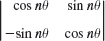
- 10.

- 11.

- 12.

- 13.
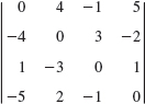
- 14.

- 15.
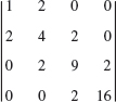
- 16. CAS EXPERIMENT. Determinant of Zeros and Ones. Find the value of the determinant of the n × n matrix An with main diagonal entries all 0 and all others 1. Try to find a formula for this. Try to prove it by induction. Interpret A3 and A4 as incidence matrices (as in Problem Set 7.1 but without the minuses) of a triangle and a tetrahedron, respectively; similarly for an n-simplex, having n vertices and n(n − 1)/2 edges (and spanning Rn−1, n = 5, 6, …).
17–19 RANK BY DETERMINANTS
Find the rank by Theorem 3 (which is not very practical) and check by row reduction. Show details.
- 17.

- 18.

- 19.

- 20. TEAM PROJECT. Geometric Applications: Curves and Surfaces Through Given Points. The idea is to get an equation from the vanishing of the determinant of a homogeneous linear system as the condition for a nontrivial solution in Cramer's theorem. We explain the trick for obtaining such a system for the case of a line L through two given points P1: (x1, y1) and P2: (x2, y2). The unknown line is ax + by = −c, say. We write it as ax + by + c · 1 = 0. To get a nontrivial solution a, b, c, the determinant of the “coefficients” x, y, 1 must be zero. The system is

(a) Line through two points. Derive from D = 0 in (12) the familiar formula
(b) Plane. Find the analog of (12) for a plane through three given points. Apply it when the points are (1, 1, 1), (3, 2, 6), (5, 0, 5).
(c) Circle. Find a similar formula for a circle in the plane through three given points. Find and sketch the circle through (2, 6), (6, 4), (7, 1).
(d) Sphere. Find the analog of the formula in (c) for a sphere through four given points. Find the sphere through (0, 0, 5), (4, 0, 1), (0, 4, 1), (0, 0, −3) by this formula or by inspection.
(e) General conic section. Find a formula for a general conic section (the vanishing of a determinant of 6th order). Try it out for a quadratic parabola and for a more general conic section of your own choice.
21–25 CRAMER'S RULE
Solve by Cramer's rule. Check by Gauss elimination and back substitution. Show details.
- 21.

- 22.

- 23.

- 24.
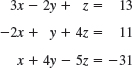
- 25.

7.8 Inverse of a Matrix. Gauss–Jordan Elimination
In this section we consider square matrices exclusively.
The inverse of an n × n matrix A = [ajk] is denoted by A−1 and is an n × n matrix such that
![]()
where I is the n × n unit matrix (see Sec. 7.2).
If A has an inverse, then A is called a nonsingular matrix. If A has no inverse, then A is called a singular matrix.
If A has an inverse, the inverse is unique.
Indeed, if both B and C are inverses of A, then AB = I and CA = I, so that we obtain the uniqueness from
![]()
We prove next that A has an inverse (is nonsingular) if and only if it has maximum possible rank n. The proof will also show that Ax = b implies x = A−1b provided A−1 exists, and will thus give a motivation for the inverse as well as a relation to linear systems. (But this will not give a good method of solving Ax = b numerically because the Gauss elimination in Sec. 7.3 requires fewer computations.)
THEOREM 1 Existence of the Inverse
The inverse A−1 of an n × n matrix A exists if and only if rank A = n, thus (by Theorem 3, Sec. 7.7) if and only if det A ≠ 0. Hence A is nonsingular if rank A = n, and is singular if. rank A < n.
Let A be a given n × n matrix and consider the linear system
![]()
If the inverse A−1 exists, then multiplication from the left on both sides and use of (1) gives
![]()
This shows that (2) has a solution x, which is unique because, for another solution u, we have Au = b, so that u = A−1b = x. Hence A must have rank n by the Fundamental Theorem in Sec. 7.5.
Conversely, let rank A = n. Then by the same theorem, the system (2) has a unique solution x for any b. Now the back substitution following the Gauss elimination (Sec. 7.3) shows that the components xj of x are linear combinations of those of b. Hence we can write
![]()
with B to be determined. Substitution into (2) gives
![]()
for any b. Hence C = AB = I, the unit matrix. Similarly, if we substitute (2) into (3) we get
![]()
for any x (and b = Ax). Hence BA = I. Together, B = A−1 exists.
Determination of the Inverse by the Gauss–Jordan Method
To actually determine the inverse A−1 of a nonsingular n × n matrix A, we can use a variant of the Gauss elimination (Sec. 7.3), called the Gauss–Jordan elimination.3 The idea of the method is as follows.
Using A, we form n linear systems
![]()
where the vectors e(1), …, e(n) are the columns of the n × n unit matrix I; thus, e(1) = [1 0 … 0]T, e(2) = [0 1 0 … 0]T, etc. These are n vector equations in the unknown vectors x(1), …, x(n). We combine them into a single matrix equation AX = I, with the unknown matrix X having the columns x(1), …, x(n). Correspondingly, we combine the n augmented matrices [A e(1)], …, [A e(n)] into one wide n × 2n “augmented matrix” ![]() . Now multiplication of AX = I by A−1 from the left gives X = A−1I = A−1. Hence, to solve AX = I for X, we can apply the Gauss elimination to
. Now multiplication of AX = I by A−1 from the left gives X = A−1I = A−1. Hence, to solve AX = I for X, we can apply the Gauss elimination to ![]() . This gives a matrix of the form [U H] with upper triangular U because the Gauss elimination triangularizes systems. The Gauss–Jordan method reduces U by further elementary row operations to diagonal form, in fact to the unit matrix I. This is done by eliminating the entries of U above the main diagonal and making the diagonal entries all 1 by multiplication (see Example 1). Of course, the method operates on the entire matrix [U H], transforming H into some matrix K, hence the entire [U H] to [I K]. This is the “augmented matrix” of IX = K. Now IX = X = A−1, as shown before. By comparison, K = A−1, so that we can read A−1 directly from [I K].
. This gives a matrix of the form [U H] with upper triangular U because the Gauss elimination triangularizes systems. The Gauss–Jordan method reduces U by further elementary row operations to diagonal form, in fact to the unit matrix I. This is done by eliminating the entries of U above the main diagonal and making the diagonal entries all 1 by multiplication (see Example 1). Of course, the method operates on the entire matrix [U H], transforming H into some matrix K, hence the entire [U H] to [I K]. This is the “augmented matrix” of IX = K. Now IX = X = A−1, as shown before. By comparison, K = A−1, so that we can read A−1 directly from [I K].
The following example illustrates the practical details of the method.
EXAMPLE 1 Finding the Inverse of a Matrix by Gauss–Jordan Elimination
Determine the inverse A−1 of
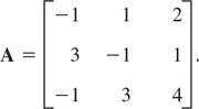
Solution. We apply the Gauss elimination (Sec. 7.3) to the following n × 2n = 3 × 6 matrix, where BLUE always refers to the previous matrix.
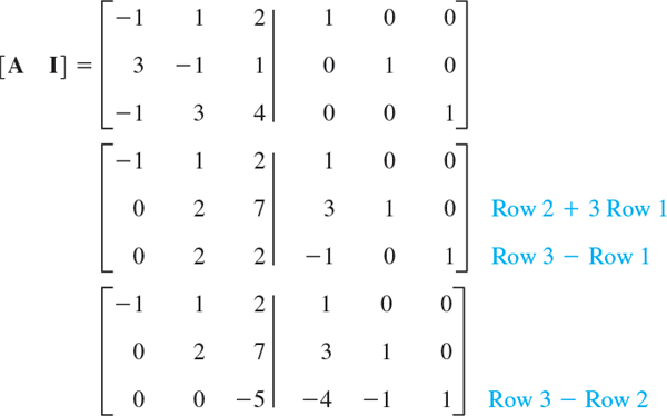
This is [U H] as produced by the Gauss elimination. Now follow the additional Gauss–Jordan steps, reducing U to I, that is, to diagonal form with entries 1 on the main diagonal.
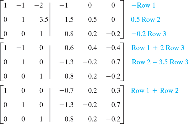
The last three columns constitute A−1. Check:
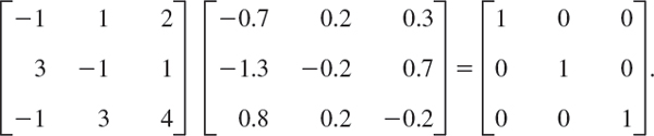
Hence AA−1 = I. Similarly, A−1A = I.
Formulas for Inverses
Since finding the inverse of a matrix is really a problem of solving a system of linear equations, it is not surprising that Cramer's rule (Theorem 4, Sec. 7.7) might come into play. And similarly, as Cramer's rule was useful for theoretical study but not for computation, so too is the explicit formula (4) in the following theorem useful for theoretical considerations but not recommended for actually determining inverse matrices, except for the frequently occurring 2 × 2 case as given in (4*).
THEOREM 2 Inverse of a Matrix by Determinants
The inverse of a nonsingular n × n matrix A = [ajk] is given by
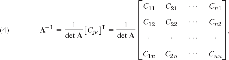
where Cjk is the cofactor of ajk in det A (see Sec. 7.7). (CAUTION! Note well that in A−1, the cofactor Cjk occupies the same place as akj (not ajk) does in A.)
In particular, the inverse of

PROOF
We denote the right side of (4) by B and show that BA = I. We first write
![]()
and then show that G = I. Now by the definition of matrix multiplication and because of the form of B in (4), we obtain (CAUTION! Csk not Cks)

Now (9) and (10) in Sec. 7.7 show that the sum (…) on the right is D = det A when l = k, and is zero when l ≠ k. Hence
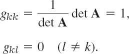
In particular, for n = 2 we have in (4), in the first row, C11 = a22, C21 = −a12 and, in the second row, C12 = −a21, C22 = a11. This gives (4*).
The special case n = 2 occurs quite frequently in geometric and other applications. You may perhaps want to memorize formula (4*). Example 2 gives an illustration of (4*).

EXAMPLE 3 Further Illustration of Theorem 2
Using (4), find the inverse of

Solution. We obtain A = −1(−7) − 1 · 13 + 2 · 8 = 10, and in (4),
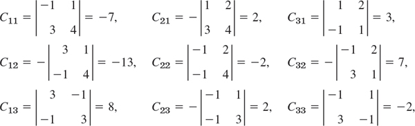
so that by (4), in agreement with Example 1,
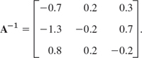
Diagonal matrices A = [ajk], ajk = 0 when j ≠ k, have an inverse if and only if all ajj ≠ 0. Then A−1 is diagonal, too, with entries 1/a11, …, 1/ann.
PROOF
For a diagonal matrix we have in (4)
![]()
EXAMPLE 4 Inverse of a Diagonal Matrix
Let

Then we obtain the inverse A−1 by inverting each individual diagonal element of A, that is, by taking ![]() , and
, and ![]() as the diagonal entries of A−1, that is,
as the diagonal entries of A−1, that is,

Products can be inverted by taking the inverse of each factor and multiplying these inverses in reverse order,

Hence for more than two factors,
![]()
PROOF
The idea is to start from (1) for AC instead of A, that is, AC(AC)−1 = I, and multiply it on both sides from the left, first by A−1, which because of A−1A = I gives
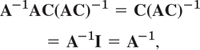
and then multiplying this on both sides from the left, this time by C−1 and by using C−1C = I.
![]()
This proves (7), and from it, (8) follows by induction.
We also note that the inverse of the inverse is the given matrix, as you may prove,
![]()
Unusual Properties of Matrix Multiplication. Cancellation Laws
Section 7.2 contains warnings that some properties of matrix multiplication deviate from those for numbers, and we are now able to explain the restricted validity of the so-called cancellation laws [2] and [3] below, using rank and inverse, concepts that were not yet available in Sec. 7.2. The deviations from the usual are of great practical importance and must be carefully observed. They are as follows.
[1] Matrix multiplication is not commutative, that is, in general we have
![]()
[2] AB = 0 does not generally imply A = 0 or B = 0 (or BA = 0); for example,
[3] AC = AD does not generally imply C = D (even when A ≠ 0).
Complete answers to [2] and [3] are contained in the following theorem.
Let A, B, C be n × n matrices. Then:
- If rank A = n and AB = AC, then B = C.
- Let rank A = n, then AB = 0 implies B = 0. Hence if, AB = 0, but A ≠ 0 as well as, B ≠ 0 then rank A < n and rank B < n.
- If A is singular, so are BA and AB.
PROOF
(a) The inverse of A exists by Theorem 1. Multiplication by A−1 from the left gives A−1AB = A−1AC, hence B = C.
(b) Let rank A = n. Then A−1 exists, and AB = 0 implies A−1AB = B = 0. Similarly when rank B = n. This implies the second statement in (b).
(c1) Rank A < n by Theorem 1. Hence Ax = 0 has nontrivial solutions by Theorem 2 in Sec. 7.5. Multiplication by B shows that these solutions are also solutions of BAx = 0, so that rank (BA) < n by Theorem 2 in Sec. 7.5 and BA is singular by Theorem 1.
(c2) AT is singular by Theorem 2(d) in Sec. 7.7. Hence BTAT is singular by part (c1), and is equal to (AB)T by (10d) in Sec. 7.2. Hence AB is singular by Theorem 2(d) in Sec. 7.7.
Determinants of Matrix Products
The determinant of a matrix product AB or BA can be written as the product of the determinants of the factors, and it is interesting that det AB = det BA, although AB ≠ BA in general. The corresponding formula (10) is needed occasionally and can be obtained by Gauss–Jordan elimination (see Example 1) and from the theorem just proved.

If A or B is singular, so are AB and BA by Theorem 3(c), and (10) reduces to 0 = 0 by Theorem 3 in Sec. 7.7.
Now let A and B be nonsingular. Then we can reduce A to a diagonal matrix  = [ajk] by Gauss–Jordan steps. Under these operations, det A retains its value, by Theorem 1 in Sec. 7.7, (a) and (b) [not (c)] except perhaps for a sign reversal in row interchanging when pivoting. But the same operations reduce AB to ÂB with the same effect on det(AB). Hence it remains to prove (10) for ÂB; written out,
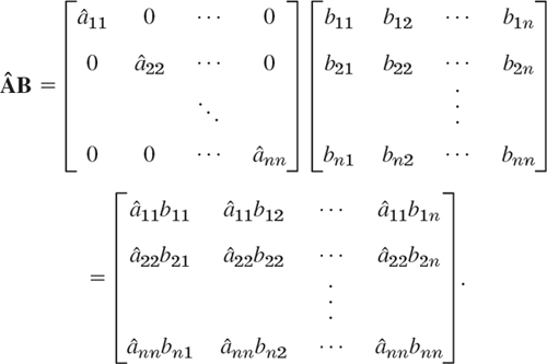
We now take the determinant (ÂB). On the right we can take out a factor â11 from the first row, â22 from the second, …, ânn from the nth. But this product â11â22 … ânn equals  because  is diagonal. The remaining determinant is det B. This proves (10) for det (AB), and the proof for det (BA) follows by the same idea.
This completes our discussion of linear systems (Secs. 7.3–7.8). Section 7.9 on vector spaces and linear transformations is optional. Numeric methods are discussed in Secs. 20.1–20.4, which are independent of other sections on numerics.
1–10 INVERSE
Find the inverse by Gauss–Jordan (or by (4*) if n = 2). Check by using (1).


11–18 SOME GENERAL FORMULAS
- 11. Inverse of the square. Verify (A2)−1 = (A−1)2 for A in Prob. 1.
- 12. Prove the formula in Prob. 11.
- 13. Inverse of the transpose. Verify (AT)−1 = (A−1)T for A in Prob. 1.
- 14. Prove the formula in Prob. 13.
- 15. Inverse of the inverse. Prove that (A−1)−1 = A.
- 16. Rotation. Give an application of the matrix in Prob. 2 that makes the form of the inverse obvious.
- 17. Triangular matrix. Is the inverse of a triangular matrix always triangular (as in Prob. 5)? Give reason.
- 18. Row interchange. Same task as in Prob. 16 for the matrix in Prob. 7.
19–20 FORMULA (4)
Formula (4) is occasionally needed in theory. To understand it, apply it and check the result by Gauss–Jordan:
- 19. In Prob. 3
- 20. In Prob. 6
7.9 Vector Spaces, Inner Product Spaces, Linear Transformations Optional
We have captured the essence of vector spaces in Sec. 7.4. There we dealt with special vector spaces that arose quite naturally in the context of matrices and linear systems. The elements of these vector spaces, called vectors, satisfied rules (3) and (4) of Sec. 7.1 (which were similar to those for numbers). These special vector spaces were generated by spans, that is, linear combination of finitely many vectors. Furthermore, each such vector had n real numbers as components. Review this material before going on.
We can generalize this idea by taking all vectors with n real numbers as components and obtain the very important real n-dimensional vector space Rn. The vectors are known as “real vectors.” Thus, each vector in Rn is an ordered n-tuple of real numbers.
Now we can consider special values for n. For n = 2, we obtain R2, the vector space of all ordered pairs, which correspond to the vectors in the plane. For n = 3, we obtain R3, the vector space of all ordered triples, which are the vectors in 3-space. These vectors have wide applications in mechanics, geometry, and calculus and are basic to the engineer and physicist.
Similarly, if we take all ordered n-tuples of complex numbers as vectors and complex numbers as scalars, we obtain the complex vector space Cn, which we shall consider in Sec. 8.5.
Furthermore, there are other sets of practical interest consisting of matrices, functions, transformations, or others for which addition and scalar multiplication can be defined in an almost natural way so that they too form vector spaces.
It is perhaps not too great an intellectual jump to create, from the concrete model Rn the abstract concept of a real vector spaceV by taking the basic properties (3) and (4) in Sec. 7.1 as axioms. In this way, the definition of a real vector space arises.
DEFINITION Real Vector Space
A nonempty set V of elements a, b, … is called a real vector space (or real linear space), and these elements are called vectors (regardless of their nature, which will come out from the context or will be left arbitrary) if, in V, there are defined two algebraic operations (called vector addition and scalar multiplication) as follows.
I. Vector addition associates with every pair of vectors a and b of V a unique vector of V, called the sum of a and b and denoted by a + b, such that the following axioms are satisfied.
I.1Commutativity. For any two vectors a and b of V,
![]()
I.2Associativity. For any three vectors a, b, c of V,
![]()
I.3 There is a unique vector in V, called the zero vector and denoted by 0, such that for every a in V,
![]()
I.4 For every a in V there is a unique vector in V that is denoted by −a and is such that
![]()
II. Scalar multiplication. The real numbers are called scalars. Scalar multiplication associates with every a in V and every scalar c a unique vector of V, called the product of c and a and denoted by ca (or ac) such that the following axioms are satisfied.
II.1 Distributivity. For every scalar c and vectors a and b in V,
![]()
II.2 Distributivity. For all scalars c and k and every a in V,
![]()
II.3 Associativity. For all scalars c and k and every a in V,
![]()
II.4 For every a in V,
![]()
If, in the above definition, we take complex numbers as scalars instead of real numbers, we obtain the axiomatic definition of a complex vector space.
Take a look at the axioms in the above definition. Each axiom stands on its own: It is concise, useful, and it expresses a simple property of V. There are as few axioms as possible and together they express all the desired properties of V. Selecting good axioms is a process of trial and error that often extends over a long period of time. But once agreed upon, axioms become standard such as the ones in the definition of a real vector space.
The following concepts related to a vector space are exactly defined as those given in Sec. 7.4. Indeed, a linear combination of vectors a(1), …, a(m) in a vector space V is an expression
![]()
These vectors form a linearly independent set (briefly, they are called linearly independent) if
![]()
implies that c1 = 0, …, cm = 0. Otherwise, if (1) also holds with scalars not all zero, the vectors are called linearly dependent.
Note that (1) with m = 1 is ca = 0 and shows that a single vector a is linearly independent if and only if a ≠ 0.
V has dimension n, or is n-dimensional, if it contains a linearly independent set of n vectors, whereas any set of more than n vectors in V is linearly dependent. That set of n linearly independent vectors is called a basis for V. Then every vector in V can be written as a linear combination of the basis vectors. Furthermore, for a given basis, this representation is unique (see Prob. 2).
EXAMPLE 1 Vector Space of Matrices
The real 2 × 2 matrices form a four-dimensional real vector space. A basis is

because any 2 × 2 matrix A = [ajk] has a unique representation A = a11B11 + a12B12 + a21B21 + a22B22. Similarly, the real m × n matrices with fixed m and n form an mn-dimensional vector space. What is the dimension of the vector space of all 3 × 3 skew-symmetric matrices? Can you find a basis?
EXAMPLE 2 Vector Space of Polynomials
The set of all constant, linear, and quadratic polynomials in x together is a vector space of dimension 3 with basis {1, x, x2} under the usual addition and multiplication by real numbers because these two operations give polynomials not exceeding degree 2. What is the dimension of the vector space of all polynomials of degree not exceeding a given fixed n? Can you find a basis?
If a vector space V contains a linearly independent set of n vectors for every n, no matter how large, then V is called infinite dimensional, as opposed to a finite dimensional (n-dimensional) vector space just defined. An example of an infinite dimensional vector space is the space of all continuous functions on some interval [a, b] of the x-axis, as we mention without proof.
Inner Product Spaces
If a and b are vectors in Rn, regarded as column vectors, we can form the product aTb. This is a 1 × 1 matrix, which we can identify with its single entry, that is, with a number. This product is called the inner product or dot product of a and b. Other notations for it are (a, b) and a • b. Thus

We now extend this concept to general real vector spaces by taking basic properties of (a, b) as axioms for an “abstract inner product” (a, b) as follows.
DEFINITION Real Inner Product Space
A real vector space V is called a real inner product space (or real pre-Hilbert4 space) if it has the following property. With every pair of vectors a and b in V there is associated a real number, which is denoted by (a, b) and is called the inner product of a and b, such that the following axioms are satisfied.
I. For all scalars q1 and q2 and all vectors a, b, c in V,
![]()
II. For all vectors a and b in V,
![]()
III. For every a in V,

Vectors whose inner product is zero are called orthogonal.
The length or norm of a vector in V is defined by
![]()
A vector of norm 1 is called a unit vector.
From these axioms and from (2) one can derive the basic inequality
![]()
From this follows
![]()
A simple direct calculation gives
![]()
EXAMPLE 3 n-Dimensional Euclidean Space
Rn with the inner product
![]()
(where both a and b are column vectors) is called the n-dimensional Euclidean space and is denoted by En or again simply by Rn. Axioms I–III hold, as direct calculation shows. Equation (2) gives the “Euclidean norm”
![]()
EXAMPLE 4 An Inner Product for Functions. Function Space
The set of all real-valued continuous functions f(x), g(x), … on a given interval α ![]() x
x ![]() β is a real vector space under the usual addition of functions and multiplication by scalars (real numbers). On this “function space” we can define an inner product by the integral
β is a real vector space under the usual addition of functions and multiplication by scalars (real numbers). On this “function space” we can define an inner product by the integral
Axioms I–III can be verified by direct calculation. Equation (2) gives the norm
Our examples give a first impression of the great generality of the abstract concepts of vector spaces and inner product spaces. Further details belong to more advanced courses (on functional analysis, meaning abstract modern analysis; see [GenRef7] listed in App. 1) and cannot be discussed here. Instead we now take up a related topic where matrices play a central role.
Linear Transformations
Let X and Y be any vector spaces. To each vector x in X we assign a unique vector y in Y. Then we say that a mapping (or transformation or operator) of X into Y is given. Such a mapping is denoted by a capital letter, say F. The vector y in Y assigned to a vector x in X is called the image of x under F and is denoted by F(x) [or Fx, without parentheses].
F is called a linear mapping or linear transformation if, for all vectors v and x in X and scalars c,
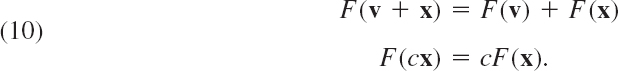
Linear Transformation of Space Rn into Space Rm
From now on we let X = Rn and Y = Rm. Then any real m × n matrix A = [ajk] gives a transformation of Rn into Rm,
![]()
Since A(u + x) = Au + Ax and A(cx) = cAx, this transformation is linear.
We show that, conversely, every linear transformation F of Rn into Rm can be given in terms of an m × n matrix A, after a basis for Rn and a basis for Rm have been chosen. This can be proved as follows.
Let e(1), …, e(n) be any basis for Rn. Then every x in Rn has a unique representation
![]()
Since F is linear, this representation implies for the image F(x):
![]()
Hence F is uniquely determined by the images of the vectors of a basis for Rn. We now choose for Rn the “standard basis”

where e(j) has its jth component equal to 1 and all others 0. We show that we can now determine an m × n matrix A = [ajk] such that for every x in Rn and image y = F(x) in Rm,
![]()
Indeed, from the image y(1) = F(e(1)) of e(1) we get the condition

from which we can determine the first column of A, namely ![]() ,
, ![]() . Similarly, from the image of e(2) we get the second column of A, and so on. This completes the proof.
. Similarly, from the image of e(2) we get the second column of A, and so on. This completes the proof.
We say that A representsF, or is a representation of F, with respect to the bases for Rn and Rm. Quite generally, the purpose of a “representation” is the replacement of one object of study by another object whose properties are more readily apparent.
In three-dimensional Euclidean space E3 the standard basis is usually written e(1) = i, e(2) = j, e(3) = k. Thus,
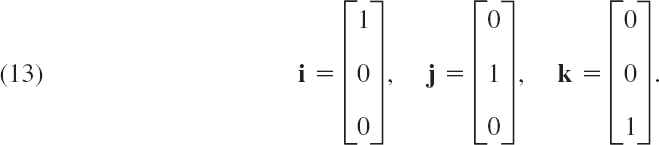
These are the three unit vectors in the positive directions of the axes of the Cartesian coordinate system in space, that is, the usual coordinate system with the same scale of measurement on the three mutually perpendicular coordinate axes.
EXAMPLE 5 Linear Transformations
Interpreted as transformations of Cartesian coordinates in the plane, the matrices
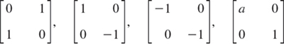
represent a reflection in the line x2 = x1, a reflection in the x1-axis, a reflection in the origin, and a stretch (when a > 1, or a contraction when 0 < a < 1) in the x1-direction, respectively.
EXAMPLE 6 Linear Transformations
Our discussion preceding Example 5 is simpler than it may look at first sight. To see this, find A representing the linear transformation that maps (x1, x2) onto (2x1 − 5x2, 3x1 + 4x2).
Solution. Obviously, the transformation is
![]()
From this we can directly see that the matrix is
![]()
If A in (11) is square, n × n, then (11) maps Rn into Rn. If this A is nonsingular, so that A−1 exists (see Sec. 7.8), then multiplication of (11) by A−1 from the left and use of A−1A = I gives the inverse transformation
![]()
It maps every y = y0 onto that x, which by (11) is mapped onto y0. The inverse of a linear transformation is itself linear, because it is given by a matrix, as (14) shows.
Composition of Linear Transformations
We want to give you a flavor of how linear transformations in general vector spaces work. You will notice, if you read carefully, that definitions and verifications (Example 7) strictly follow the given rules and you can think your way through the material by going in a slow systematic fashion.
The last operation we want to discuss is composition of linear transformations. Let X, Y, W be general vector spaces. As before, let F be a linear transformation from X to Y. Let G be a linear transformation from W to X. Then we denote, by H, the composition of F and G, that is,
![]()
which means we take transformation G and then apply transformation F to it (in that order!, i.e. you go from left to right).
Now, to give this a more concrete meaning, if we let w be a vector in W, then G(w) is a vector in X and F(G(w)) is a vector in Y. Thus, H maps W to Y, and we can write
![]()
which completes the definition of composition in a general vector space setting. But is composition really linear? To check this we have to verify that H, as defined in (15), obeys the two equations of (10).
EXAMPLE 7 The Composition of Linear Transformations Is Linear
To show that H is indeed linear we must show that (10) holds. We have, for two vectors w1, w2 in W,
We defined composition as a linear transformation in a general vector space setting and showed that the composition of linear transformations is indeed linear.
Next we want to relate composition of linear transformations to matrix multiplication.
To do so we let X = Rn, Y = Rm and W = Rp. This choice of particular vector spaces allows us to represent the linear transformations as matrices and form matrix equations, as was done in (11). Thus F can be represented by a general real m × n matrix A = [ajk] and G by an n × p matrix B = [bjk]. Then we can write for F, with column vectors x with n entries, and resulting vector y, with m entries
![]()
and similarly for G, with column vector w with p entries,
![]()
Substituting (17) into (16) gives
![]()
This is (15) in a matrix setting, this is, we can define the composition of linear transformations in the Euclidean spaces as multiplication by matrices. Hence, the real m × p matrix C represents a linear transformation H which maps Rp to Rn with vector w, a column vector with p entries.
Remarks. Our discussion is similar to the one in Sec. 7.2, where we motivated the “unnatural” matrix multiplication of matrices. Look back and see that our current, more general, discussion is written out there for the case of dimension m = 2, n = 2 and p = 2. (You may want to write out our development by picking small distinct dimensions, such as m = 2, n = 3, and p = 4, and writing down the matrices and vectors. This is a trick of the trade of mathematicians in that we like to develop and test theories on smaller examples to see that they work.)
EXAMPLE 8 Linear Transformations. Composition
In Example 5 of Sec. 7.9, let A be the first matrix and B be the fourth matrix with a > 1. Then, applying B to a vector w = [w1 w2]T, stretches the element w1 by a in the x1 direction. Next, when we apply A to the “stretched” vector, we reflect the vector along the line x1 = x2, resulting in a vector y = [w2 aw1]T. But this represents, precisely, a geometric description for the composition H of two linear transformations F and G represented by matrices A and B. We now show that, for this example, our result can be obtained by straightforward matrix multiplication, that is,

and as in (18) calculate
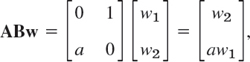
which is the same as before. This shows that indeed AB = C, and we see the composition of linear transformations can be represented by a linear transformation. It also shows that the order of matrix multiplication is important (!). You may want to try applying A first and then B, resulting in BA. What do you see? Does it make geometric sense? Is it the same result as AB?
We have learned several abstract concepts such as vector space, inner product space, and linear transformation. The introduction of such concepts allows engineers and scientists to communicate in a concise and common language. For example, the concept of a vector space encapsulated a lot of ideas in a very concise manner. For the student, learning such concepts provides a foundation for more advanced studies in engineering.
This concludes Chapter 7. The central theme was the Gaussian elimination of Sec. 7.3 from which most of the other concepts and theory flowed. The next chapter again has a central theme, that is, eigenvalue problems, an area very rich in applications such as in engineering, modern physics, and other areas.
- Basis. Find three bases of R2.
- Uniqueness. Show that the representation v = c1a(1) + … + cna(n) of any given vector in an n-dimensional vector space V in terms of a given basis a(1), …, a(n) for V is unique. Hint. Take two representations and consider the difference.
3–10 VECTOR SPACE
(More problems in Problem Set 9.4.) Is the given set, taken with the usual addition and scalar multiplication, a vector space? Give reason. If your answer is yes, find the dimension and a basis.
- 3. All vectors in R3 satisfying −υ1 + 2υ2 + 3υ3 = 0, −4υ1 + υ2 + υ3 = 0.
- 4. All skew-symmetric 3 × 3 matrices.
- 5. All polynomials in x of degree 4 or less with nonnegative coefficients.
- 6. All functions y(x) = a cos 2x + b sin 2x with arbitrary constants a and b.
- 7. All functions y(x) = (ax + b)e−x with any constant a and b.
- 8. All n × n matrices A with fixed n and det A = 0.
- 9. All 2 × 2 matrices [ajk] with a11 + a22 = 0.
- 10. All 3 × 2 matrices [ajk] with first column any multiple of [3 0 −5]T.
11–14 LINEAR TRANSFORMATIONS
Find the inverse transformation. Show the details.
- 11. y1 = 0.5x1 − 0.5x2
y2 = 1.5x1 − 2.5x2
- 12.

- 13.
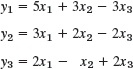
- 14.

15–20 EUCLIDEAN NORM
Find the Euclidean norm of the vectors:
- 15. [3 1 −4]T
- 16.

- 17. [1 0 0 1 −1 0 −1 1]T
- 18. [−4 8 −1]T
- 19.

- 20.

21–25 INNER PRODUCT. ORTHOGONALITY
- 21. Orthogonality. For what value(s) of k are the vectors
 and
and  orthogonal?
 - 22. Orthogonality. Find all vectors in R3 orthogonal to [2 0 1]. Do they form a vector space?
- 23. Triangle inequality. Verify (4) for the vectors in Probs. 15 and 18.
- 24. Cauchy–Schwarz inequality. Verify (3) for the vectors in Probs. 16 and 19.
- 25. Parallelogram equality. Verify (5) for the first two column vectors of the coefficient matrix in Prob. 13.
CHAPTER 7 REVIEW QUESTIONS AND PROBLEMS
- What properties of matrix multiplication differ from those of the multiplication of numbers?
- Let A be a 100 × 100 matrix and B a 100 × 50 matrix. Are the following expressions defined or not? A + B, A2, B2, AB, BA, AAT, BTA, BTB, BTAB. Give reasons.
- Are there any linear systems without solutions? With one solution? With more than one solution? Give simple examples.
- Let C be 10 × 10 matrix and a a column vector with 10 components. Are the following expressions defined or not? Ca, CTa, CaT, aC, aTC, (CaT)T.
- Motivate the definition of matrix multiplication.
- Explain the use of matrices in linear transformations.
- How can you give the rank of a matrix in terms of row vectors? Of column vectors? Of determinants?
- What is the role of rank in connection with solving linear systems?
- What is the idea of Gauss elimination and back substitution?
- What is the inverse of a matrix? When does it exist? How would you determine it?
11–20 MATRIX AND VECTOR CALCULATIONS
Showing the details, calculate the following expressions or give reason why they are not defined, when
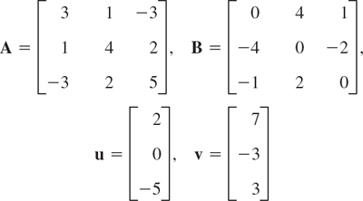
- 11. AB, BA
- 12. AT, BT
- 13. Au, uTA
- 14. uTv, uvT
- 15. uTAu, vTBv
- 16. A−1, B−1
- 17. det A, det A2, (det A)2, det B
- 18. (A2)−1, (A−1)2
- 19. AB − BA
- 20. (A + AT)(B − BT)
21–28 LINEAR SYSTEMS
Showing the details, find all solutions or indicate that no solution exists.
- 21.

- 22.
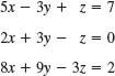
- 23.
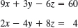
- 24.

- 25.

- 26.
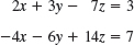
- 27.

- 28.

29–32 RANK
Determine the ranks of the coefficient matrix and the augmented matrix and state how many solutions the linear system will have.
- 29. In Prob. 23
- 30. In Prob. 24
- 31. In Prob. 27
- 32. In Prob. 26
33–35 NETWORKS
Find the currents.
- 33.

- 34.

- 35.
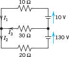
SUMMARY OF CHAPTER 7 Linear Algebra: Matrices, Vectors, Determinants. Linear Systems
An m × n matrix A = [ajk] is a rectangular array of numbers or functions (“entries,” “elements”) arranged in m horizontal rows and n vertical columns. If m = n, the matrix is called square. A 1 × n matrix is called a row vector and an m × 1 matrix a column vector (Sec. 7.1).
The sum A + B of matrices of the same size (i.e., both m × n) is obtained by adding corresponding entries. The product of A by a scalar c is obtained by multiplying each ajk by c (Sec. 7.1).
The product C = AB of an m × n matrix A by an r × p matrix B = [bjk] is defined only when r = n, and is the m × p matrix C = [cjk] with entries

This multiplication is motivated by the composition of linear transformations (Secs. 7.2, 7.9). It is associative, but is not commutative: if AB is defined, BA may not be defined, but even if BA is defined, AB ≠ BA in general. Also AB = 0 may not imply A = 0 or B = 0 or BA = 0 (Secs. 7.2, 7.8). Illustrations:

The transpose AT of a matrix A = [ajk] is AT = [akj]; rows become columns and conversely (Sec. 7.2). Here, A need not be square. If it is and A = AT, then A is called symmetric; if A = −AT, it is called skew-symmetric. For a product, (AB)T = BTAT (Sec. 7.2).
A main application of matrices concerns linear systems of equations
![]()
(m equations in n unknowns x1, …, xn, A and b given). The most important method of solution is the Gauss elimination (Sec. 7.3), which reduces the system to “triangular” form by elementary row operations, which leave the set of solutions unchanged. (Numeric aspects and variants, such as Doolittle's and Cholesky's methods, are discussed in Secs. 20.1 and 20.2.)
Cramer's rule (Secs. 7.6, 7.7) represents the unknowns in a system (2) of n equations in n unknowns as quotients of determinants; for numeric work it is impractical. Determinants (Sec. 7.7) have decreased in importance, but will retain their place in eigenvalue problems, elementary geometry, etc.
The inverse A−1 of a square matrix satisfies AA−1 = A−1A = I. It exists if det A ≠ 0. It can be computed by the Gauss–Jordan elimination (Sec. 7.8).
The rank r of a matrix A is the maximum number of linearly independent rows or columns of A or, equivalently, the number of rows of the largest square submatrix of A with nonzero determinant (Secs. 7.4, 7.7).
The system (2) has solutions if and only if rank A = rank [A b], where [A b] is the augmented matrix (Fundamental Theorem, Sec. 7.5).
The homogeneous system
![]()
has solutions x ≠ 0 (“nontrivial solutions”) if and only if rank A < n, in the case m = n equivalently if and only if det A = 0 (Secs. 7.6, 7.7).
Vector spaces, inner product spaces, and linear transformations are discussed in Sec. 7.9. See also Sec. 7.4.
1ANDREI ANDREJEVITCH MARKOV (1856–1922), Russian mathematician, known for his work in probability theory.
2GABRIEL CRAMER (1704–1752), Swiss mathematician.
3WILHELM JORDAN (1842–1899), German geodesist and mathematician. He did important geodesic work in Africa, where he surveyed oases. [See Althoen, S.C. and R. McLaughlin, Gauss–Jordan reduction: A brief history. American Mathematical Monthly, Vol. 94, No. 2 (1987), pp. 130–142.]
We do not recommend it as a method for solving systems of linear equations, since the number of operations in addition to those of the Gauss elimination is larger than that for back substitution, which the Gauss–Jordan elimination avoids. See also Sec. 20.1.
4DAVID HILBERT (1862–1943), great German mathematician, taught at Königsberg and Göttingen and was the creator of the famous Göttingen mathematical school. He is known for his basic work in algebra, the calculus of variations, integral equations, functional analysis, and mathematical logic. His “Foundations of Geometry” helped the axiomatic method to gain general recognition. His famous 23 problems (presented in 1900 at the International Congress of Mathematicians in Paris) considerably influenced the development of modern mathematics.
If V is finite dimensional, it is actually a so-called Hilbert space; see [GenRef7], p. 128, listed in App. 1.
5HERMANN AMANDUS SCHWARZ (1843–1921). German mathematician, known by his work in complex analysis (conformal mapping) and differential geometry. For Cauchy see Sec. 2.5.