
CHAPTER 4
Systems of ODEs. Phase Plane. Qualitative Methods

Tying in with Chap. 3, we present another method of solving higher order ODEs in Sec. 4.1. This converts any nth-order ODE into a system of n first-order ODEs. We also show some applications. Moreover, in the same section we solve systems of first-order ODEs that occur directly in applications, that is, not derived from an nth-order ODE but dictated by the application such as two tanks in mixing problems and two circuits in electrical networks. (The elementary aspects of vectors and matrices needed in this chapter are reviewed in Sec. 4.0 and are probably familiar to most students.)
In Sec. 4.3 we introduce a totally different way of looking at systems of ODEs. The method consists of examining the general behavior of whole families of solutions of ODEs in the phase plane, and aptly is called the phase plane method. It gives information on the stability of solutions. (Stability of a physical system is desirable and means roughly that a small change at some instant causes only a small change in the behavior of the system at later times.) This approach to systems of ODEs is a qualitative method because it depends only on the nature of the ODEs and does not require the actual solutions. This can be very useful because it is often difficult or even impossible to solve systems of ODEs. In contrast, the approach of actually solving a system is known as a quantitative method.
The phase plane method has many applications in control theory, circuit theory, population dynamics and so on. Its use in linear systems is discussed in Secs. 4.3, 4.4, and 4.6 and its even more important use in nonlinear systems is discussed in Sec. 4.5 with applications to the pendulum equation and the Lokta–Volterra population model. The chapter closes with a discussion of nonhomogeneous linear systems of ODEs.
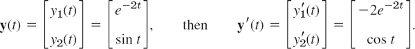
NOTATION. We continue to denote unknown functions by y; thus, y1(t), y2(t)—analogous to Chaps. 1–3. (Note that some authors use x for functions, x1(t), x2(t) when dealing with systems of ODEs.)
Prerequisite: Chap. 2.
References and Answers to Problems: App. 1 Part A, and App. 2.
4.0 For Reference: Basics of Matrices and Vectors
For clarity and simplicity of notation, we use matrices and vectors in our discussion of linear systems of ODEs. We need only a few elementary facts (and not the bulk of the material of Chaps. 7 and 8). Most students will very likely be already familiar with these facts. Thus this section is for reference only. Begin with Sec. 4.1 and consult4.0 as needed.
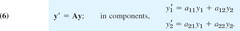
Most of our linear systems will consist of two linear ODEs in two unknown functions y1(t), y2(t)

(perhaps with additional given functions g1(t), g2(t) on the right in the two ODEs).
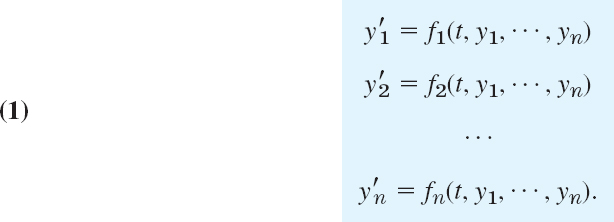
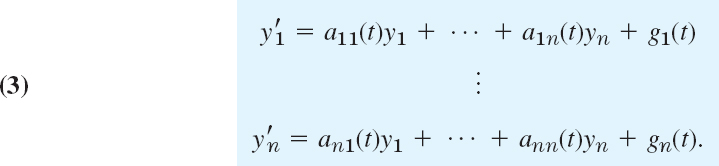
Similarly, a linear system of n first-order ODEs in n unknown functions y1(t), …, yn(t) is of the form

(perhaps with an additional given function on the right in each ODE).
Some Definitions and Terms
Matrices. In (1) the (constant or variable) coefficients form a 2 × 2 matrix A, that is, an array

Similarly, the coefficients in (2) form an n × n matrix
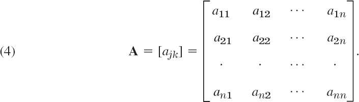
The a11, a12, … are called entries, the horizontal lines rows, and the vertical lines columns. Thus, in (3) the first row is [a11 a12], the second row is [a21 a22], and the first and second columns are

In the “double subscript notation” for entries, the first subscript denotes the row and the second the column in which the entry stands. Similarly in (4). The main diagonal is the diagonal a11 a22 … ann in (4), hence a11 a22 in (3).
We shall need only square matrices, that is, matrices with the same number of rows and columns, as in (3) and (4).
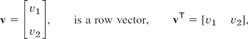
Vectors. A column vector x with n components x1, …, xn is of the form
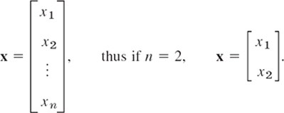
Similarly, a row vector v is of the form
![]()
Calculations with Matrices and Vectors
Equality. Two n × n matrices are equal if and only if corresponding entries are equal. Thus for n = 2, let
Then A = B if and only if

Two column vectors (or two row vectors) are equal if and only if they both have n components and corresponding components are equal. Thus, let
Addition is performed by adding corresponding entries (or components); here, matrices must both be n × n, and vectors must both have the same number of components. Thus for n = 2,

Scalar multiplication (multiplication by a number c) is performed by multiplying each entry (or component) by c. For example, if


Matrix Multiplication. The product C = AB (in this order) of two n × n matrices A = [ajk] and B = [bjk] is the n × n matrix C = [cjk] with entries

that is, multiply each entry in the jth row of A by the corresponding entry in the kth column of B and then add these n products. One says briefly that this is a “multiplication of rows into columns.” For example,

CAUTION! Matrix multiplication is not commutative, AB ≠ BA in general. In our example,

Multiplication of an n × n matrix A by a vector x with n components is defined by the same rule: v = Ax is the vector with the n components

For example,

Systems of ODEs as Vector Equations
Differentiation. The derivative of a matrix (or vector) with variable entries (or components) is obtained by differentiating each entry (or component). Thus, if
Using matrix multiplication and differentiation, we can now write (1) as
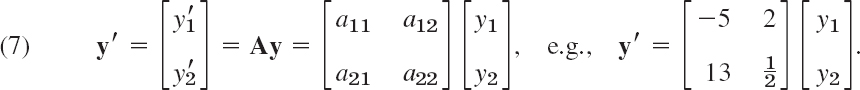
Similarly for (2) by means of an n × n matrix A and a column vector y with n components, namely, y′ = Ay. The vector equation (7) is equivalent to two equations for the components, and these are precisely the two ODEs in (1).
Some Further Operations and Terms
Transposition is the operation of writing columns as rows and conversely and is indicated by T. Thus the transpose AT of the 2 × 2 matrix

The transpose of a column vector, say,
and conversely.
Inverse of a Matrix. The n × n unit matrix I is the n × n matrix with main diagonal 1, 1, …, 1 and all other entries zero. If, for a given n × n matrix A, there is an n × n matrix B such that AB = BA = I, thenA is called nonsingular and B is called the inverse of A and is denoted by A−1; thus
![]()
The inverse exists if the determinant det A of A is not zero.
If A has no inverse, it is called singular. For n = 2,

where the determinant of A is

(For general n, see Sec. 7.7, but this will not be needed in this chapter.)
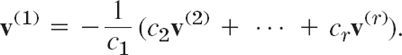
Linear Independence. r given vectors v(1), …, v(r) with n components are called a linearly independent set or, more briefly, linearly independent, if
![]()
implies that all scalars c1, …, cr must be zero; here, 0 denotes the zero vector, whose n components are all zero. If (11) also holds for scalars not all zero (so that at least one of these scalars is not zero), then these vectors are called a linearly dependent set or, briefly, linearly dependent, because then at least one of them can be expressed as a linear combination of the others; that is, if, for instance, c1 ≠ 0 in (11), then we can obtain
Eigenvalues, Eigenvectors
Eigenvalues and eigenvectors will be very important in this chapter (and, as a matter of fact, throughout mathematics).
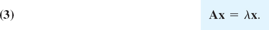
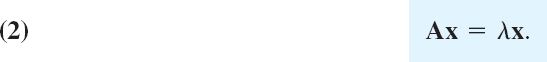
Let A = [ajk] be an n × n matrix. Consider the equation

where λ is a scalar (a real or complex number) to be determined and x is a vector to be determined. Now, for every λ, a solution is x = 0. A scalar λ such that (12) holds for some vector x ≠ 0 is called an eigenvalue of A, and this vector is called an eigenvector of A corresponding to this eigenvalue λ.
We can write (12) as Ax − λx = 0 or
![]()
These are n linear algebraic equations in the n unknowns x1, …, xn (the components of x). For these equations to have a solution x ≠ 0, the determinant of the coefficient matrix A − λI must be zero. This is proved as a basic fact in linear algebra (Theorem 4 in Sec. 7.7). In this chapter we need this only for n = 2. Then (13) is
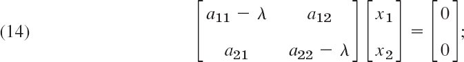
in components,
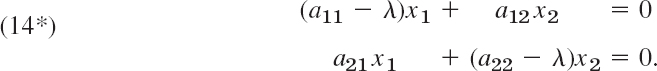
Now A − λI is singular if and only if its determinant dt (A − λI), called the characteristic determinant of A (also for general n), is zero. This gives
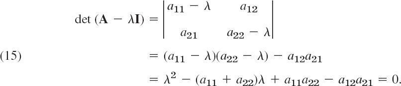
This quadratic equation in λ is called the characteristic equation of A. Its solutions are the eigenvalues λ1 and λ2 of A. First determine these. Then use (14*) with λ = λ1 to determine an eigenvector x(1) of A corresponding to λ1. Finally use (14*) with λ = λ2 to find an eigenvector x(2) of A corresponding to λ2. Note that if x is an eigenvector of A, so is kx with any k ≠ 0.
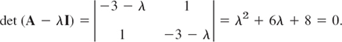
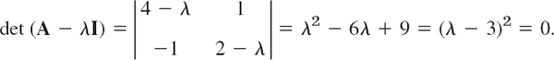
Find the eigenvalues and eigenvectors of the matrix
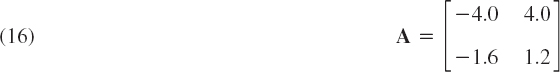
Solution. The characteristic equation is the quadratic equation

It has the solutions λ1 = −2 and λ2 = −0.8. These are the eigenvalues of A.
Eigenvectors are obtained from (14*). For λ = λ1 = −2 we have from (14*)
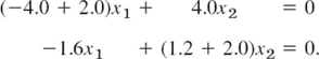
A solution of the first equation is x1 = 2, x2 = 1. This also satisfies the second equation. (Why?) Hence an eigenvector of A corresponding to λ1 = −2.0 is
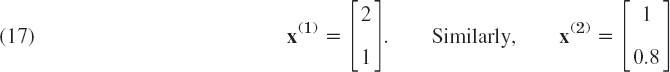
is an eigenvector of A corresponding to λ2 = −0.8, as obtained from (14*) with λ = λ2. Verify this.
4.1 Systems of ODEs as Models in Engineering Applications
We show how systems of ODEs are of practical importance as follows. We first illustrate how systems of ODEs can serve as models in various applications. Then we show how a higher order ODE (with the highest derivative standing alone on one side) can be reduced to a first-order system.
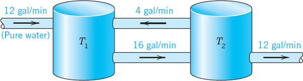
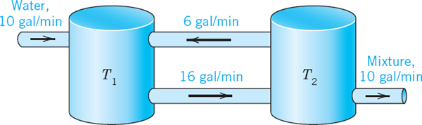
EXAMPLE 1 Mixing Problem Involving Two Tanks
A mixing problem involving a single tank is modeled by a single ODE, and you may first review the corresponding Example 3 in Sec. 1.3 because the principle of modeling will be the same for two tanks. The model will be a system of two first-order ODEs.
Tank T1 and T2 in Fig. 78 contain initially 100 gal of water each. In T1 the water is pure, whereas 150 lb of fertilizer are dissolved in T2. By circulating liquid at a rate of 2 gal/min and stirring (to keep the mixture uniform) the amounts of fertilizer y1(t) in T1 and y2(t) in T2 change with time t. How long should we let the liquid circulate so that T1 will contain at least half as much fertilizer as there will be left in T2?
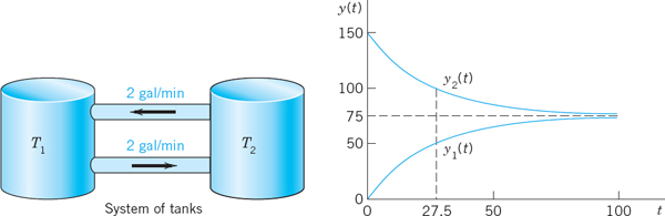
Fig. 78. Fertilizer content in Tanks (lower curve) and T2
Solution. Step 1. Setting up the model. As for a single tank, the time rate of change y′1(t) of y1(t) equals inflow minus outflow. Similarly for tank T2. From Fig. 78 we see that

Hence the mathematical model of our mixture problem is the system of first-order ODEs

As a vector equation with column vector ![]() and matrix A this becomes
and matrix A this becomes

Step 2. General solution. As for a single equation, we try an exponential function of t,

Dividing the last equation λxeλt = Axeλt by eλt and interchanging the left and right sides, we obtain
![]()
We need nontrivial solutions (solutions that are not identically zero). Hence we have to look for eigenvalues and eigenvectors of A. The eigenvalues are the solutions of the characteristic equation
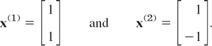
We see that λ1 = 0 (which can very well happen—don't get mixed up—it is eigen vectors that must not be zero) and λ2 = −0.04. Eigenvectors are obtained from (14*) in Sec. 4.0 with λ = 0 and λ = −0.04. For our present A this gives [we need only the first equation in (14*)]
![]()
respectively. Hence x1 = x2 and x1 = −x2, respectively, and we can take x1 = x2 = 1 and x1 = −x2 = 1. This gives two eigenvectors corresponding to λ1 = 0 and λ2 = −0.04, respectively, namely,
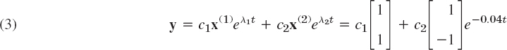
From (1) and the superposition principle (which continues to hold for systems of homogeneous linear ODEs) we thus obtain a solution
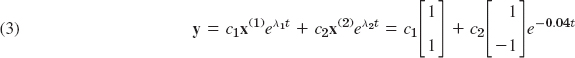
where c1 are c2 arbitrary constants. Later we shall call this a general solution.
Step 3. Use of initial conditions. The initial conditions are y1(0) = 0 (no fertilizer in tank T1) and y2(0) = 150. From this and (3) with t = 0 we obtain
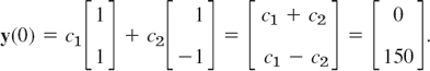
In components this is c1 + c2 = 0, c1 − c2 = 150. The solution is c1 = 75, c2 = −75. This gives the answer
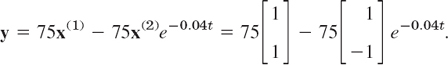
In components,

Figure 78 shows the exponential increase of y1 and the exponential decrease of y2 to the common limit 75 lb. Did you expect this for physical reasons? Can you physically explain why the curves look “symmetric”? Would the limit change if T1 initially contained 100 lb of fertilizer and T2 contained 50 lb?
Step 4. Answer. T1 contains half the fertilizer amount of T2 if it contains 1/3 of the total amount, that is, 50 lb. Thus
![]()
Hence the fluid should circulate for at least about half an hour.
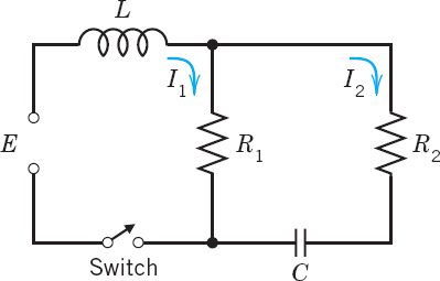
Find the currents I1(t) and I2(t) in the network in Fig. 79. Assume all currents and charges to be zero at t = 0, the instant when the switch is closed.
Fig. 79. Electrical network in Example 2
Solution. Step 1. Setting up the mathematical model. The model of this network is obtained from Kirchhoff's Voltage Law, as in Sec. 2.9 (where we considered single circuits). Let I1(t) and I2(t) be the currents in the left and right loops, respectively. In the left loop, the voltage drops are LI′1 = I′1 [V] over the inductor and R1(I1 − I2) = 4(I1 − I2)[V] over the resistor, the difference because I1 and I2 flow through the resistor in opposite directions. By Kirchhoff's Voltage Law the sum of these drops equals the voltage of the battery; that is, I′1 + 4(I1 − I2) = 12, hence
![]()
In the right loop, the voltage drops are R2I2 = 6I2[V] and R1(I2 − I1) = 4(I2 − I1)[V] over the resistors and (I/C)∫ I2 dt = 4 ∫ I2 dt[V] over the capacitor, and their sum is zero,
![]()
Division by 10 and differentiation gives I′2 − 0.4I′1 + 0.4I2 = 0.
To simplify the solution process, we first get rid of 0.4I′1, which by (4a) equals 0.4(−4I1 + 4I2 + 12). Substitution into the present ODE gives
![]()
and by simplification
![]()
In matrix form, (4) is (we write J since I is the unit matrix)

Step 2. Solving (5). Because of the vector g this is a nonhomogeneous system, and we try to proceed as for a single ODE, solving first the homogeneous system J′ = AJ (thus J′ − AJ = 0) by substituting J = xeλt. This gives
![]()
Hence, to obtain a nontrivial solution, we again need the eigenvalues and eigenvectors. For the present matrix A they are derived in Example 1 in Sec. 4.0:

Hence a “general solution” of the homogeneous system is
![]()
For a particular solution of the nonhomogeneous system (5), since g is constant, we try a constant column vector Jp = a with components a1, a2. Then J′p = 0, and substitution into (5) gives Aa + g = 0; in components,

The solution is a1 = 3, a2 = 0; thus ![]() . Hence
. Hence
![]()
in components,


Hence c1 = −4 and c2 = 5. As the solution of our problem we thus obtain
![]()
In components (Fig. 80b),
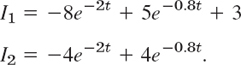
Now comes an important idea, on which we shall elaborate further, beginning in Sec. 4.3. Figure 80a shows I1(t) and I2(t) as two separate curves. Figure 80b shows these two currents as a single curve [I1(t), I2(t)] in the I1I2-plane. This is a parametric representation with time t as the parameter. It is often important to know in which sense such a curve is traced. This can be indicated by an arrow in the sense of increasing t, as is shown. The I1I2-plane is called the phase plane of our system (5), and the curve in Fig. 80b is called a trajectory. We shall see that such “phase plane representations” are far more important than graphs as in Fig. 80a because they will give a much better qualitative overall impression of the general behavior of whole families of solutions, not merely of one solution as in the present case.
Fig. 80. Currents in Example 2
Remark. In both examples, by growing the dimension of the problem (from one tank to two tanks or one circuit to two circuits) we also increased the number of ODEs (from one ODE to two ODEs). This “growth” in the problem being reflected by an “increase” in the mathematical model is attractive and affirms the quality of our mathematical modeling and theory.
Conversion of an nth-Order ODE to a System
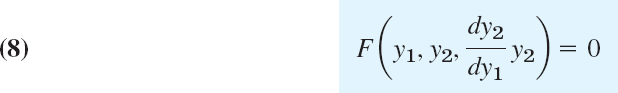
We show that an nth-order ODE of the general form (8) (see Theorem 1) can be converted to a system of n first-order ODEs. This is practically and theoretically important—practically because it permits the study and solution of single ODEs by methods for systems, and theoretically because it opens a way of including the theory of higher order ODEs into that of first-order systems. This conversion is another reason for the importance of systems, in addition to their use as models in various basic applications. The idea of the conversion is simple and straightforward, as follows.
THEOREM 1 Conversion of an ODE
An nth-order ODE
![]()
can be converted to a system of n first-order ODEs by setting

This system is of the form

PROOF
The first n − 1 of these n ODEs follows immediately from (9) by differentiation. Also, y′n = y(n) by (9), so that the last equation in (10) results from the given ODE (8).
To gain confidence in the conversion method, let us apply it to an old friend of ours, modeling the free motions of a mass on a spring (see Sec. 2.4)
![]()
For this ODE (8) the system (10) is linear and homogeneous,

Setting ![]() , we get in matrix form
, we get in matrix form
The characteristic equation is

It agrees with that in Sec. 2.4. For an illustrative computation, let m = 1, c = 2, and k = 0.75. Then
![]()
This gives the eigenvalues λ1 = −0.5 and λ2 = −1.5. Eigenvectors follow from the first equation in A − λI = 0, which is −λx1 + x2 = 0. For λ1 this gives 0.5x1 + x2 = 0, say, x1 = 2, x2 = −1. For λ2 = −1.5 it gives 1.5x1 + x2 = 0, say, x1 = 1, x2 = −1.5. These eigenvectors

This vector solution has the first component
![]()
which is the expected solution. The second component is its derivative
![]()
1–6 MIXING PROBLEMS
- Find out, without calculation, whether doubling the flow rate in Example 1 has the same effect as halfing the tank sizes. (Give a reason.)
- What happens in Example 1 if we replace T1 by a tank containing 200 gal of water and 150 lb of fertilizer dissolved in it?
- Derive the eigenvectors in Example 1 without consulting this book.
- In Example 1 find a “general solution” for any ratio a = (flow rate)/(tank size), tank sizes being equal. Comment on the result.
- If you extend Example 1 by a tank T3 of the same size as the others and connected to T2 by two tubes with flow rates as between T1 and T2, what system of ODEs will you get?
- Find a “general solution” of the system in Prob. 5.
7–9 ELECTRICAL NETWORK
In Example 2 find the currents:
- 7. If the initial currents are 0 A and −3 A (minus meaning that I2(0) flows against the direction of the arrow).
- 8. If the capacitance is changed to C = 5/27 F. (General solution only.)
- 9. If the initial currents in Example 2 are 28 A and 14 A.
10–13 CONVERSION TO SYSTEMS
Find a general solution of the given ODE (a) by first converting it to a system, (b), as given. Show the details of your work.
- 10. y″ + 3y′ + 2y = 0
- 11. 4y″ − 15y′ − 4y = 0
- 12. y″′ + 2y″ − y′ − 2y = 0
- 13. y″ + 2y′ − 24y = 0
- 14. TEAM PROJECT. Two Masses on Springs. (a) Set up the model for the (undamped) system in Fig. 81. (b) Solve the system of ODEs obtained. Hint. Try y = xeωt and set ω2 = λ. Proceed as in Example 1 or 2. (c) Describe the influence of initial conditions on the possible kind of motions.

- 15. CAS EXPERIMENT. Electrical Network. (a) In Example 2 choose a sequence of values of C that increases beyond bound, and compare the corresponding sequences of eigenvalues of A. What limits of these sequences do your numeric values (approximately) suggest?
(b) Find these limits analytically.
(c) Explain your result physically.
(d) Below what value (approximately) must you decrease C to get vibrations?
4.2 Basic Theory of Systems of ODEs. Wronskian
In this section we discuss some basic concepts and facts about system of ODEs that are quite similar to those for single ODEs.
The first-order systems in the last section were special cases of the more general system
We can write the system (1) as a vector equation by introducing the column vectors y = [y1 … yn]T and f = [f1 … fn]T (where T means transposition and saves us the space that would be needed for writing y and f as columns). This gives

This system (1) includes almost all cases of practical interest. For n = 1 it becomes y′1 = f1(t, y1) or, simply, y′ = f(t, y), well known to us from Chap. 1.
A solution of (1) on some interval a < t < b is a set of n differentiable functions
![]()
on a < t < b that satisfy (1) throughout this interval. In vector from, introducing the “solution vector” h = [h1 … hn]T (a column vector!) we can write
![]()
An initial value problem for (1) consists of (1) and n given initial conditions
![]()
in vector form, y(t0) = K, where t0 is a specified value of t in the interval considered and the components of K = [K1 … Kn]T are given numbers. Sufficient conditions for the existence and uniqueness of a solution of an initial value problem (1), (2) are stated in the following theorem, which extends the theorems in Sec. 1.7 for a single equation. (For a proof, see Ref. [A7].)
THEOREM 1 Existence and Uniqueness Theorem
Let f1 …, fn in (1) be continuous functions having continuous partial derivatives ∂f1/∂y1, …, ∂f1/∂yn, …, ∂fn/∂yn in some domain R of ty1y2 … yn-space containing the point (t0, K1, … Kn). Then (1) has a solution on some interval t0 − α < t < t0 + α satisfying (2) , and this solution is unique.
Linear Systems
Extending the notion of a linear ODE, we call (1) a linear system if it is linear in y1, …, yn; that is, if it can be written
As a vector equation this becomes

where 
This system is called homogeneous if g = 0, so that it is
![]()
If g ≠ 0, then (3) is called nonhomogeneous. For example, the systems in Examples 1 and 3 of Sec. 4.1 are homogeneous. The system in Example 2 of that section is nonhomogeneous.
For a linear system (3) we have ∂f1/∂y1 = a11(t), …, ∂fn/∂fn = ann(t) in Theorem 1. Hence for a linear system we simply obtain the following.
THEOREM 2 Existence and Uniqueness in the Linear Case
Let the ajk's and gj's in (3) be continuous functions of t on an open interval α < t < β containing the point t = t0. Then (3) has a solution y(t) on this interval satisfying (2) , and this solution is unique.
As for a single homogeneous linear ODE we have
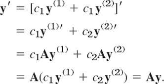
THEOREM 3 Superposition Principle or Linearity Principle
If y(1) and y(2) are solutions of the homogeneous linear system (4) on some interval, so is any linear combination y = c1y(1) + c1y(2).
PROOF
Differentiating and using (4), we obtain
The general theory of linear systems of ODEs is quite similar to that of a single linear ODE in Secs. 2.6 and 2.7. To see this, we explain the most basic concepts and facts. For proofs we refer to more advanced texts, such as [A7].
Basis. General Solution. Wronskian
By a basis or a fundamental system of solutions of the homogeneous system (4) on some interval J we mean a linearly independent set of n solutions y(1), …, y(n) of (4) on that interval. (We write J because we need I to denote the unit matrix.) We call a corresponding linear combination

a general solution of (4) on J. It can be shown that if the ajk(t) in (4) are continuous on J, then (4) has a basis of solutions on J, hence a general solution, which includes every solution of (4) on J.
We can write n solutions y(1), …, y(n) of (4) on some interval J as columns of an n × n matrix
![]()
The determinant of Y is called the Wronskian of y(1), …, y(n), written

The columns are these solutions, each in terms of components. These solutions form a basis on J if and only if W is not zero at any t1 in this interval. W is either identically zero or nowhere zero in J. (This is similar to Secs. 2.6 and 3.1.)
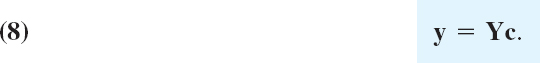
If the solutions y(1), … y(n) in (5) form a basis (a fundamental system), then (6) is often called a fundamental matrix. Introducing a column vector c = [c1 c2 … cn]T, we can now write (5) simply as
Furthermore, we can relate (7) to Sec. 2.6, as follows. If y and z are solutions of a second-order homogeneous linear ODE, their Wronskian is

To write this ODE as a system, we have to set y = y1, y′ = y′1 = y2 and similarly for z (see Sec. 4.1). But then W(y, z) becomes (7), except for notation.
4.3 Constant-Coefficient Systems. Phase Plane Method
Continuing, we now assume that our homogeneous linear system

under discussion has constant coefficients, so that the n × n matrix A = [ajk] has entries not depending on t. We want to solve (1). Now a single ODE y′ = ky has the solution y = Cekt. So let us try
![]()
Substitution into (1) gives y′ = λxeλt = Ay = Axeλt. Dividing by eλt, we obtain the eigenvalue problem
Thus the nontrivial solutions of (1) (solutions that are not zero vectors) are of the form (2), where λ is an eigenvalue of A and x is a corresponding eigenvector.
We assume that A has a linearly independent set of n eigenvectors. This holds in most applications, in particular if A is symmetric (akj = ajk) or skew-symmetric (akj = −ajk) or has n different eigenvalues.
Let those eigenvectors be x(1), …, x(n) and let them correspond to eigenvalues λ1, …, λn (which may be all different, or some—or even all—may be equal). Then the corresponding solutions (2) are

Their Wronskian W = W(y(1), …, y(n)) [(7) in Sec. 4.2] is given by

On the right, the exponential function is never zero, and the determinant is not zero either because its columns are the n linearly independent eigenvectors. This proves the following theorem, whose assumption is true if the matrix A is symmetric or skew-symmetric, or if the n eigenvalues of A are all different.
If the constant matrix A in the system (1) has a linearly independent set of n eigenvectors, then the corresponding solutions y(1), …, y(n) in (4) form a basis of solutions of (1) , and the corresponding general solution is

How to Graph Solutions in the Phase Plane
We shall now concentrate on systems (1) with constant coefficients consisting of two ODEs
Of course, we can graph solutions of (6),

as two curves over the t-axis, one for each component of y(t). (Figure 80a in Sec. 4.1 shows an example.) But we can also graph (7) as a single curve in the y1y2-plane. This is a parametric representation (parametric equation) with parameter t. (See Fig. 80b for an example. Many more follow. Parametric equations also occur in calculus.) Such a curve is called a trajectory (or sometimes an orbit or path) of (6). The y1y2-plane is called the phase plane.1 If we fill the phase plane with trajectories of (6), we obtain the so-called phase portrait of (6).
Studies of solutions in the phase plane have become quite important, along with advances in computer graphics, because a phase portrait gives a good general qualitative impression of the entire family of solutions. Consider the following example, in which we develop such a phase portrait.
EXAMPLE 1 Trajectories in the Phase Plane (Phase Portrait)
Find and graph solutions of the system.
In order to see what is going on, let us find and graph solutions of the system

Solution. By substituting y = xeλt and y′ and y′ = λxeλt dropping the exponential function we get Ax = λx. The characteristic equation is
This gives the eigenvalues λ1 = −2 and λ2 = −4. Eigenvectors are then obtained from
![]()
For λ1 = −2 this is −x1 + x2 = 0. Hence we can take x(1) = [1 1]T. For λ2 = −4 this becomes x1 + x2 = 0, and an eigenvector is x(2) = [1 −1]T. This gives the general solution
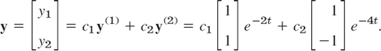
Figure 82 shows a phase portrait of some of the trajectories (to which more trajectories could be added if so desired). The two straight trajectories correspond to c1 = 0 and c2 = 0 and the others to other choices of c1, c2.
The method of the phase plane is particularly valuable in the frequent cases when solving an ODE or a system is inconvenient of impossible.
Critical Points of the System (6)
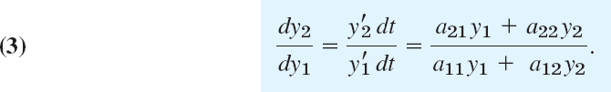
The point y = 0 in Fig. 82 seems to be a common point of all trajectories, and we want to explore the reason for this remarkable observation. The answer will follow by calculus. Indeed, from (6) we obtain
This associates with every point P: (y1, y2) a unique tangent direction dy2/dy1 of the trajectory passing through P, except for the point P = P0: (0, 0), where the right side of (9) becomes 0/0. This point P0, at which dy2/dy1 becomes undetermined, is called a critical point of (6).
Five Types of Critical Points
There are five types of critical points depending on the geometric shape of the trajectories near them. They are called improper nodes, proper nodes, saddle points, centers, and spiral points. We define and illustrate them in Examples 1–5.
EXAMPLE 1 (Continued) Improper Node (Fig. 82)
An improper node is a critical point P0 at which all the trajectories, except for two of them, have the same limiting direction of the tangent. The two exceptional trajectories also have a limiting direction of the tangent at P0 which, however, is different.
The system (8) has an improper node at 0, as its phase portrait Fig. 82 shows. The common limiting direction at 0 is that of the eigenvector x(1) = [1 1]T because e−4t goes to zero faster than e−2t as t increases. The two exceptional limiting tangent directions are those of x(2) = [1 −1]T and −x(2) = [−1 1]T.
EXAMPLE 2 Proper Node (Fig. 83)
A proper node is a critical point P0 at which every trajectory has a definite limiting direction and for any given direction d at P0 there is a trajectory having d as its limiting direction.
The system

has a proper node at the origin (see Fig. 83). Indeed, the matrix is the unit matrix. Its characteristic equation (1 − λ)2 = 0 has the root λ = 1. Any x ≠ 0 is an eigenvector, and we can take [1 0]T and [0 1]T. Hence a general solution is
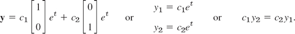

Fig. 82. Trajectories of the system (8) (Improper node)
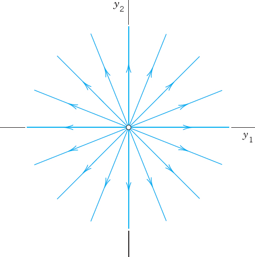
Fig. 83. Trajectories of the system (10) (Proper node)
EXAMPLE 3 Saddle Point (Fig. 84)
A saddle point is a critical point P0 at which there are two incoming trajectories, two outgoing trajectories, and all the other trajectories in a neighborhood of P0 bypass P0.
The system
has a saddle point at the origin. Its characteristic equation (1 − λ)(−1 − λ) = 0 has the roots λ1 = 1 and λ2 = −1. For λ = 1 an eigenvector [1 0]T is obtained from the second row of (A − λI)x = 0, that is, 0x1 + (−1 − 1)x2 = 0. For λ2 = −1 the first row gives [0 1]T. Hence a general solution is
This is a family of hyperbolas (and the coordinate axes); see Fig. 84.
EXAMPLE 4 Center (Fig. 85)
A center is a critical point that is enclosed by infinitely many closed trajectories.
The system

has a center at the origin. The characteristic equation λ2 + 4 = 0 gives the eigenvalues 2i and −2i. For 2i an eigenvector follows from the first equation of −2ix1 + x2 = 0 of (A − λI)x = 0, say, [1 2i]T. For λ = −2i that equation is −(−2i)x1 + x2 = 0 and gives, say, [1 −2i]T. Hence a complex general solution is

A real solution is obtained from (12*) by the Euler formula or directly from (12) by a trick. (Remember the trick and call it a method when you apply it again.) Namely, the left side of (a) times the right side of (b) is −4y1y′1. This must equal the left side of (b) times the right side of (a). Thus,
![]()
This is a family of ellipses (see Fig. 85) enclosing the center at the origin.
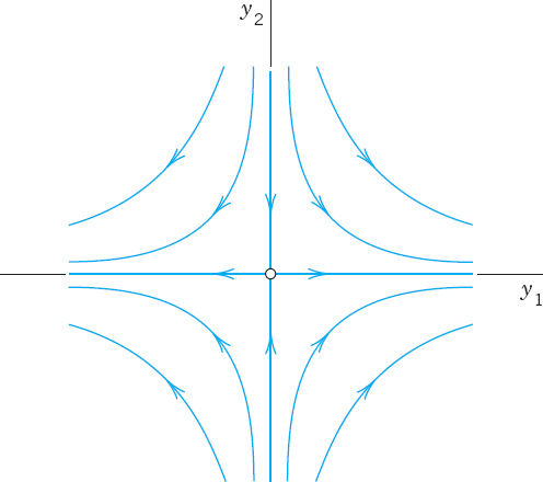
Fig. 84. Trajectories of the system (11) (Saddle point)
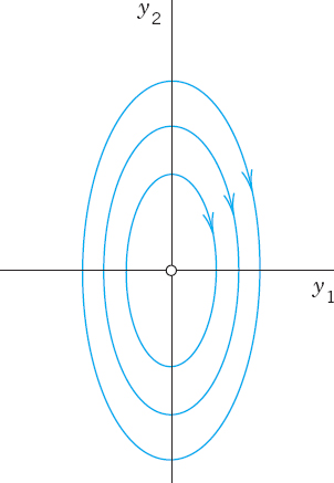
Fig. 85. Trajectories of the system (12) (Center)
EXAMPLE 5 Spiral Point (Fig. 86)
A spiral point is a critical point P0 about which the trajectories spiral, approaching P0 as t → ∞ (or tracing these spirals in the opposite sense, away from P0).
The system

has a spiral point at the origin, as we shall see. The characteristic equation is λ2 + 2λ + 2 = 0. It gives the eigenvalues −1 + i and −1 − i. Corresponding eigenvectors are obtained from (−1 − λ)x1 + x2 = 0. For λ = −1 + i this becomes −ix1 + x2 = 0 and we can take [1 i]T as an eigenvector. Similarly, an eigenvector corresponding to −1 − i is [1 −i]T. This gives the complex general solution

The next step would be the transformation of this complex solution to a real general solution by the Euler formula. But, as in the last example, we just wanted to see what eigenvalues to expect in the case of a spiral point. Accordingly, we start again from the beginning and instead of that rather lengthy systematic calculation we use a shortcut. We multiply the first equation in (13) by y1, the second by y2, and add, obtaining
![]()
We now introduce polar coordinates r, t, where ![]() . Differentiating this with respect to t gives 2rr′ = 2y1y′1 + 2y2y′2. Hence the previous equation can be written
. Differentiating this with respect to t gives 2rr′ = 2y1y′1 + 2y2y′2. Hence the previous equation can be written
![]()
For each real c this is a spiral, as claimed (see Fig. 86).

Fig. 86. Trajectories of the system (13) (Spiral point)
EXAMPLE 6 No Basis of Eigenvectors Available. Degenerate Node (Fig. 87)
This cannot happen if A in (1) is symmetric (akj = ajk, as in Examples 1–3) or skew-symmetric (akj = −ajk, thus ajj = 0). And it does not happen in many other cases (see Examples 4 and 5). Hence it suffices to explain the method to be used by an example.
Find and graph a general solution of

Solution. A is not skew-symmetric! Its characteristic equation is
It has a double root λ = 3. Hence eigenvectors are obtained from (4 − λ)x1 + x2 = 0, thus from x1 + x2 = 0, say, x(1) = [1 −1]T and nonzero multiples of it (which do not help). The method now is to substitute

with constant u = [u1 u2]T into (14). (The xt-term alone, the analog of what we did in Sec. 2.2 in the case of a double root, would not be enough. Try it.) This gives
![]()
On the right, Ax = λx. Hence the terms λxteλt cancel, and then division by eλt gives
![]()
Here λ = 3 and x = [1 −1]T, so that
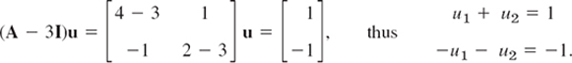
A solution, linearly independent of x = [1 −1]T, is u = [0 1]T. This yields the answer (Fig. 87)

The critical point at the origin is often called a degenerate node. c1y(1) gives the heavy straight line, with c1 > 0 the lower part and c1 < 0 the upper part of it. y(2) gives the right part of the heavy curve from 0 through the second, first, and—finally—fourth quadrants. −y(2) gives the other part of that curve.

Fig. 87. Degenerate node in Example 6
We mention that for a system (1) with three or more equations and a triple eigenvalue with only one linearly independent eigenvector, one will get two solutions, as just discussed, and a third linearly independent one from
![]()
1–9 GENERAL SOLUTION
Find a real general solution of the following systems. Show the details.
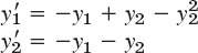
- y′1 = y1 + y2
y′2 = 3y1 − y2
- y′1 = 6y1 + 9y2
y′2 = y1 + 6y2
- y′1 = y1 + 2y2

- y′1 = −8y1 − 2y2
y′2 = 2y1 − 4y2
- y′1 = 2y1 + 5y2
y′2 = 5y1 + 12.5y2
- y′1 = 2y1 − 2y2
y′2 = 2y1 + 2y2
- y′1 = y2
y′2 = −y1 + y3
y′3 = −y2
- y′1 = 8y1 − y2
y′2 = y1 + 10y2
- y′1 = 10y1 − 10y2 − 4y3
y′2 = −10y1 + y2 − 14y3
y′3 = −4y1 − 14y2 − 2y3
10–15 IVPs
Solve the following initial value problems.
- 10. y′1 = 2y1 + 2y2
y′2 = 5y1 − y2
y1(0) = 0, y2(0) = 7
- 11.
- 12.
- 13. y′1 = y2
y′2 = y1
y1(0) = 0, y2(0) = 2
- 14. y′1 = −y1 − y2
y′2 = y1 − y2
y1(0) = 1, y2(0) = 0
- 15. y′1 = 3y1 + 2y2
y′2 = 2y1 + 3y2
y1(0) = 0.5, y2(0) = −0.5
16–17 CONVERSION
Find a general solution by conversion to a single ODE.
- 16. The system in Prob. 8.
- 17. The system in Example 5 of the text.
- 18. Mixing problem, Fig. 88. Each of the two tanks contains 200 gal of water, in which initially 100 lb (Tank T1) and 200 lb (Tank T2) of fertilizer are dissolved. The inflow, circulation, and outflow are shown in Fig. 88. The mixture is kept uniform by stirring. Find the fertilizer contents y1(t) in T1 and y2(t) in T2.
- 19. Network. Show that a model for the currents I1(t) and I2(t) in Fig. 89 is

Find a general solution, assuming that R = 3 Ω, L = 4 H, C = 1/12 F.

- 20. CAS PROJECT. Phase Portraits. Graph some of the figures in this section, in particular Fig. 87 on the degenerate node, in which the vector y(2) depends on t. In each figure highlight a trajectory that satisfies an initial condition of your choice.
4.4 Criteria for Critical Points. Stability
We continue our discussion of homogeneous linear systems with constant coefficients (1). Let us review where we are. From Sec. 4.3 we have

From the examples in the last section, we have seen that we can obtain an overview of families of solution curves if we represent them parametrically as y(t) = [y1(t) y2(t)]T and graph them as curves in the y1y2-plane, called the phase plane. Such a curve is called a trajectory of (1), and their totality is known as the phase portrait of (1).
Now we have seen that solutions are of the form
![]()
Dropping the common factor eλt, we have
Hence y(t) is a (nonzero) solution of (1) if λ is an eigenvalue of A and x a corresponding eigenvector.
Our examples in the last section show that the general form of the phase portrait is determined to a large extent by the type of critical point of the system (1) defined as a point at which dy2/dy1 becomes undetermined, 0/0; here [see (9) in Sec. 4.3]
We also recall from Sec. 4.3 that there are various types of critical points.
What is now new, is that we shall see how these types of critical points are related to the eigenvalues. The latter are solutions λ = λ1 and λ2 of the characteristic equation

This is a quadratic equation λ2 − pλ + q = 0 with coefficients p, q and discriminant Δ given by
![]()
From algebra we know that the solutions of this equation are
![]()
Furthermore, the product representation of the equation gives
![]()
Hence p is the sum and q the product of the eigenvalues. Also ![]() from (6). Together,
from (6). Together,

This gives the criteria in Table 4.1 for classifying critical points. A derivation will be indicated later in this section.
Table 4.1 Eigenvalue Criteria for Critical Points (Derivation after Table 4.2)

Stability
Critical points may also be classified in terms of their stability. Stability concepts are basic in engineering and other applications. They are suggested by physics, where stability means, roughly speaking, that a small change (a small disturbance) of a physical system at some instant changes the behavior of the system only slightly at all future times t. For critical points, the following concepts are appropriate.
DEFINITIONS Stable, Unstable, Stable and Attractive
A critical point P0 of (1) is called stable2 if, roughly, all trajectories of (1) that at some instant are close to P0 remain close to P0 at all future times; precisely: if for every disk D![]() of radius
of radius ![]() > 0 with center P0 there is a disk Dδ of radius δ > 0 with center P0 such that every trajectory of (1) that has a point P1 (corresponding to t = t1, say) in Dδ has all its points corresponding to t
> 0 with center P0 there is a disk Dδ of radius δ > 0 with center P0 such that every trajectory of (1) that has a point P1 (corresponding to t = t1, say) in Dδ has all its points corresponding to t ![]() t1 in D
t1 in D![]() . See Fig. 90.
. See Fig. 90.
P0 is called unstable if P0 is not stable.
P0 is called stable and attractive (or asymptotically stable) if P0 is stable and every trajectory that has a point in Dδ approaches P0 as t → ∞. See Fig. 91.
Classification criteria for critical points in terms of stability are given in Table 4.2. Both tables are summarized in the stability chart in Fig. 92. In this chart region of instability is dark blue.

Fig. 90. Stable critical point P0 of (1) (The trajectory initiating at P1 stays in the disk of radius ![]() .)
.)

Fig. 91. Stable and attractive critical point P0 of (1)
Table 4.2 Stability Criteria for Critical Points


Fig. 92. Stability chart of the system (1) with p, q, Δ defined in (5). Stable and attractive: The second quadrant without the q-axis. Stability also on the positive q-axis (which corresponds to centers).
We indicate how the criteria in Tables 4.1 and 4.2 are obtained. If q = λ1λ2 > 0, both of the eigenvalues are positive or both are negative or complex conjugates. If also p = λ1 + λ2 < 0, both are negative or have a negative real part. Hence P0 is stable and attractive. The reasoning for the other two lines in Table 4.2 is similar.
If Δ < 0, the eigenvalues are complex conjugates, say, λ1 = α + iβ and λ2 = α − iβ. If also p = λ2 + λ2 = 2α < 0, this gives a spiral point that is stable and attractive. If p = 2α > 0, this gives an unstable spiral point.
If p = 0, then λ2 = −λ1 and ![]() . If also q > 0, then
. If also q > 0, then ![]() , so that λ1, and thus λ2, must be pure imaginary. This gives periodic solutions, their trajectories being closed curves around P0, which is a center.
, so that λ1, and thus λ2, must be pure imaginary. This gives periodic solutions, their trajectories being closed curves around P0, which is a center.
EXAMPLE 1 Application of the Criteria in Tables 4.1 and 4.2
In Example 1, Sec 4.3, we have ![]() , p = −6, q = 8, Δ = 4, a node by Table 4.1(a), which is stable and attractive by Table 4.2(a).
, p = −6, q = 8, Δ = 4, a node by Table 4.1(a), which is stable and attractive by Table 4.2(a).
EXAMPLE 2 Free Motions of a Mass on a Spring
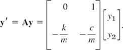
What kind of critical point does my″ + cy′ + ky = 0 in Sec. 2.4 have?
Solution. Division by m gives y″ = −(k/m)y − (c/m)y′. To get a system, set y1 = y, y2 = y′ (see Sec. 4.1). Then y′2 = y″ = −(k/m)y1 − (c/m)y2. Hence

We see that p = −c/m, q = k/m, Δ = (c/m)2 − 4k/m. From this and Tables 4.1 and 4.2 we obtain the following results. Note that in the last three cases the discriminant Δ plays an essential role.
No damping. c = 0, p = 0, q > 0, a center.
Underdamping. c2 < 4mk, p < 0, q > 0, Δ < 0, a stable and attractive spiral point.
Critical damping. c2 = 4mk, p < 0, q > 0, Δ = 0, a stable and attractive node.
Overdamping. c2 > 4mk, p < 0, q > 0, Δ > 0, a stable and attractive node.
1–10 TYPE AND STABILITY OF CRITICAL POINT
Determine the type and stability of the critical point. Then find a real general solution and sketch or graph some of the trajectories in the phase plane. Show the details of your work.
- y′1 = y1
y′2 = 2y2
- y′1 = −4y1
y′2 = −3y2
- y′1 = y2
y′2 = −9y1
- y′1 = 2y1 + y2
y′2 = 5y1 − 2y2
- y′1 = −2y1 + 2y2
y′2 = −2y1 − 2y2
- y′1 = −6y1 − y2
y′2 = −9y1 − 6y2
- y′1 = y1 + 2y2
y′2 = 2y1 + y2
- y′1 = −y1 + 4y2
y′2 = 3y1 − 2y2
- y′1 = 4y1 + y2
y′2 = 4y1 + 4y2
- y′1 = y2
y′2 = −5y1 − 2y2
11–18 TRAJECTORIES OF SYSTEMS AND SECOND-ORDER ODEs. CRITICAL POINTS
- 11. Damped oscillations. Solve y″ + 2y′ + 2y = 0. What kind of curves are the trajectories?
- 12. Harmonic oscillations. Solve
 . Find the trajectories. Sketch or graph some of them.
 - 13. Types of critical points. Discuss the critical points in (10)–(13) of Sec. 4.3 by using Tables 4.1 and 4.2.
- 14. Transformation of parameter. What happens to the critical point in Example 1 if you introduce τ = −t as a new independent variable?
- 15. Perturbation of center. What happens in Example 4 of Sec. 4.3 if you change A to A + 0.1I, where I is the unit matrix?
- 16. Perturbation of center. If a system has a center as its critical point, what happens if you replace the matrix A by
 with any real number k ≠ 0 (representing measurement errors in the diagonal entries)?
 - 17. Perturbation. The system in Example 4 in Sec. 4.3 has a center as its critical point. Replace each ajk in Example 4, Sec. 4.3, by ajk + b. Find values of b such that you get (a) a saddle point, (b) a stable and attractive node, (c) a stable and attractive spiral, (d) an unstable spiral, (e) an unstable node.
- 18. CAS EXPERIMENT. Phase Portraits. Graph phase portraits for the systems in Prob. 17 with the values of b suggested in the answer. Try to illustrate how the phase portrait changes “continuously” under a continuous change of b.
- 19. WRITING PROBLEM. Stability. Stability concepts are basic in physics and engineering. Write a two-part report of 3 pages each (A) on general applications in which stability plays a role (be as precise as you can), and (B) on material related to stability in this section. Use your own formulations and examples; do not copy.
- 20. Stability chart. Locate the critical points of the systems (10)–(14) in Sec. 4.3 and of Probs. 1, 3, 5 in this problem set on the stability chart.
4.5 Qualitative Methods for Nonlinear Systems
Qualitative methods are methods of obtaining qualitative information on solutions without actually solving a system. These methods are particularly valuable for systems whose solution by analytic methods is difficult or impossible. This is the case for many practically important nonlinear systems

In this section we extend phase plane methods, as just discussed, from linear systems to nonlinear systems (1). We assume that (1) is autonomous, that is, the independent variable t does not occur explicitly. (All examples in the last section are autonomous.) We shall again exhibit entire families of solutions. This is an advantage over numeric methods, which give only one (approximate) solution at a time.
Concepts needed from the last section are the phase plane (the y1y2-plane), trajectories (solution curves of (1) in the phase plane), the phase portrait of (1) (the totality of these trajectories), and critical points of (1) (points (y1, y2) at which both f1 (y1, y2) and f1(y1, y2) and f2(y1, y2 and zero).
Now (1) may have several critical points. Our approach shall be to discuss one critical point after another. If a critical point P0 is not at the origin, then, for technical convenience, we shall move this point to the origin before analyzing the point. More formally, if P0: (a, b) is a critical point with (a, b) not at the origin (0, 0), then we apply the translation
![]()
which moves P0 to (0, 0) as desired. Thus we can assume P0 to be the origin (0, 0), and for simplicity we continue to write y1, y2 (instead of ![]() ). We also assume that P0 is isolated, that is, it is the only critical point of (1) within a (sufficiently small) disk with center at the origin. If (1) has only finitely many critical points, that is automatically true. (Explain!)
). We also assume that P0 is isolated, that is, it is the only critical point of (1) within a (sufficiently small) disk with center at the origin. If (1) has only finitely many critical points, that is automatically true. (Explain!)
Linearization of Nonlinear Systems
How can we determine the kind and stability property of a critical point P0: (0, 0) of (1)? In most cases this can be done by linearization of (1) near P0, writing (1) as y′ = f(y) = Ay + h(y) and dropping h(y), as follows.
Since P0 is critical, f1(0, 0) = 0, f2(0, 0), so that f1 and f2 have no constant terms and we can write

A is constant (independent of t) since (1) is autonomous. One can prove the following (proof in Ref. [A7], pp. 375–388, listed in App. 1).
If f1 and f2 in (1) are continuous and have continuous partial derivatives in a neighborhood of the critical point P0: (0, 0), and if det A ≠ 0 in (2), then the kind and stability of the critical point of (1) are the same as those of the linearized system

Exceptions occur if A has equal or pure imaginary eigenvalues; then (1) may have the same kind of critical point as (3) or a spiral point.
EXAMPLE 1 Free Undamped Pendulum. Linearization
Figure 93a shows a pendulum consisting of a body of mass m (the bob) and a rod of length L. Determine the locations and types of the critical points. Assume that the mass of the rod and air resistance are negligible.
Solution. Step 1. Setting up the mathematical model. Let θ denote the angular displacement, measured counterclockwise from the equilibrium position. The weight of the bob is mg (g the acceleration of gravity). It causes a restoring force mg sin θ tangent to the curve of motion (circular arc) of the bob. By Newton's second law, at each instant this force is balanced by the force of acceleration mLθ″, where Lθ″ is the acceleration; hence the resultant of these two forces is zero, and we obtain as the mathematical model
![]()
Dividing this by mL, we have

When θ is very small, we can approximate sin θ rather accurately by θ and obtain as an approximate solution ![]() , but the exact solution for any θ is not an elementary function.
, but the exact solution for any θ is not an elementary function.
Step 2. Critical points (0, 0), (±2π, 0), (±4π, 0), …, Linearization. To obtain a system of ODEs, we set θ = y1, θ′ = y2. Then from (4) we obtain a nonlinear system (1) of the form

The right sides are both zero when y2 = 0 and sin y1 = 0. This gives infinitely many critical points (nπ, 0), where n = 0, ±1, ±2, …. We consider (0, 0). Since the Maclaurin series is
![]()
the linearized system at (0, 0) is
To apply our criteria in Sec. 4.4 we calculate p = a11 + a22 = 0, q = det A = k = g/L (>0), and Δ = p2 − 4q = −4k. From this and Table 4.1(c) in Sec. 4.4 we conclude that is a center, which is always stable. Since sin θ = sin y1 is periodic with period 2π, the critical points (nπ, 0), n = ±2, ±4, …, are all centers.
Step 3. Critical points (±π, 0), (±3π, 0), (±5π, 0), …, Linearization. We now consider the critical point (π, 0), setting θ − π = y1 and (θ − π)′ = θ′ = y2. Then in (4),
![]()
and the linearized system at (π, 0) is now
We see that p = 0, q = −k (<0), and Δ = −4q = 4k. Hence, by Table 4.1(b), this gives a saddle point, which is always unstable. Because of periodicity, the critical points (nπ, 0), n= ±1, ±3, …, are all saddle points. These results agree with the impression we get from Fig. 93b.

Fig. 93. Example 1 (C will be explained in Example 4.)
EXAMPLE 2 Linearization of the Damped Pendulum Equation
To gain further experience in investigating critical points, as another practically important case, let us see how Example 1 changes when we add a damping term cθ′ (damping proportional to the angular velocity) to equation (4), so that it becomes
![]()
where k > 0 and c ![]() 0 (which includes our previous case of no damping, c = 0). Setting θ = y1, θ′ = y2, as before, we obtain the nonlinear system (use θ″ = y′2)
0 (which includes our previous case of no damping, c = 0). Setting θ = y1, θ′ = y2, as before, we obtain the nonlinear system (use θ″ = y′2)
We see that the critical points have the same locations as before, namely, (0, 0), (±π, 0), (±2π, 0), …. We consider (0, 0). Linearizing sin y1 ≈ y2 as in Example 1, we get the linearized system at (0, 0)

This is identical with the system in Example 2 of Sec. 4.4, except for the (positive!) factor m (and except for the physical meaning of y1). Hence for c = 0 (no damping) we have a center (see Fig. 93b), for small damping we have a spiral point (see Fig. 94), and so on.
We now consider the critical point (π, 0). We set θ − π = y1, (θ − π)′ = θ′ = y2 and linearize
![]()
This gives the new linearized system at (π, 0)
For our criteria in Sec. 4.4 we calculate p = a11 + a22 = −c, q = det A = −k, and Δ = p2 − 4q = c2 + 4k. This gives the following results for the critical point at (π, 0).
No damping. c = 0, p = 0, q < 0, Δ > 0, a saddle point. See Fig. 93b.
Damping. c > 0, p < 0, q < 0, Δ > 0, a saddle point. See Fig. 94.
Since is periodic with period, 2π, the critical points (±2π, 0), (±4π, 0), … are of the same type as (0, 0), and the critical points (−π, 0), (±3π, 0), … are of the same type as (π, 0), so that our task is finished.
Figure 94 shows the trajectories in the case of damping. What we see agrees with our physical intuition. Indeed, damping means loss of energy. Hence instead of the closed trajectories of periodic solutions in Fig. 93b we now have trajectories spiraling around one of the critical points (0, 0), (±, 0), …. Even the wavy trajectories corresponding to whirly motions eventually spiral around one of these points. Furthermore, there are no more trajectories that connect critical points (as there were in the undamped case for the saddle points).
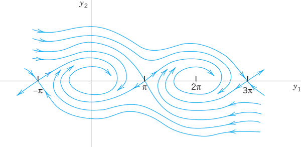
Fig. 94. Trajectories in the phase plane for the damped pendulum in Example 2
Lotka–Volterra Population Model
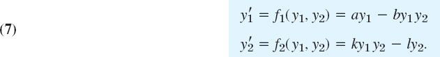
EXAMPLE 3 Predator–Prey Population Model3
This model concerns two species, say, rabbits and foxes, and the foxes prey on the rabbits.
Step 1. Setting up the model. We assume the following.
- Rabbits have unlimited food supply. Hence, if there were no foxes, their number y1(t) would grow exponentially, y′1 = ay1.
- Actually, y1 is decreased because of the kill by foxes, say, at a rate proportional to y1, y2, where y2(t) is the number of foxes. Hence y′1 = ay1 − by1y2, where a > 0 and b > 0.
- If there were no rabbits, then y2(t) would exponentially decrease to zero, y′2 = −ly2. However, y2 is increased by a rate proportional to the number of encounters between predator and prey; together we have y′2 = −ly2 + ky1y2, where k > 0 and l > 0.
This gives the (nonlinear!) Lotka–Volterra system
Step 2. Critical point (0, 0), Linearization. We see from (7) that the critical points are the solutions of
![]()
The solutions are (y1, y2) = (0, 0) and ![]() . We consider (0, 0). Dropping −by1y2 and ky1y2 from (7) gives the linearized system
. We consider (0, 0). Dropping −by1y2 and ky1y2 from (7) gives the linearized system

Its eigenvalues are λ1 = a > 0 and λ2 = −l < 0. They have opposite signs, so that we get a saddle point.
Step. 3. Critical point (l/k, a/b), Linearization. We set ![]() . Then the critical point (l/k, a/b) corresponds to
. Then the critical point (l/k, a/b) corresponds to ![]() . Since
. Since ![]() , we obtain from (7) [factorized as in (7*)]
, we obtain from (7) [factorized as in (7*)]
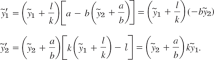
Dropping the two nonlinear terms ![]() and
and ![]() , we have the linearized system
, we have the linearized system
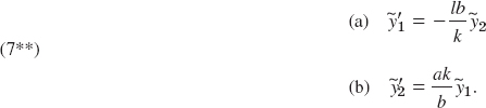
The left side of (a) times the right side of (b) must equal the right side of (a) times the left side of (b),
![]()
This is a family of ellipses, so that the critical point (l/k, a/b) of the linearized system (7**) is a center (Fig. 95). It can be shown, by a complicated analysis, that the nonlinear system (7) also has a center (rather than a spiral point) at (l/k, a/b) surrounded by closed trajectories (not ellipses).
We see that the predators and prey have a cyclic variation about the critical point. Let us move counterclockwise around the ellipse, beginning at the right vertex, where the rabbits have a maximum number. Foxes are sharply increasing in number until they reach a maximum at the upper vertex, and the number of rabbits is then sharply decreasing until it reaches a minimum at the left vertex, and so on. Cyclic variations of this kind have been observed in nature, for example, for lynx and snowshoe hare near the Hudson Bay, with a cycle of about 10 years.
For models of more complicated situations and a systematic discussion, see C. W. Clark, Mathematical Bioeconomics: The Mathematics of Conservation,3rd ed. Hoboken, NJ, Wiley, 2010.

Fig. 95. Ecological equilibrium point and trajectory of the linearized Lotka–Volterra system (7**)
Transformation to a First-Order Equation in the Phase Plane
Another phase plane method is based on the idea of transforming a second-order autonomous ODE (an ODE in which t does not occur explicitly)
![]()
to first order by taking y = y1 as the independent variable, setting y′ = y2 and transforming y′ by the chain rule,
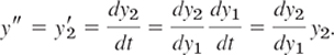
Then the ODE becomes of first order,
and can sometimes be solved or treated by direction fields. We illustrate this for the equation in Example 1 and shall gain much more insight into the behavior of solutions.
EXAMPLE 4 An ODE (8) for the Free Undamped Pendulum
If in (4)θ″ + k sin θ = 0 we set θ = y1, θ′ = y2 (the angular velocity) and use

Separation of variables gives y2dy2 = −k sin y1dy1. By integration,
![]()
Multiplying this by mL2, we get
![]()
We see that these three terms are energies. Indeed, y2 is the angular velocity, so that Ly2 is the velocity and the first term is the kinetic energy. The second term (including the minus sign) is the potential energy of the pendulum, and mL2C is its total energy, which is constant, as expected from the law of conservation of energy, because there is no damping (no loss of energy). The type of motion depends on the total energy, hence on C, as follows.
Figure 93b shows trajectories for various values of C. These graphs continue periodically with period 2π to the left and to the right. We see that some of them are ellipse-like and closed, others are wavy, and there are two trajectories (passing through the saddle points (nπ, 0), n = ±1, ±3, …) that separate those two types of trajectories. From (9) we see that the smallest possible C is C = −k; then y2 = 0, and cos y1 = 1, so that the pendulum is at rest. The pendulum will change its direction of motion if there are points at which y2 = θ′ = 0. Then k cos y1 + C = 0 by (9). If y1 = π, then cos y1 = −1 and C = k. Hence if −k < C < k, then the pendulum reverses its direction for a |y1| = |θ| < π, and for these values of C with |C| < k the pendulum oscillates. This corresponds to the closed trajectories in the figure. However, if C > k, then y2 = 0 is impossible and the pendulum makes a whirly motion that appears as a wavy trajectory in the y1y2-plane. Finally, the value C = k corresponds to the two “separating trajectories” in Fig. 93b connecting the saddle points.
The phase plane method of deriving a single first-order equation (8) may be of practical interest not only when (8) can be solved (as in Example 4) but also when a solution is not possible and we have to utilize fields (Sec. 1.2). We illustrate this with a very famous example:
EXAMPLE 5 Self-Sustained Oscillations. Van der Pol Equation
There are physical systems such that for small oscillations, energy is fed into the system, whereas for large oscillations, energy is taken from the system. In other words, large oscillations will be damped, whereas for small oscillations there is “negative damping” (feeding of energy into the system). For physical reasons we expect such a system to approach a periodic behavior, which will thus appear as a closed trajectory in the phase plane, called a limit cycle. A differential equation describing such vibrations is the famous van der Pol equation4
![]()
It first occurred in the study of electrical circuits containing vacuum tubes. For μ = 0 this equation becomes y″ + y = 0 and we obtain harmonic oscillations. Let μ > 0. The damping term has the factor −μ(1 − y2). This is negative for small oscillations, when y2 < 1, so that we have “negative damping,” is zero for y2 = 1 (no damping), and is positive if y2 > 1 (positive damping, loss of energy). If μ is small, we expect a limit cycle that is almost a circle because then our equation differs but little from y″ + y = 0. If ν is large, the limit cycle will probably look different.
Setting y = y1, y′ = y2 and using y″ = (dy2/dy1)y2 as in (8), we have from (10)

The isoclines in the y1y2-plane (the phase plane) are the curves dy2/dy1 = K = const, that is,
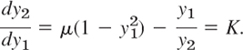
Solving algebraically for y2, we see that the isoclines are given by


Fig. 96. Direction field for the van der Pol equation with μ = 0.1 in the phase plane, showing also the limit cycle and two trajectories. See also Fig. 8 in Sec. 1.2
Figure 96 shows some isoclines when μ is small, μ = 0.1, the limit cycle (almost a circle), and two (blue) trajectories approaching it, one from the outside and the other from the inside, of which only the initial portion, a small spiral, is shown. Due to this approach by trajectories, a limit cycle differs conceptually from a closed curve (a trajectory) surrounding a center, which is not approached by trajectories. For larger μ the limit cycle no longer resembles a circle, and the trajectories approach it more rapidly than for smaller μ. Figure 97 illustrates this for μ = 1.
Fig. 97. Direction field for the van der Pol equation with μ = 1 in the phase plane, showing also the limit cycle and two trajectories approaching it
- Pendulum. To what state (position, speed, direction of motion) do the four points of intersection of a closed trajectory with the axes in Fig. 93b correspond? The point of intersection of a wavy curve with the y2-axis?
- Limit cycle. What is the essential difference between a limit cycle and a closed trajectory surrounding a center?
- CAS EXPERIMENT. Deformation of Limit Cycle. Convert the van der Pol equation to a system. Graph the limit cycle and some approaching trajectories for μ = 0.2, 0.4, 0.6, 0.8, 1.0, 1.5, 2.0. Try to observe how the limit cycle changes its form continuously if you vary μ continuously. Describe in words how the limit cycle is deformed with growing μ.
4–8 CRITICAL POINTS. LINEARIZATION
Find the location and type of all critical points by linearization. Show the details of your work.
- 4.

- 5.
- 6.

- 7.
- 8.

9–13 CRITICAL POINTS OF ODEs
Find the location and type of all critical points by first converting the ODE to a system and then linearizing it.
- 9. y″ − 9y + y3 = 0
- 10. y″ + y − y3 = 0
- 11. y″ + cos y = 0
- 12. y″ + 9y + y2 = 0
- 13. y″ + sin y = 0
- 14. TEAM PROJECT. Self-sustained oscillations. (a) Van der Pol equation. Determine the type of the critical point at (0, 0) when μ > 0, μ = 0, μ = < 0.
(b) Rayleigh equation. Show that the Rayleigh equation5

also describes self-sustained oscillations and that by differentiating it and setting y = Y′ one obtains the van der Pol equation.
(c) Duffing equation. The Duffing equation is
where usually |β| is small, thus characterizing a small deviation of the restoring force from linearity. β > 0 and β < 0 are called the cases of a hard spring and a soft spring, respectively. Find the equation of the trajectories in the phase plane. (Note that for β > 0 all these curves are closed.)
- 15. Trajectories. Write the ODE y″ − 4y + y3 = 0 as a system, solve it for y2 as a function of y1, and sketch or graph some of the trajectories in the phase plane.

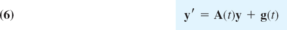
4.6 Nonhomogeneous Linear Systems of ODEs
In this section, the last one of Chap. 4, we discuss methods for solving nonhomogeneous linear systems of ODEs

where the vector g(t) is not identically zero. We assume g(t) and the entries of the n × n matrix A(t) to be continuous on some interval J of the t-axis. From a general solution y(h)(t) of the homogeneous system y′ = Ay on J and a particular solution y(p)(t) of (1) on J [i.e., a solution of (1) containing no arbitrary constants], we get a solution of (1),
y is called a general solution of (1) on J because it includes every solution of (1) on J. This follows from Theorem 2 in Sec. 4.2 (see Prob. 1 of this section).
Having studied homogeneous linear systems in Secs. 4.1–4.4, our present task will be to explain methods for obtaining particular solutions of (1). We discuss the method of undetermined coefficients and the method of the variation of parameters; these have counterparts for a single ODE, as we know from Secs. 2.7 and 2.10.
Method of Undetermined Coefficients
Just as for a single ODE, this method is suitable if the entries of A are constants and the components of g are constants, positive integer powers of t, exponential functions, or cosines and sines. In such a case a particular solution y(p) is assumed in a form similar to g; for instance, y(p) = u + vt + wt2 if g has components quadratic in t, with u, v, w to be determined by substitution into (1). This is similar to Sec. 2.7, except for the Modification Rule. It suffices to show this by an example.
EXAMPLE 1 Method of Undetermined Coefficients. Modification Rule
Find a general solution of
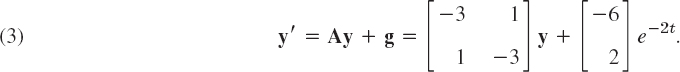
Solution. A general equation of the homogeneous system is (see Example 1 in Sec. 4.3)

Since λ = −2 is an eigenvalue of A, the function e−2t on the right side also appears in y(h), and we must apply the Modification Rule by setting
![]()
Note that the first of these two terms is the analog of the modification in Sec. 2.7, but it would not be sufficient here. (Try it.) By substitution,
![]()
Equating the te−2t-terms on both sides, we have −2u = Au. Hence u is an eigenvector of A corresponding to λ = −2; thus [see (5)] u = a[1 1]T with any a ≠ 0. Equating the other terms gives

Collecting terms and reshuffling gives
By addition, 0 = −2a − 4, a = −2, and then ν2 = ν1 + 4, say, ν1 = k, ν2 = k + 4, thus v = [k k + 4]T. We can simply choose k = 0. This gives the answer

For other k we get other v; for instance, k = −2 gives v = [−2 2]T, so that the answer becomes

Method of Variation of Parameters
This method can be applied to nonhomogeneous linear systems
with variable A = A(t) and general g(t). It yields a particular solution y(p) of (6) on some open interval J on the t- axis if a general solution of the homogeneous system y′ = A(t)y on J is known. We explain the method in terms of the previous example.
EXAMPLE 2 Solution by the Method of Variation of Parameters
Solve (3) in Example 1.
Solution. A basis of solutions of the homogeneous system is [e−2t e−2t]T and [e−4t −e−4t]T. Hence the general solution (4) of the homogeneous system may be written

Here, Y(t) = [y(1) y(2)] is the fundamental matrix (see Sec. 4.2). As in Sec. 2.10 we replace the constant vector c by a variable vector u(t) to obtain a particular solution
![]()
Substitution into (3) y′ = Ay + g gives
![]()
Now since y(1) and y(2) are solutions of the homogeneous system, we have
![]()
Hence Y′u = AYu, so that (8) reduces to
![]()
here we use that the inverse Y−1 of Y (Sec. 4.0) exists because the determinant of Y is the Wronskian W, which is not zero for a basis. Equation (9) in Sec. 4.0 gives the form of Y−1,
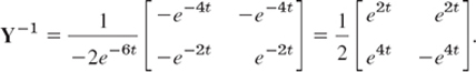
We multiply this by g, obtaining

Integration is done componentwise (just as differentiation) and gives

(where + 2 comes from the lower limit of integration). From this and Y in (7) we obtain

The last term on the right is a solution of the homogeneous system. Hence we can absorb it into y(h). We thus obtain as a general solution of the system (3), in agreement with (5*).

- Prove that (2) includes every solution of (1).
2–7 GENERAL SOLUTION
Find a general solution. Show the details of your work.
- 2. y′1 = y1 + y2 + 10 cos t
y′2 = 3y1 − y2 − 10 sin t
- 3. y′1 = y2 + e3t
y′2 = y1 − 3e3t
- 4. y′1 = 4y1 − 8y2 + 2 cosh t
y′2 = 2y1 − 6y2 + cosh t + 2 sinh t
- 5. y′1 = 4y1 + y2 + 0.6t
y′2 = 2y1 + 3y2 − 2.5t
- 6. y′1 = 4y2
y′2 = 4y1 − 16t2 + 2
- 7. y′1 = −3y1 − 4y2 + 11t + 15
y′2 = 5y1 + 6y2 + 3e−t − 15t − 20
- 8. CAS EXPERIMENT. Undetermined Coefficients. Find out experimentally how general you must choose y(p), in particular when the components of g have a different form (e.g., as in Prob. 7). Write a short report, covering also the situation in the case of the modification rule.
- 9. Undetermined Coefficients. Explain why, in Example 1 of the text, we have some freedom in choosing the vector v.
10–15 INITIAL VALUE PROBLEM
Solve, showing details:
- 10.
- 11.

- 12.

- 13.

- 14.

- 15.

- 16. WRITING PROJECT. Undetermined Coefficients. Write a short report in which you compare the application of the method of undetermined coefficients to a single ODE and to a system of ODEs, using ODEs and systems of your choice.
17–20 NETWORK
Find the currents in Fig. 99 (Probs. 17–19) and Fig. 100 (Prob. 20) for the following data, showing the details of your work.
- 17. R1 = 2 Ω, R2 = 8 Ω, L = 1 H, C = 0.5 F, E = 200 V
- 18. Solve Prob. 17 with E = 440 sin t V and the other data as before.
- 19. In Prob. 17 find the particular solution when currents and charge at t = 0 are zero.
- 20. R1 = 1 Ω, R2 = 1.4 Ω, L1 = 0.8 H, L2 = 1 H, E = 100 V, I1(0) = I2(0) = 0

CHAPTER 4 REVIEW QUESTIONS AND PROBLEMS
- State some applications that can be modeled by systems of ODEs.
- What is population dynamics? Give examples.
- How can you transform an ODE into a system of ODEs?
- What are qualitative methods for systems? Why are they important?
- What is the phase plane? The phase plane method? A trajectory? The phase portrait of a system of ODEs?
- What are critical points of a system of ODEs? How did we classify them? Why are they important?
- What are eigenvalues? What role did they play in this chapter?
- What does stability mean in general? In connection with critical points? Why is stability important in engineering?
- What does linearization of a system mean?
- Review the pendulum equations and their linearizations.
11–17 GENERAL SOLUTION. CRITICAL POINTS
Find a general solution. Determine the kind and stability of the critical point.
- 11. y′1 = 2y2
y′2 = 8y1
- 12. y′1 = 5y1
y′2 = y2
- 13. y′1 = −2y1 + 5y2
y′2 = −y1 − 6y2
- 14. y′1 = 3y1 + 4y2
y′2 = 3y1 + 2y2
- 15. y′1 = −3y1 − 2y2
y′2 = −2y1 − 3y2
- 16. y′1 = 4y2
y′2 = − 4y1
- 17. y′1 = −y1 + 2y2
y′2 = −2y1 − y2
18–19 CRITICAL POINT
What kind of critical point does y′ = Ay have if A has the eigenvalues
- 18. −4 and 2
- 19. 2 + 3i, 2 − 3i
20–23 NONHOMOGENEOUS SYSTEMS
Find a general solution. Show the details of your work.
- 20. y′1 = 2y1 + 2y2 + et
y′2 = −2y1 − 3y2 + et
- 21. y′1 = 4y2
y′2 = 4y1 + 32t2
- 22. y′1 = y1 + y2 + sin t
y′2 = 4y1 + y2
- 23. y′1 = y1 + 4y2 − 2 cos t
y′2 = y1 + y2 − cos t + sin t
- 24. Mixing problem. Tank T1 in Fig. 101 initially contains 200 gal of water in which 160 lb of salt are dissolved. Tank T2 initially contains 100 gal of pure water. Liquid is pumped through the system as indicated, and the mixtures are kept uniform by stirring. Find the amounts of salt y1(t) and y2(t) in T1 and T2, respectively.
- 25. Network. Find the currents in Fig. 102 when R = 2.5 Ω, L = 1 H, C = 0.04 F, E(t) = 169 sin t V, I1(0) = 0, I2(0) = 0.
- 26. Network. Find the currents in Fig. 103 when R = 1 Ω, L = 1.25 H, C = 0.2 F, I1(0) = 1 A, I2(0) = 1 A.
20–23 LINEARIZATION
Find the location and kind of all critical points of the given nonlinear system by linearization.
- 27.

- 28. y′1 = cos y2
y′2 = 3y1
- 29. y′1 = −4y2
y′2 = sin y1
- 30.

SUMMARY OF CHAPTER 4 Systems of ODEs. Phase Plane. Qualitative Methods
Whereas single electric circuits or single mass–spring systems are modeled by single ODEs (Chap. 2), networks of several circuits, systems of several masses and springs, and other engineering problems lead to systems of ODEs, involving several unknown functions y1(t), …, yn(t). Of central interest are first-order systems (Sec. 4.2):

to which higher order ODEs and systems of ODEs can be reduced (Sec. 4.1). In this summary we let n = 2, so that

Then we can represent solution curves as trajectories in the phase plane (the y1y2-plane), investigate their totality [the “phase portrait” of (1)], and study the kind and stability of the critical points (points at which both f1 and f2 are zero), and classify them as nodes, saddle points, centers, orspiral points (Secs. 4.3, 4.4). These phase plane methods are qualitative; with their use we can discover various general properties of solutions without actually solving the system. They are primarily used for autonomous systems, that is, systems in which t does not occur explicitly.
A linear system is of the form

If g = 0, the system is called homogeneous and is of the form
![]()
If a11, …, a22 are constants, it has solutions y = xeλt, where λ is a solution of the quadratic equation

and x ≠ 0 has components x1, x2 determined up to a multiplicative constant by
![]()
(These λ's are called the eigenvalues and these vectors x eigenvectors of the matrix A. Further explanation is given in Sec. 4.0.)
A system (2) with g ≠ 0 is called nonhomogeneous. Its general solution is of the form y = yh + yp, where yh is a general solution of (3) and yp a particular solution of (2). Methods of determining the latter are discussed in Sec. 4.6.
The discussion of critical points of linear systems based on eigenvalues is summarized in Tables 4.1 and 4.2 in Sec. 4.4. It also applies to nonlinear systems if the latter are first linearized. The key theorem for this is Theorem 1 in Sec. 4.5, which also includes three famous applications, namely the pendulum and van der Pol equations and the Lotka–Volterra predator–prey population model.
1A name that comes from physics, where it is the y-(mv)-plane, used to plot a motion in terms of position y and velocity y′ = v (m = mass); but the name is now used quite generally for the y1y2-plane.
The use of the phase plane is a qualitative method, a method of obtaining general qualitative information on solutions without actually solving an ODE or a system. This method was created by HENRI POINCARÉ (1854–1912), a great French mathematician, whose work was also fundamental in complex analysis, divergent series, topology, and astronomy.
2In the sense of the Russian mathematician ALEXANDER MICHAILOVICH LJAPUNOV (1857–1918), whose work was fundamental in stability theory for ODEs. This is perhaps the most appropriate definition of stability (and the only we shall use), but there are others, too.
3Introduced by ALFRED J. LOTKA (1880–1949), American biophysicist, and VITO VOLTERRA (1860–1940), Italian mathematician, the initiator of functional analysis (see [GR7] in App. 1).
4BALTHASAR VAN DER POL (1889–1959), Dutch physicist and engineer.
5LORD RAYLEIGH (JOHN WILLIAM STRUTT) (1842–1919), English physicist and mathematician, professor at Cambridge and London, known by his important contributions to the theory of waves, elasticity theory, hydrodynamics, and various other branches of applied mathematics and theoretical physics. In 1904 he was awarded the Nobel Prize in physics.