
CHAPTER 24
Data Analysis.
Probability Theory

We first show how to handle data numerically or in terms of graphs, and how to extract information (average size, spread of data, etc.) from them. If these data are influenced by “chance,” by factors whose effect we cannot predict exactly (e.g., weather data, stock prices, life spans of tires, etc.), we have to rely on probability theory. This theory originated in games of chance, such as flipping coins, rolling dice, or playing cards. Nowadays it gives mathematical models of chance processes called random experiments or, briefly, experiments. In such an experiment we observe a random variable X, that is, a function whose values in a trial (a performance of an experiment) occur “by chance” (Sec. 24.3) according to a probability distribution that gives the individual probabilities with which possible values of X may occur in the long run. (Example: Each of the six faces of a die should occur with the same probability, 1/6.) Or we may simultaneously observe more than one random variable, for instance, height and weight of persons or hardness and tensile strength of steel. This is discussed in Sec. 24.9, which will also give the basis for the mathematical justification of the statistical methods in Chapter 25.
Prerequisite: Calculus.
References and Answers to Problems: App. 1 Part G, App. 2.
24.1 Data Representation. Average. Spread
Data can be represented numerically or graphically in various ways. For instance, your daily newspaper may contain tables of stock prices and money exchange rates, curves or bar charts illustrating economical or political developments, or pie charts showing how your tax dollar is spent. And there are numerous other representations of data for special purposes.
In this section we discuss the use of standard representations of data in statistics. (For these, software packages, such as DATA DESK, R, and MINITAB, are available, and Maple or Mathematica may also be helpful; see pp. 789 and 1009) We explain corresponding concepts and methods in terms of typical examples.
EXAMPLE 1 Recording and Sorting
Sample values (observations, measurements) should be recorded in the order in which they occur. Sorting, that is, ordering the sample values by size, is done as a first step of investigating properties of the sample and graphing it. Sorting is a standard process on the computer; see Ref. [E35], listed in App. 1.
Super alloys is a collective name for alloys used in jet engines and rocket motors, requiring high temperature (typically 1800°F), high strength, and excellent resistance to oxidation. Thirty specimens of Hastelloy C (nickel-based steel, investment cast) had the tensile strength (in 1000 lb/sq in.), recorded in the order obtained and rounded to integer values,

Sorting gives

Graphic Representation of Data
We shall now discuss standard graphic representations used in statistics for obtaining information on properties of data.
EXAMPLE 2 Stem-and-Leaf Plot (Fig. 507)
This is one of the simplest but most useful representations of data. For (1) it is shown in Fig. 507. The numbers in (1) range from 78 to 99; see (2). We divide these numbers into 5 groups, 75–79, 80–84, 85–89, 90–94, 95–99. The integers in the tens position of the groups are 7, 8, 8, 9, 9. These form the stem in Fig. 507. The first leaf is 789, representing 77, 78, 79. The second leaf is 1123344, representing 81, 81, 82, 83, 83, 84, 84. And so on.
The number of times a value occurs is called its absolute frequency. Thus 78 has absolute frequency 1, the value 89 has absolute frequency 5, etc. The column to the extreme left in Fig. 507 shows the cumulative absolute frequencies, that is, the sum of the absolute frequencies of the values up to the line of the leaf. Thus, the number 10 in the second line on the left shows that (1) has 10 values up to and including 84. The number 23 in the next line shows that there are 23 values not exceeding 89, etc. Dividing the cumulative absolute frequencies by n(= 30 in Fig. 507) gives the cumulative relative frequencies0.1, 0.33, 0.76, 0.93, 1.00.
EXAMPLE 3 Histogram (Fig. 508)
For large sets of data, histograms are better in displaying the distribution of data than stem-and-leaf plots. The principle is explained in Fig. 508. (An application to a larger data set is shown in Sec. 25.7). The bases of the rectangles in Fig. 508 are the x-intervals (known as class intervals) 74.5–79.5, 79.5–84.5, 84.5–89.5, 89.5–94.5, 94.5–99.5, whose midpoints (known as class marks) are x = 77, 82, 87, 92, 97, respectively. The height of a rectangle with class mark x is the relative class frequency frel(x), defined as the number of data values in that class interval, divided by n (= 30 in our case). Hence the areas of the rectangles are proportional to these relative frequencies, 0.10, 0.23, 0.43, 0.17, 0.07, so that histograms give a good impression of the distribution of data.

Fig. 507. Stem-and-leaf plot of the data in Example 1
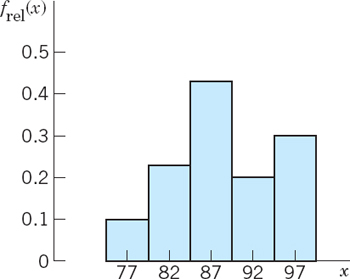
Fig. 508. Histogram of the data in Example 1 (grouped as in Fig. 507)
EXAMPLE 4 Boxplot. Median. Interquartile Range. Outlier
A boxplot of a set of data illustrates the average size and the spread of the values, in many cases the two most important quantities characterizing the set, as follows.
The average size is measured by the median, or middle quartile, qM. If the number n of values of the set is odd, then qM is the middlemost of the values when ordered as in (2). If n is even, then qM is the average of the two middlemost values of the ordered set. In (2) we have n = 30 and thus ![]() . (In general, will be a fraction if n is even.)
. (In general, will be a fraction if n is even.)
The spread of values can be measured by the range R = xmax − xmin, the largest value minus the smallest one.
Better information on the spread gives the interquartile range IQR = qU − qL. Here qU is the middlemost value (or the average of the two middlemost values) in the data above the median; and qL is the middlemost value (or the average of the two middlemost values) in the data below the median. Hence in (2) we have qU = x23 = 89, qL = x8 = 83, and IQR = 89 − 83 = 6.
The box in Fig. 509 extends vertically from qL to qU; it has height IQR = 6. The vertical lines below and above the box extend from xmin = 77 to xmax = 99, so that they show R = 22.
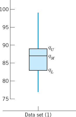
Fig. 509. Boxplot of the data set (1)
The line above the box is suspiciously long. This suggests the concept of an outlier, a value that is more than 1.5 times the IQR away from either end of the box; here 1.5 is purely conventional. An outlier indicates that something might have gone wrong in the data collection. In (2) we have 89 + 1.5 IQR = 98, and we regard 99 as an outlier.
Mean. Standard Deviation. Variance.
Empirical Rule
Medians and quartiles are easily obtained by ordering and counting, practically without calculation. But they do not give full information on data: you can change data values to some extent without changing the median. Similarly for the quartiles.
The average size of the data values can be measured in a more refined way by the mean
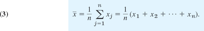
This is the arithmetic mean of the data values, obtained by taking their sum and dividing by the data size n. Thus in (1),
![]()
Every data value contributes, and changing one of them will change the mean.
Similarly, the spread (variability) of the data values can be measured in a more refined way by the standard deviation s or by its square, the variance
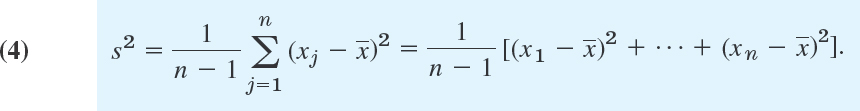
Thus, to obtain the variance of the data, take the difference ![]() of each data value from the mean, square it, take the sum of these n squares, and divide it by n − 1 (not n, as we motivate in Sec. 25.2). To get the standard deviation s, take the square root of s2.
of each data value from the mean, square it, take the sum of these n squares, and divide it by n − 1 (not n, as we motivate in Sec. 25.2). To get the standard deviation s, take the square root of s2.
For example, using ![]() , we get for the data (1) the variance
, we get for the data (1) the variance
![]()
Hence the standard deviation is ![]() . Note that the standard deviation has the same dimension as the data values (kg/mm2, see at the beginning), which is an advantage. On the other hand, the variance is preferable to the standard deviation in developing statistical methods, as we shall see in Chap. 25.
. Note that the standard deviation has the same dimension as the data values (kg/mm2, see at the beginning), which is an advantage. On the other hand, the variance is preferable to the standard deviation in developing statistical methods, as we shall see in Chap. 25.
CAUTION! Your CAS (Maple, for instance) may use 1/n instead of 1/(n − 1) in (4), but the latter is better when n is small (see Sec. 25.2).
Mean and standard deviation, introduced to give center and spread, actually give much more information according to this rule.
Empirical Rule. For any mound-shaped, nearly symmetric distribution of data the intervals
![]()
respectively, of the data points.
EXAMPLE 5 Empirical Rule and Outliers. z-Score
For (1), with ![]() and s = 4.8, the three intervals in the Rule are 81.9
and s = 4.8, the three intervals in the Rule are 81.9 ![]() x
x ![]() 91.5, 77.1
91.5, 77.1 ![]() x
x ![]() 96.3, 72.3
96.3, 72.3 ![]() x
x ![]() 101.1 and contain 73% (22 values remain, 5 are too small, and 5 too large), 93% (28 values, 1 too small, and 1 too large), and 100%, respectively.
101.1 and contain 73% (22 values remain, 5 are too small, and 5 too large), 93% (28 values, 1 too small, and 1 too large), and 100%, respectively.
If we reduce the sample by omitting the outlier 99, mean and standard deviation reduce to ![]() , approximately, and the percentage values become 67% (5 and 5 values outside), 93% (1 and 1 outside), and 100%
, approximately, and the percentage values become 67% (5 and 5 values outside), 93% (1 and 1 outside), and 100%
Finally, the relative position of a value x in a set of mean ![]() and standard deviation s can be measured by the z-score
and standard deviation s can be measured by the z-score
![]()
This is the distance of x from the mean ![]() measured in multiples of s. For instance, z(83) = (83 − 86.7)/4.8 = −0.77. This is negative because 83 lies below the mean. By the Empirical Rule, the extreme z-values are about −3 and 3.
measured in multiples of s. For instance, z(83) = (83 − 86.7)/4.8 = −0.77. This is negative because 83 lies below the mean. By the Empirical Rule, the extreme z-values are about −3 and 3.
1–10 DATA REPRESENTATIONS
Represent the data by a stem-and-leaf plot, a histogram, and a boxplot:
- Length of nails [mm]

- Phone calls per minute in an office between 9.00 A.M. and A.M.

- Systolic blood pressure of 15 female patients of ages 20–22

- Iron content [%] of 15 specimens of hermatite (Fe2O3)

- Weight of filled bags [g] in an automatic filling

- Gasoline consumption [miles per gallon, rounded] of six cars of the same model under similar conditions

- Release time [sec] of a relay

- Foundrax test of Brinell hardness (2.5 mm steel ball, 62.5 kg load, 30 sec) of 20 copper plates (values in kg/mm2)

- Efficiency [%] of seven Voith Francis turbines of runner diameter 2.3 m under a head range of 185 m

- −0.51 0.12 −0.47 0.95 0.25 −0.18 −0.54
11–16 AVERAGE AND SPREAD
Find the mean and compare it with the median. Find the standard deviation and compare it with the interquartile range.
- 11. For the data in Prob. 1
- 12. For the phone call data in Prob. 2
- 13. For the medical data in Prob. 3
- 14. For the iron contents in Prob. 4
- 15. For the release times in Prob. 7
- 16. For the Brinell hardness data in Prob. 8
- 17. Outlier, reduced data. Calculate s for the data 4 1 3 10 2. Then reduce the data by deleting the outlier and calculate s. Comment.
- 18. Outlier, reduction. Do the same tasks as in Prob. 17 for the hardness data in Prob. 8.
- 19. Construct the simplest possible data with
 but qM = 0. What is the point of this problem?
 - 20. Mean. Prove that
 must always lie between the smallest and the largest data values.
24.2 Experiments, Outcomes, Events
We now turn to probability theory. This theory has the purpose of providing mathematical models of situations affected or even governed by “chance effects,” for instance, in weather forecasting, life insurance, quality of technical products (computers, batteries, steel sheets, etc.), traffic problems, and, of course, games of chance with cards or dice. And the accuracy of these models can be tested by suitable observations or experiments—this is a main purpose of statistics to be explained in Chap. 25.
We begin by defining some standard terms. An experiment is a process of measurement or observation, in a laboratory, in a factory, on the street, in nature, or wherever; so “experiment” is used in a rather general sense. Our interest is in experiments that involve randomness, chance effects, so that we cannot predict a result exactly. A trial is a single performance of an experiment. Its result is called an outcome or a sample point. n trials then give a sample of size n consisting of n sample points. The sample space S of an experiment is the set of all possible outcomes.
EXAMPLES 1–6 Random Experiments. Sample Spaces
- Inspecting a lightbulb. S = {Defective, Nondefective}.
- Rolling a die. S = {1, 2, 3, 4, 5, 6}.
- Measuring tensile strength of wire. S the numbers in some interval.
- Measuring copper content of brass. s: 50% to 90%, say.
- Counting daily traffic accidents in New York. S the integers in some interval.
- Asking for opinion about a new car model. S = {Like, Dislike, Undecided}.
The subsets of S are called events and the outcomes simple events.
In (2), events are A = {1, 3, 5} (“Odd number”), B = {2, 4, 6} (“Even number”), C = {5, 6}. etc. Simple events are {1}, {2}, …, {6}.
If, in a trial, an outcome a happens and a ∈ A (a is an element of A), we say that A happens. For instance, if a die turns up a 3, the event A: Odd number happens. Similarly, if C in Example 7 happens (meaning 5 or 6 turns up), then, say, D = {4, 5, 6} happens. Also note that S happens in each trial, meaning that some event of S always happens. All this is quite natural.
Unions, Intersections, Complements of Events
In connection with basic probability laws we shall need the following concepts and facts about events (subsets) A, B, C, … of a given sample space S.
The union A ∪ B of A and B consists of all points in A or B or both.
The intersection A ∩ B of A and B consists of all points that are in both A and B.
If A and B have no points in common, we write
![]()
where Ø is the empty set (set with no elements) and we call A and B mutually exclusive (or disjoint) because, in a trial, the occurrence of A excludes that of B (and conversely)—if your die turns up an odd number, it cannot turn up an even number in the same trial. Similarly, a coin cannot turn up Head and Tail at the same time.
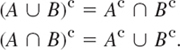
Complement Ac of A. This is the set of all the points of S not in A. Thus,
![]()
In Example 7 we have Ac = B, hence A ∪ Ac = {1, 2, 3, 4, 5, 6} = S.
Another notation for the complement of A is ![]() (instead of Ac), but we shall not use this because in set theory
(instead of Ac), but we shall not use this because in set theory ![]() is used to denote the closure of A (not needed in our work).
is used to denote the closure of A (not needed in our work).
Unions and intersections of more events are defined similarly. The union
![]()
of events A1, …, Am consists of all points that are in at least one Aj. Similarly for the union A1 ∪ A2 ∪ … of infinitely many subsets A1, A2, … of an infinite sample space S (that is, S consists of infinitely many points). The intersection
![]()
of A1, …, Am consists of the points of S that are in each of these events. Similarly for the intersection A1 ∩ A2 ∩ … of infinitely many subsets of S.
Working with events can be illustrated and facilitated by Venn diagrams1 for showing unions, intersections, and complements, as in Figs. 510 and 511, which are typical examples that give the idea.
EXAMPLE 8 Unions and Intersections of 3 Events
In rolling a die, consider the events
![]()
Then A ∩ B = {4, 5}, B ∩ C = {2, 4}, C ∩ A = {4, 6}, A ∩ B ∩ C = {4}. Can you sketch a Venn diagram of this? Furthermore, A ∪ B = s, hence A ∪ B = s, hence A ∪ B ∪ C = s (why?).

Fig. 510. Venn diagrams showing two events A and B in a sample space S and their union A ∪ B (colored) and intersection A ∩ B (colored)
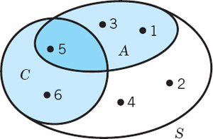
Fig. 511. Venn diagram for the experiment of rolling a die, showing S, A = {1, 3, 5}, C = {5, 6}, A ∪ C = {1, 3, 5, 6}, A ∩ C = {5}
1–12 SAMPLE SPACES, EVENTS
Graph a sample space for the experiments:
- Drawing 3 screws from a lot of right-handed and left-handed screws
- Tossing 2 coins
- Rolling 2 dice
- Rolling a die until the first Six appears
- Tossing a coin until the first Head appears
- Recording the lifetime of each of 3 lightbulbs
- Recording the daily maximum temperature X and the daily maximum air pressure Y at Times Square in New York
- Choosing a committee of 2 from a group of 5 people
- Drawing gaskets from a lot of 10, containing one defective D, unitil D is drawn, one at a time and assuming sampling without replacement, that is, gaskets drawn are not returned to the lot. (More about this in Sec. 24.6)
- In rolling 3 dice, are the events A: Sum divisible by 3 and B: Sum divisible by 5 mutually exclusive?
- Answer the questions in Prob. 10 for rolling 2 dice.
- List all 8 subsets of the sample space S = {a, b, c}.
- In Prob. 3 circle and mark the events A: Faces are equal, B: Sum of faces less than 5, A ∪ B, A ∩ B, Ac, Bc.
- In drawing 2 screws from a lot of right-handed and left-handed screws, let A, B, C, D mean at a least 1 right-handed, at least 1 left-handed, 2 right-handed, 2 left-handed, respectively. Are A and B mutually exclusive? C and D?
15–20 VENN DIAGRAMS
- 15. In connection with a trip to Europe by some students, consider the events P that they see Paris, G that they have a good time, and M that they run out of money, and describe in words the events 1, …, 7 in the diagram.

Problem 15
- 16. Show that, by the definition of complement, for any subset A of a sample space S.

- 17. Using a Venn diagram, show that A ⊆ B if and only if A ∪ B = B.
- 18. Using a Venn diagram, show that A ⊆ B if and only if A ∩ B = A.
- 19. (De Morgan's laws) Using Venn diagrams, graph and check De Morgan's laws
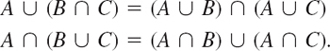
- 20. Using Venn diagrams, graph and check the rules
24.3 Probability
The “probability” of an event A in an experiment is supposed to measure how frequently A is about to occur if we make many trials. If we flip a coin, then heads H and tails T will appear about equally often—we say that H and T are “equally likely.” Similarly, for a regularly shaped die of homogeneous material (“fair die”) each of the six outcomes 1, …, 6 will be equally likely. These are examples of experiments in which the sample space S consists of finitely many outcomes (points) that for reasons of some symmetry can be regarded as equally likely. This suggests the following definition.
DEFINITION 1 First Definition of Probability
If the sample space S of an experiment consists of finitely many outcomes (points) that are equally likely, then the probability P(A) of an event A is
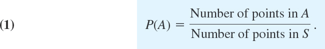
From this definition it follows immediately that, in particular,

In rolling a fair die once, what is the probability P(A) of A of obtaining a 5 or a 6? The probability of B:“Even number”?
Solution. The six outcomes are equally likely, so that each has probability 1/6. Thus P(A) = 2/6 = 1/3 because A = {5, 6} has 2 points, and P(B) = 3/6 = 1/2.
Definition 1 takes care of many games as well as some practical applications, as we shall see, but certainly not of all experiments, simply because in many problems we do not have finitely many equally likely outcomes. To arrive at a more general definition of probability, we regard probability as the counterpart of relative frequency. Recall from Sec. 24.1 that the absolute frequency f(A) of an event A in n trials is the number of times A occurs, and the relative frequency of A in these trials is f(A)/n; thus

Now if A did not occur, then f(A) = 0. If A always occurred, then f(A) = n. These are the extreme cases. Division by n gives
![]()
In particular, for A = S we have f(S) = n because S always occurs (meaning that some event always occurs; if necessary, see Sec. 24.2, after Example 7). Division by n gives
![]()
Finally, if A and B are mutually exclusive, they cannot occur together. Hence the absolute frequency of their union A ∪ B must equal the sum of the absolute frequencies of A and B. Division by n gives the same relation for the relative frequencies,
![]()
We are now ready to extend the definition of probability to experiments in which equally likely outcomes are not available. Of course, the extended definition should include Definition 1. Since probabilities are supposed to be the theoretical counterpart of relative frequencies, we choose the properties in (4*), (5*), (6*) as axioms. (Historically, such a choice is the result of a long process of gaining experience on what might be best and most practical.)
DEFINITION 2 General Definition of Probability
Given a sample space S, with each event A of S (subset of S) there is associated a number P(A), called the probability of A, such that the following axioms of probability are satisfied.
1. For every A in S,
2. The entire sample space S has the probability

3. For mutually exclusive events A and B (A ∩ B) = Ø; see Sec. 24.2),

If S is infinite (has infinitely many points), Axiom 3 has to be replaced by 3′. For mutually exclusive events A1, A2, …,
![]()
In the infinite case the subsets of S on which P(A) is defined are restricted to form a so-called σ-algebra, as explained in Ref. [GenRef6] (not [G6]!) in App. 1. This is of no practical consequence to us.
Basic Theorems of Probability
We shall see that the axioms of probability will enable us to build up probability theory and its application to statistics. We begin with three basic theorems. The first of them is useful if we can get the probability of the complement Ac more easily than P(A) itself.
PROOF
By the definition of complement (Sec. 24.2), we have S = A ∪ Ac and A ∩ Ac = Ø. Hence by Axioms 2 and 3,
![]()
Five coins are tossed simultaneously. Find the probability of the event A: At least one head turns up. Assume that the coins are fair.
Solution. Since each coin can turn up heads or tails, the sample space consists of 25 = 32 outcomes. Since the coins are fair, we may assign the same probability (1/32) to each outcome. Then the event Ac (No heads turn up) consists of only 1 outcome. Hence P(Ac) = 1/32, and the answer is P(A) = 1 − P(Ac) = 31/32.
The next theorem is a simple extension of Axiom 3, which you can readily prove by induction.
THEOREM 2 Addition Rule for Mutually Exclusive Events
For mutually exclusive events A1, …, Am in a sample space S,
![]()
EXAMPLE 3 Mutually Exclusive Events
If the probability that on any workday a garage will get 10–20, 21–30, 31–40, over 40 cars to service is 0.20, 0.35, 0.25, 0.12, respectively, what is the probability that on a given workday the garage gets at least 21 cars to service?
Solution. Since these are mutually exclusive events, Theorem 2 gives the answer 0.35 + 0.25 + 0.12 = 0.72. Check this by the complementation rule.
In many cases, events will not be mutually exclusive. Then we have

PROOF
C, D, E in Fig. 512 make up A ∪ B and are mutually exclusive (disjoint). Hence by Theorem 2,
![]()
This gives (9) because on the right P(C) + P(D) = P(A) by Axiom 3 and disjointness; and P(E) = P(B) − P(D) = P(B) − P(A ∩ B), also by Axiom 3 and disjointness.

Fig. 512. Proof of Theorem 3
Note that for mutually exclusive events A and B we have A ∩ B = Ø by definition and, by comparing (9) and (6),
(Can you also prove this by (5) and (7)?)
EXAMPLE 4 Union of Arbitrary Events
In tossing a fair die, what is the probability of getting an odd number or a number less than 4?
Solution. Let A be the event “Odd number” and B the event “Number less than 4.” Then Theorem 3 gives the answer
![]()
because A ∩ B = “Odd number less than 4” = {1, 3}.
Conditional Probability. Independent Events
Often it is required to find the probability of an event B under the condition that an event A occurs. This probability is called the conditional probability of B given A and is denoted by P(B|A). In this case A serves as a new (reduced) sample space, and that probability is the fraction of P(A) which corresponds to A ∩ B. Thus

Similarly, the conditional probability of A given B is

Solving (11) and (12) for P (A ∩ B) we obtain
If A and B are events in a sample space S and P(A) ≠ 0, P(B) ≠ 0, then

In producing screws, let A mean “screw too slim” and B “screw too short.” Let P(A) = 0.1 and let the conditional probability that a slim screw is also too short be P(B|A) = 0.2. What is the probability that a screw that we pick randomly from the lot produced will be both too slim and too short?
Solution. P(A ∩ B) = P(A)P(B|A) = 0.1 · 0.2 = 0.02 = 2%, by Theorem 4.
Independent Events. If events A and B are such that

they are called independent events. Assuming P(A) ≠ 0, P(B) ≠ 0, we see from (11)–(13) that in this case
![]()
This means that the probability of A does not depend on the occurrence or nonoccurrence of B, and conversely. This justifies the term “independent.”
Independence of m Events. Similarly, m events A1, …, Am are called independent if
![]()
as well as for every k different events Aj1, Aj2, …, Ajk.
![]()
where k = 2, 3, …, m − 1.
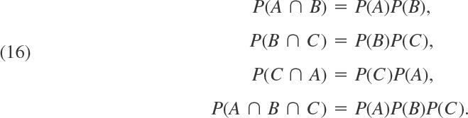
Accordingly, three events A, B, C are independent if and only if
Sampling. Our next example has to do with randomly drawing objects, one at a time, from a given set of objects. This is called sampling from a population, and there are two ways of sampling, as follows.
- In sampling with replacement, the object that was drawn at random is placed back to the given set and the set is mixed thoroughly. Then we draw the next object at random.
- In sampling without replacement the object that was drawn is put aside.
EXAMPLE 6 Sampling With and Without Replacement
A box contains 10 screws, three of which are defective. Two screws are drawn at random. Find the probability that neither of the two screws is defective.
Solution. We consider the events

Clearly, ![]() because 7 of the 10 screws are nondefective and we sample at random, so that each screw has the same probability
because 7 of the 10 screws are nondefective and we sample at random, so that each screw has the same probability ![]() of being picked. If we sample with replacement, the situation before the second drawing is the same as at the beginning, and
of being picked. If we sample with replacement, the situation before the second drawing is the same as at the beginning, and ![]() . The events are independent, and the answer is
. The events are independent, and the answer is
![]()
If we sample without replacement, then ![]() , as before. If A has occurred, then there are 9 screws left in the box, 3 of which are defective. Thus
, as before. If A has occurred, then there are 9 screws left in the box, 3 of which are defective. Thus ![]() , and Theorem 4 yields the answer
, and Theorem 4 yields the answer
![]()
Is it intuitively clear that this value must be smaller than the preceding one?
- In rolling 3 fair dice, what is the probability of obtaining a sum not greater than 16?
- In rolling 2 fair dice, what is the probability of a sum greater than 3 but not exceeding 6?
- Three screws are drawn at random from a lot of 100 screws, 10 of which are defective. Find the probability of the event that all 3 screws drawn are nondefective, assuming that we draw (a) with replacement, (b) without replacement.
- In Prob. 3 find the probability of E: At least 1 defective (i) directly, (ii) by using complements; in both cases (a) and (b).
- If a box contains 10 left-handed and 20 right-handed screws, what is the probability of obtaining at least one right-handed screw in drawing 2 screws with replacement?
- Will the probability in Prob. 5 increase or decrease if we draw without replacement. First guess, then calculate.
- Under what conditions will it make practically no difference whether we sample with or without replacement?
- If a certain kind of tire has a life exceeding 40,000 miles with probability 0.90, what is the probability that a set of these tires on a car will last longer than 40,000 miles?
- If we inspect photocopy paper by randomly drawing 5 sheets without replacement from every pack of 500, what is the probability of getting 5 clean sheets although 0.4% of the sheets contain spots?
- Suppose that we draw cards repeatedly and with replacement from a file of 100 cards, 50 of which refer to male and 50 to female persons. What is the probability of obtaining the second “female” card before the third “male” card?
- A batch of 200 iron rods consists of 50 oversized rods, 50 undersized rods, and 100 rods of the desired length. If two rods are drawn at random without replacement, what is the probability of obtaining (a) two rods of the desired length, (b) exactly one of the desired length, (c) none of the desired length?
- If a circuit contains four automatic switches and we want that, with a probability of 99%, during a given time interval the switches to be all working, what probability of failure per time interval can we admit for a single switch?
- A pressure control apparatus contains 3 electronic tubes. The apparatus will not work unless all tubes are operative. If the probability of failure of each tube during some interval of time is 0.04, what is the corresponding probability of failure of the apparatus?
- Suppose that in a production of spark plugs the fraction of defective plugs has been constant at 2% over a long time and that this process is controlled every half hour by drawing and inspecting two just produced. Find the probabilities of getting (a) no defectives, (b) 1 defective, (c) 2 defectives. What is the sum of these probabilities?
- What gives the greater probability of hitting at least once: (a) hitting with probability 1/2 and firing 1 shot, (b) hitting with probability 1/4 and firing 2 shots, (c) hitting with probability 1/8 and firing 4 shots? First guess.
- You may wonder whether in (16) the last relation follows from the others, but the answer is no. To see this, imagine that a chip is drawn from a box containing 4 chips numbered 000, 011, 101, 110, and let A, B, C be the events that the first, second, and third digit, respectively, on the drawn chip is 1. Show that then the first three formulas in (16) hold but the last one does not hold.
- Show that if B is a subset of A, then P(B)
 P(A).
P(A). - Extending Theorem 4, show that P(A ∩ B ∩ C) = P(A)P(B|A)P(C|A ∩ B).
- Make up an example similar to Prob. 16, for instance, in terms of divisibility of numbers.
24.4 Permutations and Combinations
Permutations and combinations help in finding probabilities by P(A) = a/k systematically counting the number a of points of which an event A consists; here, k is the number of points of the sample space S. The practical difficulty is that a may often be surprisingly large, so that actual counting becomes hopeless. For example, if in assembling some instrument you need 10 different screws in a certain order and you want to draw them randomly from a box (which contains nothing else) the probability of obtaining them in the required order is only 1/3,628,800 because there are
![]()
orders in which they can be drawn. Similarly, in many other situations the numbers of orders, arrangements, etc. are often incredibly large. (If you are unimpressed, take 20 screws—how much bigger will the number be?)
Permutations
A permutation of given things (elements or objects) is an arrangement of these things in a row in some order. For example, for three letters a, b, c there are 3! = 1 · 2 · 3 = 6 permutations: abc, acb, bac, bca, cab, cba. This illustrates (a) in the following theorem.
(a)Different things. The number of permutations of n different things taken all at a time is

(b)Classes of equal things. If n given things can be divided into c classes of alike things differing from class to class, then the number of permutations of these things taken all at a time is

Where nj is the number of things in the jth class.
PROOF
(a) There are n choices for filling the first place in the row. Then n − 1 things are still available for filling the second place, etc.
(b) n1 alike things in class 1 make n1! permutations collapse into a single permutation (those in which class 1 things occupy the same n1 positions), etc., so that (2) follows from (1).
EXAMPLE 1 Illustration of Theorem 1(b)
If a box contains 6 red and 4 blue balls, the probability of drawing first the red and then the blue balls is
![]()
A permutation of n things taken k at a time is a permutation containing only k of the n given things. Two such permutations consisting of the same k elements, in a different order, are different, by definition. For example, there are 6 different permutations of the three letters a, b, c, taken two letters at a time, ab, ac, bc, ba, ca, cb.
A permutation of n things taken k at a time with repetitions is an arrangement obtained by putting any given thing in the first position, any given thing, including a repetition of the one just used, in the second, and continuing until k positions are filled. For example, there are 32 = 9 different such permutations of a, b, c taken 2 letters at a time, namely, the preceding 6 permutations and aa, bb, cc. You may prove (see Team Project 14):
THEOREM 2 Permutations
The number of different permutations of n different things taken k at a time without repetitions is

and with repetitions is
![]()
EXAMPLE 2 Illustration of Theorem 2
In an encrypted message the letters are arranged in groups of five letters, called words. From (3b) we see that the number of different such words is
![]()
From (3a) it follows that the number of different such words containing each letter no more than once is
![]()
Combinations
In a permutation, the order of the selected things is essential. In contrast, a combination of given things means any selection of one or more things without regard to order. There are two kinds of combinations, as follows.
The number of combinations of n different things, taken k at a time, without repetitions is the number of sets that can be made up from the n given things, each set containing k different things and no two sets containing exactly the same k things.
The number of combinations of n different things, taken k at a time, with repetitions is the number of sets that can be made up of k things chosen from the given n things, each being used as often as desired.
For example, there are three combinations of the three letters a, b, c, taken two letters at a time, without repetitions, namely, ab, ac, bc, and six such combinations with repetitions, namely, ab, ac, bc, aa, bb, cc.
The number of different combinations of n different things taken, k at a time, without repetitions, is

and the number of those combinations with repetitions is

The statement involving (4a) follows from the first part of Theorem 2 by noting that there are k! permutations of k things from the given n things that differ by the order of the elements (see Theorem 1), but there is only a single combination of those k things of the type characterized in the first statement of Theorem 3. The last statement of Theorem 3 can be proved by induction (see Team Project 14).
EXAMPLE 3 Illustration of Theorem 3
The number of samples of five lightbulbs that can be selected from a lot of 500 bulbs is [see (4a)]

Factorial Function
In (1)–(4) the factorial function is basic. By definition,
![]()
Values may be computed recursively from given values by
![]()
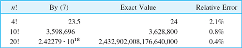
For large n the function is very large (see Table A3 in App. 5). A convenient approximation for large n is the Stirling formula2
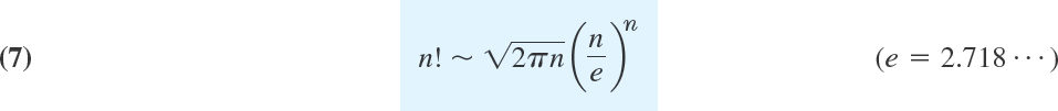
where ∼ is read “asymptotically equal” and means that the ratio of the two sides of (7) approaches 1 as n approaches infinity.
Binomial Coefficients
The binomial coefficients are defined by the formula

The numerator has k factors. Furthermore, we define

For integer a = n we obtain from (8)

Binomial coefficients may be computed recursively, because

Formula (8) also yields

There are numerous further relations; we mention two important ones,

and

Note the large numbers in the answers to some of these problems, which would make counting cases hopeless!
- In how many ways can a company assign 10 drivers to n buses, one driver to each bus and conversely?
- List (a) all permutations, (b) all combinations without repetitions, (c) all combinations with repetitions, of 5 letters a, e, i, o, u taken 2 at a time.
- If a box contains 4 rubber gaskets and 2 plastic gaskets, what is the probability of drawing (a) first the plastic and then the rubber gaskets, (b) first the rubber and then the plastic ones? Do this by using a theorem and checking it by multiplying probabilities.
- An urn contains 2 green, 3 yellow, and 5 red balls. We draw 1 ball at random and put it aside. Then we draw the next ball, and so on. Find the probability of drawing at first the 2 green balls, then the 3 yellow ones, and finally the red ones.
- In how many different ways can we select a committee consisting of 3 engineers, 2 physicists, and 2 computer scientists from 10 engineers, 5 physicists, and 6 computer scientists? First guess.
- How many different samples of 4 objects can we draw from a lot of 50?
- Of a lot of 10 items, 2 are defective. (a) Find the number of different samples of 4. Find the number of samples of 4 containing (b) no defectives, (c) 1 defective, (d) 2 defectives.
- Determine the number of different bridge hands. (A bridge hand consists of 13 cards selected from a full deck of 52 cards.)
- In how many different ways can 6 people be seated at a round table?
- If a cage contains 100 mice, 3 of which are male, what is the probability that the 3 male mice will be included if 10 mice are randomly selected?
- How many automobile registrations may the police have to check in a hit-and-run accident if a witness reports KDP7 and cannot remember the last two digits on the license plate but is certain that all three digits were different?
- If 3 suspects who committed a burglary and 6 innocent persons are lined up, what is the probability that a witness who is not sure and has to pick three persons will pick the three suspects by chance? That the witness picks 3 innocent persons by chance?
- CAS PROJECT. Stirling formula. (a) Using (7), compute approximate values of n! for n = 1, …, 20.
- (b) Determine the relative error in (a). Find an empirical formula for that relative error.
- (c) An upper bound for that relative error is e1/12n − 1. Try to relate your empirical formula to this.
- (d) Search through the literature for further information on Stirling's formula. Write a short eassy about your findings, arranged in logical order and illustrated with numeric examples.
- 14. TEAM PROJECT. Permutations, Combinations.
- Prove Theorem 2.
- Prove the last statement of Theorem 3.
- Derive (11) from (8).
- By the binomial theorem,
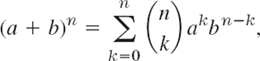
so that akbn−k has the coefficient
 . Can you conclude this from Theorem 3 or is this a mere coincidence?
 - Prove (14) by using the binomial theorem.
- Collect further formulas for binomial coefficients from the literature and illustrate them numerically.
- 15. Birthday problem. What is the probability that in a group of 20 people (that includes no twins) at least two have the same birthday, if we assume that the probability of having birthday on a given day is 1/365 for every day. First guess. Hint. Consider the complementary event.
24.5 Random Variables. Probability Distributions
In Sec. 24.1 we considered frequency distributions of data. These distributions show the absolute or relative frequency of the data values. Similarly, a probability distribution or, briefly, a distribution, shows the probabilities of events in an experiment. The quantity that we observe in an experiment will be denoted by X and called a random variable (orstochastic variable) because the value it will assume in the next trial depends on chance, on randomness—if you roll a die, you get one of the numbers from 1 to 6, but you don't know which one will show up next. Thus X = Number a die turns up is a random variable. So is X = Elasticity of rubber (elongation at break). (“Stochastic” means related to chance.)
If we count (cars on a road, defective screws in a production, tosses until a die shows the first Six), we have a discrete random variable and distribution. If we measure (electric voltage, rainfall, hardness of steel), we have a continuous random variable and distribution. Precise definitions follow. In both cases the distribution of X is determined by the distribution function

this is the probability that in a trial, X will assume any value not exceeding x.
CAUTION! The terminology is not uniform. F(x) is sometimes also called the cumulative distribution function.
For (1) to make sense in both the discrete and the continuous case we formulate conditions as follows.
A random variable X is a function defined on the sample space S of an experiment. Its values are real numbers. For every number a the probability
![]()
with which X assumes a is defined. Similarly, for any interval I the probability
![]()
with which X assumes any value in I is defined.
Although this definition is very general, in practice only a very small number of distributions will occur over and over again in applications.
From (1) we obtain the fundamental formula for the probability corresponding to an interval a < x ![]() b,
b,

This follows because X ![]() a (“X assumes any value not exceeding a”) and a < X
a (“X assumes any value not exceeding a”) and a < X ![]() b (“X assumes any value in the interval a < x
b (“X assumes any value in the interval a < x ![]() b”) are mutually exclusive events, so that by (1) and Axiom 3 of Definition 2 in Sec. 24.3 and subtraction of on both sides gives (2).
b”) are mutually exclusive events, so that by (1) and Axiom 3 of Definition 2 in Sec. 24.3 and subtraction of on both sides gives (2).
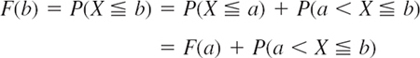
and subtraction of F(a) on both sides gives (2).
Discrete Random Variables and Distributions
By definition, a random variable X and its distribution are discrete if X assumes only finitely many or at most countably many values x1, x2, x3, …, called the possible values of X, with positive probabilities p1 = P(X = x1), p2 = P(X = x2), p3 = P(X = x3), …, whereas the probability P(X ∈ I) is zero for any interval I containing no possible value.
Clearly, the discrete distribution of X is also determined by the probability function f(x) of X, defined by
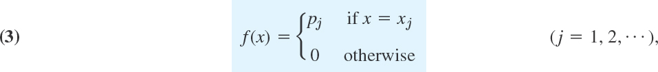
From this we get the values of the distribution function F(x) by taking sums,
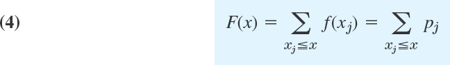
where for any given x we sum all the probabilities pj for which xj is smaller than or equal to that of x. This is a step function with upward jumps of size pj at the possible values Xj of X and constant in between.
EXAMPLE 1 Probability Function and Distribution Function
Figure 513 shows the probability function f(x) and the distribution function F(x) of the discrete random variable
![]()
X has the possible values x = 1, 2, 3, 4, 5, 6 with probability 1/6 each. At these x the distribution function has upward jumps of magnitude 1/6. Hence from the graph of f(x) we can construct the graph of F(x) and conversely.
In Figure 513 (and the next one) at each jump the fat dot indicates the function value at the jump!
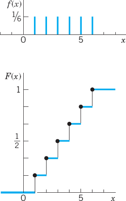
Fig. 513. Probability function f(x) and distribution function F (x) of the random variable X = Number obtained in tossing a fair die once

Fig. 514. Probability function f(x) and distribution function F (x) of the random variable X = Sum of the two numbers obtained in tossing two fair dice once
EXAMPLE 2 Probability Function and Distribution Function
The random variable X = Sum of the two numbers two fair dice turn up is discrete and has the possible values 2 (= 1 + 1), 3, 4, …, 12 (= 6 · 6). There are 6 · 6 = 36 equally likely outcomes (1, 1) (1, 2), …, (6, 6), where the first number is that shown on the first die and the second number that on the other die. Each such outcome has probability 1/36. Now X = 2 occurs in the case of the outcome (1, 1); X = 3 in the case of the two outcomes (1, 2) and (2, 1); X = 4 in the case of the three outcomes (1, 3), (2, 2), (3, 1); and so on. Hence f(x) = P(X = x) and F(x) = P(X ![]() x) have the values
x) have the values

Figure 514 shows a bar chart of this function and the graph of the distribution function, which is again a step function, with jumps (of different height!) at the possible values of X.
Two useful formulas for discrete distributions are readily obtained as follows. For the probability corresponding to intervals we have from (2) and (4)

This is the sum of all probabilities pj for which xj satisfies a < xj ![]() b. (Be careful about < and
b. (Be careful about < and ![]() !) From this and P(S) = 1 (Sec. 24.3) we obtain the following formula.
!) From this and P(S) = 1 (Sec. 24.3) we obtain the following formula.

EXAMPLE 3 Illustration of Formula (5)
In Example 2, compute the probability of a sum of at least 4 and at most 8.
Solution. ![]() .
.
EXAMPLE 4 Waiting Time Problem. Countably Infinite Sample Space
In tossing a fair coin, let X = Number of trials until the first head appears. Then, by independence of events (Sec. 24.3),
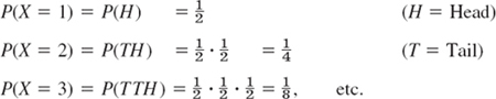
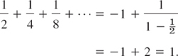
and in general ![]() , n = 1, 2, …. Also, (6) can be confirmed by the sum formula for the geometric series,
, n = 1, 2, …. Also, (6) can be confirmed by the sum formula for the geometric series,
Continuous Random Variables and Distributions
Discrete random variables appear in experiments in which we count (defectives in a production, days of sunshine in Chicago, customers standing in a line, etc.). Continuous random variables appear in experiments in which we measure (lengths of screws, voltage in a power line, Brinell hardness of steel, etc.). By definition, a random variable X and its distribution are of continuous type or, briefly, continuous, if its distribution function F(x) [defined in (1)] can be given by an integral
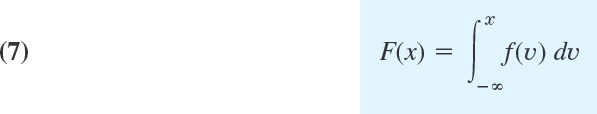
(we write ν because x is needed as the upper limit of the integral) whose integrand f(x), called the density of the distribution, is nonnegative, and is continuous, perhaps except for finitely many x-values. Differentiation gives the relation of f to F as
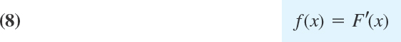
for every x at which f(x) is continuous.
From (2) and (7) we obtain the very important formula for the probability corresponding to an interval:

This is the analog of (5).
From (7) and P(S) = 1 (Sec. 24.3) we also have the analog of (6):

Continuous random variables are simpler than discrete ones with respect to intervals. Indeed, in the continuous case the four probabilities corresponding to a < X ![]() b, a < X < b, a
b, a < X < b, a ![]() X < b, and a
X < b, and a ![]() X
X ![]() b with any fixed a and b (> a) are all the same. Can you see why? (Answer. This probability is the area under the density curve, as in Fig. 515, and does not change by adding or subtracting a single point in the interval of integration.) This is different from the discrete case! (Explain.)
b with any fixed a and b (> a) are all the same. Can you see why? (Answer. This probability is the area under the density curve, as in Fig. 515, and does not change by adding or subtracting a single point in the interval of integration.) This is different from the discrete case! (Explain.)
The next example illustrates notations and typical applications of our present formulas.
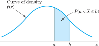
Fig. 515. Example illustrating formula (9)
EXAMPLE 5 Continuous Distribution
Let X have the density function f(x) = 0.75(1 − x)2 if −1 ![]() x
x ![]() 1 and zero otherwise. Find the distribution function. Find the probabilities
1 and zero otherwise. Find the distribution function. Find the probabilities ![]() and
and ![]() . Find x such that P(X
. Find x such that P(X ![]() x) = 0.95.
x) = 0.95.
Solution. From (7) we obtain F(x) = 0 if x ![]() −1,
−1,

and F(x) = 1 if x > 1. From this and (9) we get
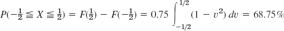
(because ![]() for a continuous distribution) and
for a continuous distribution) and
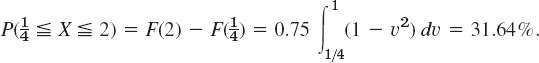
(Note that the upper limit of integration is 1, not 2. Why?) Finally,
![]()
Algebraic simplification gives 3x − x3 = 1.8. A solution is x = 0.73, approximately.
Sketch f(x) and mark ![]() , and 0.73, so that you can see the results (the probabilities) as areas under the curve. Sketch also F(x).
, and 0.73, so that you can see the results (the probabilities) as areas under the curve. Sketch also F(x).
Further examples of continuous distributions are included in the next problem set and in later sections.
- Graph the probability function f(x) = kx2 (x = 1, 2, 3, 4, 5; k suitable) and the distribution function.
- Graph the density function f(x) = kx2 (0 x 5; k suitable) and the distribution function.
- Uniform distribution. Graph f and F when the density of X is f(x) = k = const if −2 x 2 and 0 else-where. Find P(0 X 2).
- In Prob. 3 find c and
 such that P(−c < X < c) = 95% and P(0 < X < ) = 95%.
 - Graph f and F when
 ,
,  . Can f have further positive values?
 - A box contains 4 right-handed and 6 left-handed screws. Two screws are drawn at random without replacement. Let X be the number of left-handed screws drawn. Find the probabilities P(X = 0), P(X = 1), P(X = 2), P(1 < X 2), P(X 1), P(X
 1), P(X > 1), and P(0.5 < X < 10).
 - Let X be the number of years before a certain kind of pump needs replacement. Let X have the probability function f(x) = kx3, x = 0, 1, 2, 3, 4, Find k. Sketch f and F.
- Graph the distribution function F(x) = 1 − e−3x if x > 0, F(x) = 0 if x 0, and the density f(x). Find x such that F(x) = 0.9.
- Let X [millimeters] be the thickness of washers. Assume that X has the density f(x) = kx if 0.9 < x < 1.1 and 0 otherwise. Find k. What is the probability that a washer will have thickness between 0.95 mm and 1.05 mm?
- If the diameter X of axles has the density f(x) = k if 119.9 x 120.1 and 0 otherwise, how many defectives will a lot of 500 axles approximately contain if defectives are axles slimmer than 119.91 or thicker than 120.09?
- Find the probability that none of three bulbs in a traffic signal will have to be replaced during the first 1500 hours of operation if the lifetime X of a bulb is a random variable with the density f(x) = 6[0.25 − (x − 1.5)2] when 1 x 2 and f(x) = 0 otherwise, where x is measured in multiples of 1000 hours.
- Let X be the ratio of sales to profits of some company. Assume that X has the distribution function F(x) = 0 if x < 2, F(x) = (x2 − 4)/5 if 2 x < 3, F(x) = 1 if x 3. Find and sketch the density. What is the probability that X is between 2.5 (40% profit) and 5 (20% profit)?
- Suppose that in an automatic process of filling oil cans, the content of a can (in gallons) is Y = 100 + X, where X is a random variable with density f(x) = 1 − |x| when |x| 1 and 0 when |x| > 1. Sketch f(x) and F(x). In a lot of 1000 cans, about how many will contain 100 gallons or more? What is the probability that a can will contain less than 99.5 gallons? Less than 99 gallons?
- Find the probability function of X = Number of times a fair die is rolled until the first Six appears and show that it satisfies (6).
- Let X be a random variable that can assume every real value. What are the complements of the events X b, X < b, X c, X > c, b X c, b < X c?
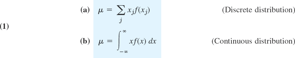
24.6 Mean and Variance of a Distribution
The mean μ and variance σ2 of a random variable X and of its distribution are the theoretical counterparts of the mean ![]() and variance s2 of a frequency distribution in Sec. 24.1 and serve a similar purpose. Indeed, the mean characterizes the central location and the variance the spread (the variability) of the distribution. The mean μ (mu) is defined by
and variance s2 of a frequency distribution in Sec. 24.1 and serve a similar purpose. Indeed, the mean characterizes the central location and the variance the spread (the variability) of the distribution. The mean μ (mu) is defined by
and the variance σ2 (sigma square) by
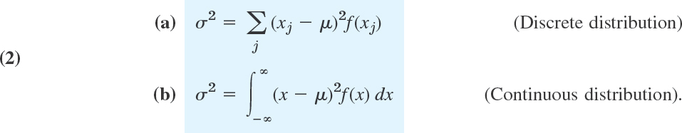
σ (the positive square root of σ2) is called the standard deviation of X and its distribution. f is the probability function or the density, respectively, in (a) and (b).
The mean μ is also denoted by E(X) and is called the expectation of X because it gives the average value of X to be expected in many trials. Quantities such as μ and σ2 that measure certain properties of a distribution are called parameters. μ and σ2 are the two most important ones. From (2) we see that
![]()
(except for a discrete “distribution” with only one possible value, so that σ2 = 0). We assume that μ and σ2 exist (are finite), as is the case for practically all distributions that are useful in applications.
The random variable X = Number of heads in a single toss of a fair coin has the possible values X = 0 and X = 1 with probabilities ![]() and
and ![]() . From (la) we thus obtain the mean
. From (la) we thus obtain the mean ![]() and (2a) yields the variance
and (2a) yields the variance
![]()
EXAMPLE 2 Uniform Distribution. Variance Measures Spread
The distribution with the density
![]()
and f = 0 otherwise is called the uniform distribution on the interval a < x < b. From (1b) (or from Theorem 1, below) we find that μ = (a + b)/2, and (2b) yields the variance
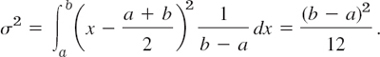
Figure 516 illustrates that the spread is large if and only if σ2 is large.
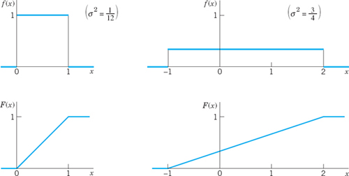
Fig. 516. Uniform distributions having the same mean (0.5) but different variances σ2
Symmetry. We can obtain the mean μ without calculation if a distribution is symmetric. Indeed, you may prove
THEOREM 1 Mean of a Symmetric Distribution
If a distribution is symmetric with respect to x = c, that is, f(c − x) = f(c + x), then μ = c. (Examples 1 and 2 illustrate this.)
Transformation of Mean and Variance
Given a random variable X with mean μ and variance σ2, we want to calculate the mean and variance of X* = a1 + a2X, where a1 and a2 are given constants. This problem is important in statistics, where it often appears.
THEOREM 2 Transformation of Mean and Variance
(a) If a random variable X has mean μ and variance σ2, then the random variable
![]()
has the mean μ* and variance σ*2, where
![]()
(b) In particular, the standardized random variable Z corresponding to X, given by

has the mean 0 and the variance 1.
PROOF
We prove (5) for a continuous distribution. To a small interval I of length Δx on the x-axis there corresponds the probability f(x)Δx [approximately; the area of a rectangle of base Δx and height f(x)]. Then the probability f(x)Δx must equal that for the corresponding interval on the x*-axis, that is, f*(x*)Δx*, where f* is the density of X* and Δx* is the length of the interval on the x*-axis corresponding to I. Hence for differentials we have f*(x*) dx* = f(x)dx. Also, x* = a1 + a2x by (4), so that (1b) applied to X* gives
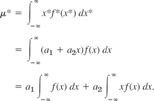
On the right the first integral equals 1, by (10) in Sec. 24.5. The second intergral is μ This proves (5) for μ*. It implies
![]()
From this and (2) applied to X*, again using f*(x*) dx* = f(x)dx, we obtain the second formula in (5),

For a discrete distribution the proof of (5) is similar.
Choosing a1 = −μ/σ and a2 = 1/σ we obtain (6) from (4), writing X* = Z. For these a1, a2 formula (5) gives μ* = 0 and σ*2 = 1, as claimed in (b).
Expectation, Moments
Recall that (1) defines the expectation (the mean) of X, the value of X to be expected on the average, written μ = E(X). More generally, if g(X) is nonconstant and continuous for all x, then is a random variable. Hence its mathematical expectation or, briefly, its expectation E(g(X)) is the value of g(X) to be expected on the average, defined [similarly to (1)] by

In the first formula, f is the probability function of the discrete random variable X. In the second formula, f is the density of the continuous random variable X. Important special cases are the kth moment of X (where k = 1, 2, …)
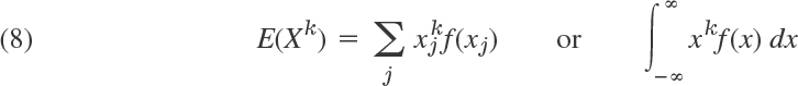
and the kth central moment of X (k = 1, 2, …)

This includes the first moment, the mean of X

It also includes the second central moment, the variance of X

For later use you may prove
![]()
1–8 MEAN, VARIANCE
Find the mean and variance of the random variable X with probability function or density f(x).
- f(x) = kx (0 x 2, k suitable)
- X = Number a fair die turns up
- Uniform distribution on [0, 2π]

- f(x) = 4e−4x (x 0)
- f(x) = k(1 − x2) if and 0 otherwise
- f(x) = Ce−x/2 (x = 0)
- X = Number of times a fair coin is flipped until the first Head appears. (Calculate μ only.)
- If the diameter X [cm] of certain bolts has the density f(x) = k(x − 0.9)(1.1 − x) for 0.9 < x < 1.1 and 0 for other x, what are k, μ and σ2? Sketch f(x).
- If, in Prob. 9, a defective bolt is one that deviates from 1.00 cm by more than 0.06 cm, what percentage of defectives should we expect?
- For what choice of the maximum possible deviation from 1.00 cm shall we obtain defectives in Probs. 9 and 10?
- What total sum can you expect in rolling a fair die 20 times? Do the experiment. Repeat it a number of times and record how the sum varies.
- What is the expected daily profit if a store sells X air conditioners per day with probability f(10) = 0.1, f(11) = 0.3, f(12) = 0.4, f(13) = 0.2 and the profit per conditioner is $55?
- Find the expectation of g(X) = X2, where X is uniformly distributed on the interval −1 x 1.
- A small filling station is supplied with gasoline every Saturday afternoon. Assume that its volume X of sales in ten thousands of gallons has the probability density f(x) = 6x(1 − x) if 0 x 1 and 0 otherwise. Determine the mean, the variance, and the standardized variable.
- What capacity must the tank in Prob. 15 have in order that the probability that the tank will be emptied in a given week be 5%?
- James rolls 2 fair dice, and Harry pays k cents to James, where k is the product of the two faces that show on the dice. How much should James pay to Harry for each game to make the game fair?
- What is the mean life of a lightbulb whose life X [hours] has the density f(x) = 0.001e−0.001x (x 0)?
- Let X be discrete with probability function
 Find the expectation of X3.
 - TEAM PROJECT. Means, Variances, Expectations.
- Show that E(X − μ) = 0, σ2 = E(X2) − μ2.
- Prove (10)–(12).
- Find all the moments of the uniform distribution on an interval a x b.
- The skewness γ of a random variable X is defined by

Show that for a symmetric distribution (whose third central moment exists) the skewness is zero.
- Find the skewness of the distribution with density f(x) = xe−x when x > 0 and f(x) = 0 otherwise. Sketch f(x).
- Calculate the skewness of a few simple discrete distributions of your own choice.
- Find a nonsymmetric discrete distribution with 3 possible values, mean 0, and skewness 0.
24.7 Binomial, Poisson, and Hypergeometric Distributions
These are the three most important discrete distributions, with numerous applications.
Binomial Distribution
The binomial distribution occurs in games of chance (rolling a die, see below, etc.), quality inspection (e.g., counting of the number of defectives), opinion polls (counting number of employees favoring certain schedule changes, etc.), medicine (e.g., recording the number of patients who recovered on a new medication), and so on. The conditions of its occurrence are as follows.
We are interested in the number of times an event A occurs in n independent trials. In each trial the event A has the same probability P(A) = p. Then in a trial, A will not occur with probability q = 1 − p. In n trials the random variable that interests us is
![]()
X can assume the values 0, 1, …, n and we want to determine the corresponding probabilities. Now X = x means that A occurs in x trials and in n − x trials it does not occur. This may look as follows.

Here B = Ac is the complement of A, meaning that A does not occur (Sec. 24.2). We now use the assumption that the trials are independent, that is, they do not influence each other. Hence (1) has the probability (see Sec. 24.3 on independent events)
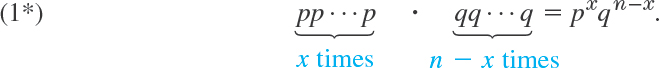
Now (1) is just one order of arranging x A’s and n − x B’s. We now use Theorem 1(b) in Sec. 24.4, which gives the number of permutations of n things (the n outcomes of the n trials) consisting of 2 classes, class 1 containing the n1 = x A’s and class 2 containing the n − n1 = n − x B’s. This number is

Accordingly, (1*), multiplied by this binomial coefficient, gives the probability P(X = x) of X = x, that is, of obtaining A precisely x times in n trials. Hence X has the probability function

and f(x) = 0 otherwise. The distribution of X with probability function (2) is called the binomial distribution or Bernoulli distribution. The occurrence of A is called success (regardless of what it actually is; it may mean that you miss your plane or lose your watch) and the nonoccurrence of A is called failure. Figure 517 shows typical examples. Numeric values can be obtained from Table A5 in App. 5 or from your CAS.
The mean of the binomial distribution is (see Team Project 16)

and the variance is (see Team Project 16)

For the symmetric case of equal chance of success and failure ![]() this gives the mean n/2, the variance n/4, and the probability function
this gives the mean n/2, the variance n/4, and the probability function
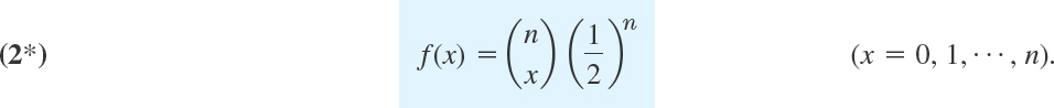
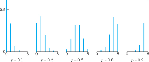
Fig. 517. Probability function (2) of the binomial distribution for n = 5 and various values of p
EXAMPLE 1 Binomial Distribution
Compute the probability of obtaining at least two “Six” in rolling a fair die 4 times.
Solution. ![]() The event “At least two ‘Six’” occurs if we obtain 2 or 3 or 4 “Six.” Hence the answer is
The event “At least two ‘Six’” occurs if we obtain 2 or 3 or 4 “Six.” Hence the answer is
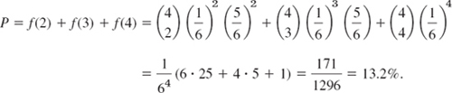
Poisson Distribution
The discrete distribution with infinitely many possible values and probability function

is called the Poisson distribution, named after S. D. Poisson (Sec. 18.5). Figure 518 shows (5) for some values of μ. It can be proved that this distribution is obtained as a limiting case of the binomial distribution, if we let p → 0 and n → ∞ so that the mean μ = np approaches a finite value. (For instance, μ = np may be kept constant.) The Poisson distribution has the mean μ and the variance (see Team Project 16)
![]()
Figure 518 gives the impression that, with increasing mean, the spread of the distribution increases, thereby illustrating formula (6), and that the distribution becomes more and more (approximately) symmetric.
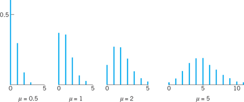
Fig. 518. Probability function (5) of the Poisson distribution for various values of μ
EXAMPLE 2 Poisson Distribution
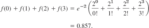
If the probability of producing a defective screw is p = 0.01, what is the probability that a lot of 100 screws will contain more than 2 defectives?
Solution. The complementary event is Ac: Not more than 2 defectives. For its probability we get, from the binomial distribution with mean μ = np = 1, the value [see (2)]
![]()
Since p is very small, we can approximate this by the much more convenient Poisson distribution with mean μ = np = 100 · 0.01 = 1, obtaining [see (5)]
Thus p(A) = 8.03%. Show that the binomial distribution gives p(A) = 7.94%, so that the Poisson approximation is quite good.
EXAMPLE 3 Parking Problems. Poisson Distribution
If on the average, 2 cars enter a certain parking lot per minute, what is the probability that during any given minute 4 or more cars will enter the lot?
Solution. To understand that the Poisson distribution is a model of the situation, we imagine the minute to be divided into very many short time intervals, let p be the (constant) probability that a car will enter the lot during any such short interval, and assume independence of the events that happen during those intervals. Then we are dealing with a binomial distribution with very large n and very small p, which we can approximate by the Poisson distribution with
![]()
because 2 cars enter on the average. The complementary event of the event “4 cars or more during a given minute” is “3 cars or fewer enter the lot” and has the probability
Answer: 14.3%. (Why did we consider that complement?)
Sampling with Replacement
This means that we draw things from a given set one by one, and after each trial we replace the thing drawn (put it back to the given set and mix) before we draw the next thing. This guarantees independence of trials and leads to the binomial distribution. Indeed, if a box contains N things, for example, screws, M of which are defective, the probability of drawing a defective screw in a trial is p = M/N. Hence the probability of drawing a nondefective screw is q = 1 − p = 1 − M/N, and (2) gives the probability of drawing x defectives in n trials in the form

Sampling without Replacement.
Hypergeometric Distribution
Sampling without replacement means that we return no screw to the box. Then we no longer have independence of trials (why?), and instead of (7) the probability of drawing x defectives in n trials is
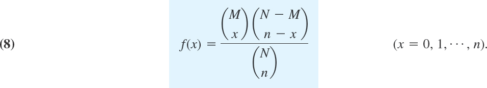
The distribution with this probability function is called the hypergeometric distribution (because its moment generating function (see Team Project 16) can be expressed by the hypergeometric function defined in Sec. 5.4, a fact that we shall not use).
Derivation of (8). By (4a) in Sec. 24.4 there are
 different ways of picking n things from N,
 different ways of picking x defectives from M,
 different ways of picking n − x nondefectives from N − M,
and each way in (b) combined with each way in (c) gives the total number of mutually exclusive ways of obtaining x defectives in n drawings without replacement. Since (a) is the total number of outcomes and we draw at random, each such way has the probability
![]() . From this, (8) follows.
. From this, (8) follows.
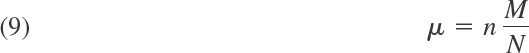
The hypergeometric distribution has the mean (Team Project 16)
and the variance

EXAMPLE 4 Sampling with and without Replacement
We want to draw random samples of two gaskets from a box containing 10 gaskets, three of which are defective. Find the probability function of the random variable X = Number of defectives in the sample.
Solution. We have N = 10, M = 3, N − M = 7, n = 2. For sampling with replacement, (7) yields

For sampling without replacement we have to use (8), finding

If N, M, and N − M are large compared with n, then it does not matter too much whether we sample with or without replacement, and in this case the hypergeometric distribution may be approximated by the binomial distribution (with p = M/N), which is somewhat
Hence, in sampling from an indefinitely large population (“infinite population”), we may use the binomial distribution, regardless of whether we sample with or without replacement.
- Mark the positions of μ in Fig. 517. Comment.
- Graph (2) for n = 8 as in Fig. 517 and compare with Fig. 517.
- In Example 3, if 5 cars enter the lot on the average, what is the probability that during any given minute 6 or more cars will enter? First guess. Compare with Example 3.
- How do the probabilities in Example 4 of the text change if you double the numbers: drawing 4 gaskets from 20, 6 of which are defective? First guess.
- Five fair coins are tossed simultaneously. Find the probability function of the random variable X = Number of heads and compute the probabilities of obtaining no heads, precisely 1 head, at least 1 head, not more than 4 heads.
- Suppose that 4% of steel rods made by a machine are defective, the defectives occurring at random during production. If the rods are packaged 100 per box, what is the Poisson approximation of the probability that a given box will contain x = 0, 1, …, 5 defectives?
- Let X be the number of cars per minute passing a certain point of some road between 8 A.M. and 10 A.M. on a Sunday. Assume that X has a Poisson distribution with mean 5. Find the probability of observing 4 or fewer cars during any given minute.
- Suppose that a telephone switchboard of some company on the average handles 300 calls per hour, and that the board can make at most 10 connections per minute. Using the Poisson distribution, estimate the probability that the board will be overtaxed during a given minute. (Use Table A6 in App. 5 or your CAS.)
- Rutherford–Geiger experiments. In 1910, E. Rutherford and H. Geiger showed experimentally that the number of alpha particles emitted per second in a radioactive process is a random variable X having a Poisson distribution. If X has mean 0.5, what is the probability of observing two or more particles during any given second?
- Let p = 2% be the probability that a certain type of lightbulb will fail in a 24-hour test. Find the probability that a sign consisting of 15 such bulbs will burn 24 hours with no bulb failures.
- Guess how much less the probability in Prob. 10 would be if the sign consisted of 100 bulbs. Then calculate.
- Suppose that a certain type of magnetic tape contains, on the average, 2 defects per 100 meters. What is the probability that a roll of tape 300 meters long will contain (a) x defects, (b) no defects?
- Suppose that a test for extrasensory perception consists of naming (in any order) 3 cards randomly drawn from a deck of 13 cards. Find the probability that by chance alone, the person will correctly name (a) no cards, (b) 1 card, (c) 2 cards, (d) 3 cards.
- If a ticket office can serve at most 4 customers per minute and the average number of customers is 120 per hour, what is the probability that during a given minute customers will have to wait? (Use the Poisson distribution, Table 6 in Appendix 5.)
- Suppose that in the production of 60-ohm radio resistors, nondefective items are those that have a resistance between 58 and 62 ohms and the probability of a resistor's being defective is 0.1%. The resistors are sold in lots of 200, with the guarantee that all resistors are nondefective. What is the probability that a given lot will violate this guarantee? (Use the Poisson distribution.)
- TEAM PROJECT. Moment Generating Function. The moment generating function G(t) is defined by

or
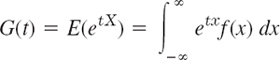
where X is a discrete or continuous random variable, respectively.
- Assuming that termwise differentiation and differentiation under the integral sign are permissible, show that E(Xk) = G(k)(0), where G(k) = dkG/dtk, in particular, μ = G′(0).
- Show that the binomial distribution has the moment generating function
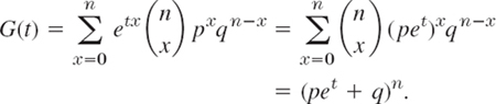
- Using (b), prove (3).
- Prove (4).
- Show that the Poisson distribution has the moment generating function
 and prove (6).
 - Prove
Using this, prove (9).
- 17. Multinomial distribution. Suppose a trial can result in precisely one of k mutually exclusive events A1, …, Ak with probabilities p1, … pk, respectively, p1 + … + pk = 1. where Suppose that n independent trials are performed. Show that the probability of getting x1 A1”s, …, xk Ak’s is

where 0
xj n, j = 1, …, k, and x1 + … + xk = n. The distribution having this probability function is called the multinomial distribution. - A process of manufacturing screws is checked every hour by inspecting n screws selected at random from that hour's production. If one or more screws are defective, the process is halted and carefully examined. How large should n be if the manufacturer wants the probability to be about 95% that the process will be halted when 10% of the screws being produced are defective? (Assume independence of the quality of any screw from that of the other screws.)
24.8 Normal Distribution
Turning from discrete to continuous distributions, in this section we discuss the normal distribution. This is the most important continuous distribution because in applications many random variables are normal random variables (that is, they have a normal distribution) or they are approximately normal or can be transformed into normal random variables in a relatively simple fashion. Furthermore, the normal distribution is a useful approximation of more complicated distributions, and it also occurs in the proofs of various statistical tests.
The normal distribution or Gauss distribution is defined as the distribution with the density
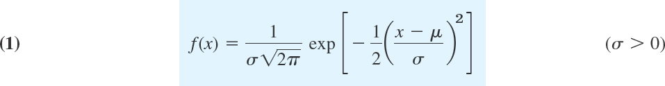
where exp is the exponential function with base e = 2.718 …. This is simpler than it may at first look. f(x) has these features (see also Fig. 519).
- μ is the mean and σ the standard deviation.
 is a constant factor that makes the area under the curve of f(x) from −∞ to ∞ equal to 1, as it must be by (10), Sec. 24.5.
- The curve of f(x) is symmetric with respect to x = μ because the exponent is quadratic. Hence for μ = 0 it is symmetric with respect to the y-axis x = 0 (Fig. 519, “bell-shaped curves”).
- The exponential function in (1) goes to zero very fast—the faster the smaller the standard deviation σ is, as it should be (Fig. 519).
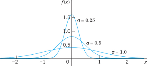
Fig. 519. Density (1) of the normal distribution with μ = 0 for various values of σ
Distribution Function F(x)
From (7) in Sec. 24.5 and (1) we see that the normal distribution has the distribution function
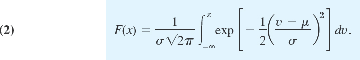
Here we needed x as the upper limit of integration and wrote ν (instead of x) in the integrand.
For the corresponding standardized normal distribution with mean 0 and standard deviation 1 we denote F(x) by Φ(z). Then we simply have from (2)
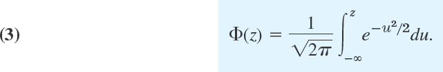
This integral cannot be integrated by one of the methods of calculus. But this is no serious handicap because its values can be obtained from Table A7 in App. 5 or from your CAS. These values are needed in working with the normal distribution. The curve of Φ(z) is S-shaped. It increases monotone (why?) from 0 to 1 and intersects the vertical axis at ![]() (why?), as shown in Fig. 520.
(why?), as shown in Fig. 520.
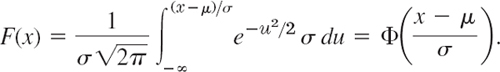
Relation Between F(x) and Φ(z). Although your CAS will give you values of F(x) in (2) with any μ and σ directly, it is important to comprehend that and why any such an F(x) can be expressed in terms of the tabulated standard Φ(z), as follows.
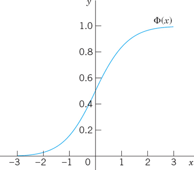
Fig. 520. Distribution function Φ(z) of the normal distribution with mean 0 and variance 1
THEOREM 1 Use of the Normal Table A7 in App. 5
The distribution function F(x) of the normal distribution with any μ and σ [see (2)] is related to the standardized distribution function Φ(z) in (3) by the formula

PROOF
Comparing (2) and (3) we see that we should set
![]()
as the new upper limit of integration. Also ν − μ = σu, thus dν = σ du. Together, since σ drops out,
Probabilities corresponding to intervals will be needed quite frequently in statistics in Chap. 25. These are obtained as follows.
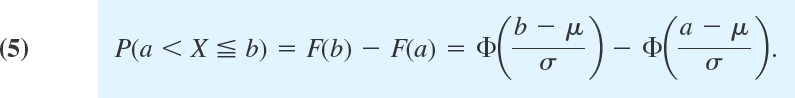
THEOREM 2 Normal Probabilities for Intervals
The probability that a normal random variable X with mean μ and standard deviation σ assume any value in an interval a < x ![]() b is
b is
PROOF
Formula (2) in Sec. 24.5 gives the first equality in (5), and (4) in this section gives the second equality.
Numeric Values
In practical work with the normal distribution it is good to remember that about ![]() of all values of X to be observed will lie between μ ± σ, about 95% between μ ± 2σ, and practically all between the three-sigma limits μ ± 3σ. More precisely, by Table A7 in App. 5,
of all values of X to be observed will lie between μ ± σ, about 95% between μ ± 2σ, and practically all between the three-sigma limits μ ± 3σ. More precisely, by Table A7 in App. 5,
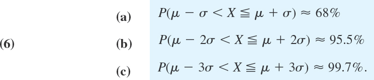
Formulas (6a) and (6b) are illustrated in Fig. 521.
The formulas in (6) show that a value deviating from μ by more than σ, 2σ, or 3σ will occur in one of about 3, 20, and 300 trials, respectively.

Fig. 521. Illustration of formula (6)
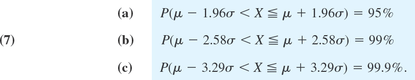
In tests (Chap. 25) we shall ask, conversely, for the intervals that correspond to certain given probabilities; practically most important are the probabilities of 95%, 99%, and 99.9%. For these, Table A8 in App. 5 gives the answers μ ± 2σ, μ ± 2.6σ, and μ ± 3.3σ, respectively. More precisely,
Working with the Normal Tables A7 and A8 in App. 5
There are two normal tables in App. 5, Tables A7 and A8. If you want probabilities, use Table A7. If probabilities are given and corresponding intervals or x-values are wanted, use Table A8. The following examples are typical. Do them with care, verifying all values, and don't just regard them as dull exercises for your software. Make sketches of the density to see whether the results look reasonable.
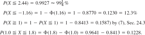
EXAMPLE 2 Probabilities for Given Intervals, Table A7
Let X be normal with mean 0.8 and variance 4 (so that σ = 2). Then by (4) and (5)
![]()
or, if you like it better, (similarly in the other cases)
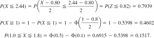
EXAMPLE 3 Unknown Values c for Given Probabilities, Table A8
Let X be normal with mean 5 and variance 0.04 (hence standard deviation 0.2). Find c or k corresponding to the given probability
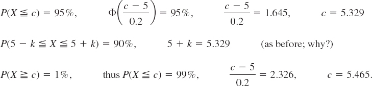
In a production of iron rods let the diameter X be normally distributed with mean 2 in. and standard deviation 0.008 in.
- What percentage of defectives can we expect if we set the tolerance limits at 2 ± 0.02 in.?
- How should we set the tolerance limits to allow for 4% defectives?
Solution. (a) ![]() because from (5) and Table A7 we obtain for the complementary event the probability
because from (5) and Table A7 we obtain for the complementary event the probability
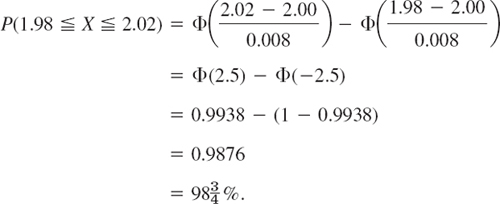
(b) 2 ± 0.0164 because, for the complementary event, we have
![]()
or
![]()
so that Table A8 gives
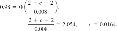
Normal Approximation of the Binomial Distribution
The probability function of the binomial distribution is (Sec. 24.7)

If n is large, the binomial coefficients and powers become very inconvenient. It is of great practical (and theoretical) importance that, in this case, the normal distribution provides a good approximation of the binomial distribution, according to the following theorem, one of the most important theorems in all probability theory.
THEOREM 3 Limit Theorem of De Moivre and Laplace
For large n,
![]()
Here f is given by (8). The function

is the density of the normal distribution with mean μ = np and variance σ2 = npq (the mean and variance of the binomial distribution). The symbol ~ (read asymptotically equal) means that the ratio of both sides approaches 1 as n approaches ∞. Furthermore, for any nonnegative integers a and b (> a),
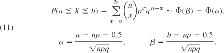
A proof of this theorem can be found in [G3] listed in App. 1. The proof shows that the term 0.5 in α and β is a correction caused by the change from a discrete to a continuous distribution.
- Let X be normal with mean 10 and variance 4. Find P(X > 12), P(X < 10), P(X < 11), P(9 < X < 13).
- Let X be normal with mean 105 and variance 25. Find P(X 112.5), P(x > 100), P(110.5) < X < 111.25).
- Let X be normal with mean 50 and variance 9. Determine c such that P(X < c) = 5%, P(X > c) = 1%, P(50 − c < X < 50 + c) = 50%.
- Let X be normal with mean 3.6 and variance 0.01. Find c such that P(X c) = 50%, P(X > c) = 10%, P(−c < X − 3.6 c) = 99.9%.
- If the lifetime X of a certain kind of automobile battery is normally distributed with a mean of 5 years and a standard deviation of 1 year, and the manufacturer wishes to guarantee the battery for 4 years, what percentage of the batteries will he have to replace under the guarantee?
- If the standard deviation in Prob. 5 were smaller, would that percentage be larger or smaller?
- A manufacturer knows from experience that the resistance of resistors he produces is normal with mean μ = 150 Ω and standard deviation σ = 5 Ω. What percentage of the resistors will have resistance between and Between 148 Ω and 152 Ω? Between 140 Ω and 160 Ω?
- The breaking strength X [kg] of a certain type of plastic block is normally distributed with a mean of 1500 kg and a standard deviation of 50 kg. What is the maximum load such that we can expect no more than 5% of the blocks to break?
- If the mathematics scores of the SAT college entrance exams are normal with mean 480 and standard deviation 100 (these are about the actual values over the past years) and if some college sets 500 as the minimum score for new students, what percent of students would not reach that score?
- A producer sells electric bulbs in cartons of 1000 bulbs. Using (11), find the probability that any given carton contains not more than 1% defective bulbs, assuming the production process to be a Bernoulli experiment with p = 1%(= probability that any given bulb will be defective). First guess. Then calculate.
- If sick-leave time X used by employees of a company in one month is (very roughly) normal with mean 1000 hours and standard deviation 100 hours, how much time t should be budgeted for sick leave during the next month if t is to be exceeded with probability of only 20%?
- If the monthly machine repair and maintenance cost X in a certain factory is known to be normal with mean $12,000 and standard deviation $2000, what is the probability that the repair cost for the next month will exceed the budgeted amount of $15,000?
- If the resistance X of certain wires in an electrical network is normal with mean 0.01 Ω and standard deviation 0.001 Ω, how many of 1000 wires will meet the specification that they have resistance between 0.009 and 0.011 Ω?
- TEAM PROJECT. Normal Distribution. (a) Derive the formulas in (6) and (7) from the appropriate normal table.
(b) Show that Φ(−z) = 1 − Φ(z). Give an example.
(c) Find the points of inflection of the curve of (1).
(d) Considering Φ2(∞) and introducing polar coordinates in the double integral (a standard trick worth remembering), prove

(e) Show that σ in (1) is indeed the standard deviation of the normal distribution. [Use (12).]
(f) Bernoulli's law of large numbers. In an experiment let an event A have probability P(0 < p < 1), and let X be the number of times A happens in n independent trials. Show that for any given ∈ > 0,
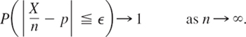
(g) Transformation. If X is normal with mean μ and variance σ2, show that X* = c1X + c2(c1 > 0) is normal with mean μ* = c1μ + c2 and variance
 .
. - WRITING PROJECT. Use of Tables, Use of CAS. Give a systematic discussion of the use of Tables A7 and A8 for obtaining P(X < b), P(X > a), P(a < X < b), P(X < c) = k, P(X > c) = k, as well as P(μ − c < X < μ + c) = k; include simple examples. If you have a CAS, describe to what extent it makes the use of those tables superfluous; give examples.
24.9 Distributions of Several Random Variables
Distributions of two or more random variables are of interest for two reasons:
1. They occur in experiments in which we observe several random variables, for example, carbon content X and hardness Y of steel, amount of fertilizer X and yield of corn Y, height X1, weight X2, and blood pressure X3 of persons, and so on.
2. They will be needed in the mathematical justification of the methods of statistics in Chap. 25.
In this section we consider two random variables X and Y or, as we also say, a two-dimensional random variable (X, Y). For (X, Y) the outcome of a trial is a pair of numbers X = x, Y = y, briefly (X, Y) = (x, y), which we can plot as a point in the XY-plane.
The two-dimensional probability distribution of the random variable (X, Y) is given by the distribution function

This is the probability that in a trial, X will assume any value not greater than x and in the same trial, Y will assume any value not greater than y. This corresponds to the blue region in Fig. 522, which extends to −∞ to the left and below. F(x, y) determines the

probability distribution uniquely, because in analogy to formula (2) in Sec. 24.5, that is, P(a < X ![]() b) = F(b) − F(a), we now have for a rectangle (see Prob. 16)
b) = F(b) − F(a), we now have for a rectangle (see Prob. 16)
![]()
As before, in the two-dimensional case we shall also have discrete and continuous random variables and distributions.
Discrete Two-Dimensional Distributions
In analogy to the case of a single random variable (Sec. 24.5), we call (X, Y) and its distribution discrete if (X, Y) can assume only finitely many or at most countably infinitely many pairs of values (x1, y1), (x2, y2), … with positive probabilities, whereas the probability for any domain containing none of those values of (X, Y) is zero.
Let (xj, yj) be any of those pairs and let P(X = xi, Y = yj) = pij (where we admit that pij may be 0 for certain pairs of subscripts i, j). Then we define the probability function f(x, y) of (X, Y) by
![]()
here, i = 1, 2, … and j = 1, 2, … independently. In analogy to (4), Sec. 24.5, we now have for the distribution function the formula

Instead of (6) in Sec. 24.5 we now have the condition
EXAMPLE 1 Two-Dimensional Discrete Distribution
If we simultaneously toss a dime and a nickel and consider
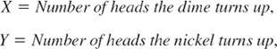
then X and Y can have the values 0 or 1, and the probability function is
![]()
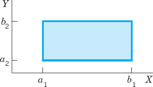
Fig. 523. Notion of a two-dimensional distribution
Continuous Two-Dimensional Distributions
In analogy to the case of a single random variable (Sec. 24.5) we call (X, Y) and its distribution continuous if the corresponding distribution function F(x, y) can be given by a double integral

whose integrand f, called the density of (X, Y), is nonnegative everywhere, and is continuous, possibly except on finitely many curves.
From (6) we obtain the probability that (X, Y) assume any value in a rectangle (Fig. 523) given by the formula
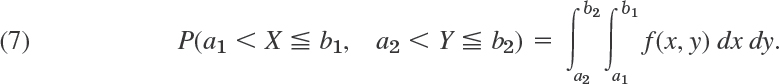
EXAMPLE 2 Two-Dimensional Uniform Distribution in a Rectangle
Let R be the rectangle α1 < x ![]() β1, α2 < y
β1, α2 < y ![]() β2. The density (see Fig. 524)
β2. The density (see Fig. 524)
![]()
defines the so-called uniform distribution in the rectangle R; here k = (β1 − α1)(β2 − α2) is the area of R. The distribution function is shown in Fig. 525.

Fig. 524. Density function (8) of the uniform distribution
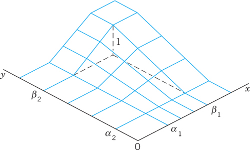
Fig. 525. Distribution function of the uniform distribution defined by (8)
Marginal Distributions of a Discrete Distribution
This is a rather natural idea, without counterpart for a single random variable. It amounts to being interested only in one of the two variables in (X, Y), say, X, and asking for its distribution, called the marginal distribution of X in (X, Y). So we ask for the probability P (X = x, Y arbitrary). Since (X, Y) is discrete, so is X. We get its probability function, call it f1(x), from the probability function f(x, y) of (X, Y) by summing over y:

where we sum all the values of f(x, y) that are not 0 for that x.
From (9) we see that the distribution function of the marginal distribution of X is

Similarly, the probability function
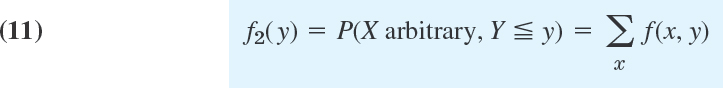
determines the marginal distribution of Y in (X, Y). Here we sum all the values of f(x, y) that are not zero for the corresponding y. The distribution function of this marginal distribution is

EXAMPLE 3 Marginal Distributions of a Discrete Two-Dimensional Random Variable
In drawing 3 cards with replacement from a bridge deck let us consider
![]()
The deck has 52 cards. These include 4 queens, 4 kings, and 4 aces. Hence in a single trial a queen has probability ![]() and a king or ace
and a king or ace ![]() . This gives the probability function of (X, Y),
. This gives the probability function of (X, Y),

and f(x, y) = 0 otherwise. Table 24.1 shows in the center the values of f(x, y) and on the right and lower margins the values of the probability functions f1(x) and f2(y) of the marginal distributions of X and Y, respectively.
Table 24.1 Values of the Probability Functions f(x, y), f1(x), f2(y) in Drawing Three Cards with Replacement from a Bridge Deck, where X is the Number of Queens Drawn and Y is the Number of Kings or Aces Drawn
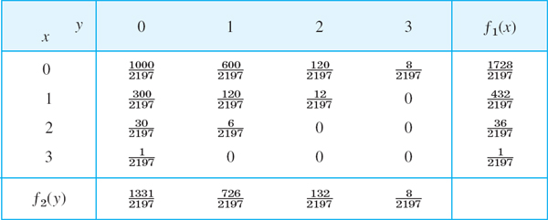
Marginal Distributions of a Continuous Distribution
This is conceptually the same as for discrete distributions, with probability functions and sums replaced by densities and integrals. For a continuous random variable (X, Y) with density f(x, y) we now have the marginal distribution of X in (X, Y), defined by the distribution function

with the density f1 of X obtained from f(x, y) by integration over y,
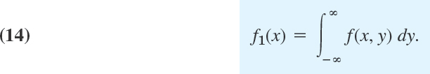
Interchanging the roles of X and Y, we obtain the marginal distribution of Y in (X, Y) with the distribution function

and density

Independence of Random Variables
X and Y in a (discrete or continuous) random variable (X, Y) are said to be independent if

holds for all (x, y) Otherwise these random variables are said to be dependent. These definitions are suggested by the corresponding definitions for events in Sec. 24.3.
Necessary and sufficient for independence is

for all x and y. Here the f’s are the above probability functions if (X, Y) is discrete or those densities if (X, Y) is continuous. (See Prob. 20.)
EXAMPLE 4 Independence and Dependence
In tossing a dime and a nickel, X = Number of heads on the dime, Y = Number of heads on the nickel may assume the values 0 or 1 and are independent. The random variables in Table 24.1 are dependent.
Extension of Independence to n-Dimensional Random Variables. This will be needed throughout Chap. 25. The distribution of such a random variable X = (X1, …, Xn) is determined by a distribution function of the form
![]()
The random variables X1, …, Xn are said to be independent if
![]()
for all (x1, …, xn). Here Fj(xj) is the distribution function of the marginal distribution of Xj in X, that is,
![]()
Otherwise these random variables are said to be dependent.
Functions of Random Variables
When n = 2, we write X1 = X, X2 = Y, x1 = x,x2 = y. Taking a nonconstant continuous function g(x, y) defined for all x, y, we obtain a random variable Z = g(X, Y). For example, if we roll two dice and X and Y are the numbers the dice turn up in a trial, then Z = X + Y is the sum of those two numbers (see Fig. 514 in Sec. 24.5).
In the case of a discrete random variable (X, Y) we may obtain the probability function f(z) of Z = g(X, Y) by summing all f(x, y) for which g(x, y) equals the value of z considered; thus

Hence the distribution function of Z is

where we sum all values of f(x, y) for which g(x, y) ![]() z.
z.
In the case of a continuous random variable (X, Y) we similarly have
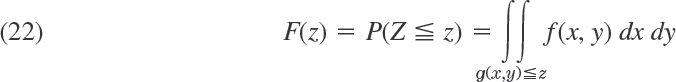
where for each z we integrate the density f(x, y) of (X, Y) over the region g(x, y) ![]() z in the xy-plane, the boundary curve of this region being g(x, y) = z.
z in the xy-plane, the boundary curve of this region being g(x, y) = z.
Addition of Means
The number
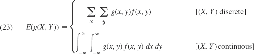
is called the mathematical expectation or, briefly, the expectation of g(X, Y). Here it is assumed that the double series converges absolutely and the integral of |g(x, y)|f(x, y) over the xy-plane exists (is finite). Since summation and integration are linear processes, we have from (23)
![]()
An important special case is
![]()
and by induction we have the following result.
The mean (expectation) of a sum of random variables equals the sum of the means (expectations) , that is,

Furthermore, we readily obtain
THEROEM 2 Multiplication of Means
The mean (expectation) of the product of independent random variables equals the product of the means (expectations) , that is,
![]()
PROOF
If X and Y are independent random variables (both discrete or both continuous), then E(XY) = E(X)E(Y). In fact, in the discrete case we have
![]()
and in the continuous case the proof of the relation is similar. Extension to n independent random variables gives (26), and Theorem 2 is proved.
Addition of Variances
This is another matter of practical importance that we shall need. As before, let Z =X + Y and denote the mean and variance of Z by μ and σ2. Then we first have (see Team Project 20(a) in Problem Set 24.6)
![]()
From (24) we see that the first term on the right equals
![]()
For the second term on the right we obtain from Theorem 1
![]()
By substituting these expressions into the formula for σ2 we have
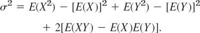
From Team Project 20, Sec. 24.6, we see that the expression in the first line on the right is the sum of the variances of X and Y, which we denote by ![]() and
and ![]() , respectively. The quantity in the second line (except for the factor 2) is
, respectively. The quantity in the second line (except for the factor 2) is

and is called the covariance of X and Y. Consequently, our result is
![]()
If X and Y are independent, then
![]()
hence σXY = 0, and
![]()
Extension to more than two variables gives the basic
THEOREM 3 Addition of Variances
The variance of the sum of independent random variables equals the sum of the variances of these variables.
CAUTION! In the numerous applications of Theorems 1 and 3 we must always remember that Theorem 3 holds only for independent variables.
This is the end of Chap. 24 on probability theory. Most of the concepts, methods, and special distributions discussed in this chapter will play a fundamental role in the next chapter, which deals with methods of statistical inference, that is, conclusions from samples to populations, whose unknown properties we want to know and try to discover by looking at suitable properties of samples that we have obtained.
- Let f(x, y) = k when 8 x 12 and 0 y 2 and zero elsewhere. Find k. Find P(X 11, 1 Y 1.5) and p(9 X 13, Y 1).
- Find P(X > 4, Y > 4) and P(X 1, Y 1) if (X, Y) has the density
 if x 0, y 0, x + y 8.
 - Let f(x, y) = k if x > 0, y > 0, x + y < 3 and 0 otherwise. Find k. Sketch f(x, y). Find P(X + Y 1), P(Y > X).
- Find the density of the marginal distribution of X in Prob. 2.
- Find the density of the marginal distribution of Y in Fig. 524.
- If certain sheets of wrapping paper have a mean weight of 10 g each, with a standard deviation of 0.05 g, what are the mean weight and standard deviation of a pack of 10,000 sheets?
- What are the mean thickness and the standard deviation of transformer cores each consisting of 50 layers of sheet metal and 49 insulating paper layers if the metal sheets have mean thickness 0.5 mm each with a standard deviation of 0.05 mm and the paper layers have mean 0.05 mm each with a standard deviation of 0.02 mm?
- Let X [cm] and Y [cm] be the diameters of a pin and hole, respectively. Suppose that (X, Y) has the density

and 0 otherwise. (a) Find the marginal distributions. (b) What is the probability that a pin chosen at random will fit a hole whose diameter is 1.00?
- Using Theorems 1 and 3, obtain the formulas for the mean and the variance of the binomial distribution.
- Using Theorem 1, obtain the formula for the mean of the hypergeometric distribution. Can you use Theorem 3 to obtain the variance of that distribution?
- A 5-gear assembly is put together with spacers between the gears. The mean thickness of the gears is 5.020 cm with a standard deviation of 0.003 cm. The mean thickness of the spacers is 0.040 cm with a standard deviation of 0.002 cm. Find the mean and standard deviation of the assembled units consisting of 5 randomly selected gears and 4 randomly selected spacers.
- If the mean weight of certain (empty) containers is 5 lb the standard deviation is 0.2 lb, and if the filling of the containers has mean weight 100 lb and standard deviation 0.5 lb, what are the mean weight and the standard deviation of filled containers?
- Find P(X > Y) when (X, Y) has the density

and 0 otherwise.
- An electronic device consists of two components. Let X and Y [years] be the times to failure of the first and second components, respectively. Assume that (X, Y) has the density f(x, y) = 4e−2(x+y) if x > 0 and y > 0 and 0 otherwise. (a) Are X and Y dependent or independent? (b) Find the densities of the marginal distributions. (c) What is the probability that the first component will have a lifetime of 2 years or longer?
- Give an example of two different discrete distributions that have the same marginal distributions.
- Prove (2).
- Let (X, Y) have the probability function
Are X and Y independent?
- Let (X, Y) have the density
and 0 otherwise. Determine k. Find the densities of the marginal distributions. Find the probability

- Show that the random variables with the densities

and

if 0
x 1, 0 y 1 and f(x, y) = 0 and g(x, y) = 0 elsewhere, have the same marginal distribution. - Prove the statement involving (18).
CHAPTER 24 REVIEW QUESTIONS AND PROBLEMS
- What are stem-and-leaf plots? Boxplots? Histograms? Compare their advantages.
- What properties of data are measured by the mean? The median? The standard deviation? The variance?
- What do we mean by an experiment? An outcome? An event? Give examples.
- What is a random variable? Its distribution function? Its probability function or density?
- State the definition of probability from memory. Give simple examples.
- What is sampling with and without replacement? What distributions are involved?
- When is the Poisson distribution a good approximation of the binomial distribution? The normal distribution?
- Explain the use of the tables of the normal distribution. If you have a CAS, how would you proceed without the tables?
- State the main theorems on probability. Illustrate them by simple examples.
- State the most important facts about distributions of two random variables and their marginal distributions.
- Make a stem-and-leaf plot, histogram, and boxplot of the data 110, 113, 109, 118, 110, 115, 104, 111, 116, 113.
- Same task as in Prob. 11. for the data 13.5, 13.2, 12.1, 13.6, 13.3.
- Find the mean, standard deviation, and variance in Prob. 11.
- Find the mean, standard deviation, and variance in Prob. 12.
- Show that the mean always lies between the smallest and the largest data value.
- What are the outcomes in the sample space of the experiment of simultaneously tossing three coins?
- Plot a histogram of the data 8, 2, 4, 10 and guess and s by inspecting the histogram. Then calculate , s2, and s.
- Using a Venn diagram, show that A ⊆ B if and only if A ∩ B = A.
- Suppose that 3% of bolts made by a machine are defective, the defectives occurring at random during production. If the bolts are packaged 50 per box, what is the binomial approximation of the probability that a given box will contain x = 0, 1, …, 5 defectives?
- Of a lot of 12 items, 3 are defective. (a) Find the number of different samples of 3 items. Find the number of samples of 3 items containing (b) no defectives, (c) 1 defective, (d) 2 defectives, (e) 3 defectives.
- Find the probability function of X = Number of times of tossing a fair coin until the first head appears.
- If the life of ball bearings has the density f(x) = ke−x if 0 x 2 and 0 otherwise, what is k? What is the probability P(X 1)?
- Find the mean and variance of a discrete random variable X having the probability function
 ,
,  .
. - Let X be normal with mean 14 and variance 4. Determine c such that P(X c) = 95%, P(X c) = 5%, P(X c) = 99.5%.
- Let X be normal with mean 80 and variance 9. Find P(X > 83), P(X < 81), P(X < 80), and P (78 < X < 82).
SUMMARY OF CHAPTER 24
Data Analysis. Probability Theory
A random experiment, briefly called experiment, is a process in which the result (“outcome”) depends on “chance” (effects of factors unknown to us). Examples are games of chance with dice or cards, measuring the hardness of steel, observing weather conditions, or recording the number of accidents in a city. (Thus the word “experiment” is used here in a much wider sense than in common language.) The outcomes are regarded as points (elements) of a set S, called the sample space, whose subsets are called events. For events E we define a probability P(E) by the axioms (Sec. 24.3)
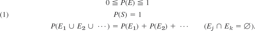
These axioms are motivated by properties of frequency distributions of data (Sec. 24.1).
The complement of Ec of E has the probability
![]()
The conditional probability of an event B under the condition that an event A happens is (Sec. 24.3)

Two events A and B are called independent if the probability of their simultaneous appearance in a trial equals the product of their probabilities, that is, if
![]()
With an experiment we associate a random variable X. This is a function defined on S whose values are real numbers; furthermore, X is such that the probability P(X = a) with which X assumes any value a, and the probability P(a < X ![]() b) with which X assumes any value in an interval a < X
b) with which X assumes any value in an interval a < X ![]() b are defined (Sec. 24.5). The probability distribution of X is determined by the distribution function
b are defined (Sec. 24.5). The probability distribution of X is determined by the distribution function
![]()
In applications there are two important kinds of random variables: those of the discrete type, which appear if we count (defective items, customers in a bank, etc.) and those of the continuous type, which appear if we measure (length, speed, temperature, weight, etc.).
A discrete random variable has a probability function
![]()
Its mean μ and variance σ2 are (Sec. 24.6)

where the xj are the values for which X has a positive probability. Important discrete random variables and distributions are the binomial, Poisson, and hypergeometric distributions discussed in Sec. 24.7.
A continuous random variable has a density
![]()
Its mean and variance are (Sec. 24.6)

Very important is the normal distribution (Sec. 24.8), whose density is

and whose distribution function is (Sec. 24.8; Tables A7, A8 in App. 5)

A two-dimensional random variable (X, Y) occurs if we simultaneously observe two quantities (for example, height X and weight Y of adults). Its distribution function is (Sec. 24.9)
![]()
X and Y have the distribution functions (Sec. 24.9)
![]()
respectively; their distributions are called marginal distributions. If both X and Y are discrete, then (X, Y) has a probability function
![]()
If both X and Y are continuous, then (X, Y) has a density f (x, y).