IN THIS CHAPTER
Formatting numbers
Changing text formatting
Using the formatting toolbar and palette
Using AutoFormat
Formatting conditionally
Applying styles
Using document themes
You've probably heard it said that quality is more important than quantity. In a way, this can apply to Excel worksheets. How your data is presented can be as important is what it says. In business, you can present reams of data to support your point of view, but if it's hard to read or poorly laid out, your audience is likely to tune out or get frustrated. Properly formatting your data not only helps make your worksheets easier for others to understand, it makes them easier to work with.
The designers of Excel have provided you with an array of formatting options for data and text. You can choose from a huge number of data formats, depending on the data and how you want it presented. Excel lets you format numbers in a variety of ways—as date and time values, currency, percentages, fractions, and more.
In addition to data formats, you can apply style formats to cells and worksheets. You can make changes to character and text formatting, altering fonts, sizes, and colors. You can format cell backgrounds as well, by changing colors, shading, and borders. You can even apply conditional formatting that automatically changes the way numbers are displayed depending on the values; for example, you can highlight negative values in red. You can even create and use styles and themes so you can reapply the same formatting options to other workbooks you create. In this chapter, you learn how you can apply formatting to cells and to your data in order to present your work in the best way possible.
The Format Cell dialog box, shown in Figure 14.1, is your one-stop-shopping place to set most cell formatting options, including number formats, text alignment, fonts, and borders and shading. You can activate it for a single cell at a time to customize its format, or more commonly, for a collection of cells, a row or column, or an entire worksheet or workbook. To activate the Format Cells dialog box, follow these steps:
Select the cell or cells that you want to format by doing one of the following:
Click an individual cell to select it.
Select multiple cells by pressing

Select an entire row or column by clicking the row or column header.
Select the entire worksheet using Control+A.
Choose Format
Cells, or press +1, or right-click the selection and choose Format Cells.
Note
Don't activate the Format Cells dialog box while in Edit mode. If you do so, you see only font formatting options. Make sure you are in Ready mode (as shown in the Status bar) in order to get all the formatting options available.

Excel's main purpose is to work with numbers, so it's no surprise that Excel is most flexible when giving you options for formatting them. Numbers are used to represent currency, dates and times, percentages, fractions, and more. If the provided formats aren't enough for you, you can define a custom format that should give you exactly what you need.
The first tab of the Format Cells dialog box is used to choose a data format for numbers in cells (or to set it to use no data formatting whatsoever). Click the Number tab to select number formatting, and choose a data format from the list. Most data types have additional formatting options, which you learn about in this section.
Tip
Note that setting a format for a cell doesn't change the underlying data; it only affects how it is presented. You can always see the actual data contained in a cell by double-clicking it (if the cell and worksheet are not protected), or by clicking it and viewing the data on the Formula bar.
The default format for cells is the first one on the list—the General format. When cells are formatted as General, Excel makes its best guess to display numbers and text. Numbers are generally displayed as they are typed, with a few exceptions. Figure 14.2 shows some examples of General formatting, and the following rules apply to General formatted numbers:
Numbers are aligned to the left, and text is aligned to the right.
Trailing zeros entered to the right of a decimal point are truncated.
Decimals entered without a number to the left of the decimal point are displayed with a single zero.
Leading zeros on numbers are removed.
Numbers are displayed using scientific notation if they contain ten or more digits.

You can go beyond Excel's automatic number formatting by choosing the Number data type. This data type lets you choose a consistent format to use to display numbers no matter how they are entered. Figure 14.3 shows the options available when using the Number format. You can set the following options:
Decimal places: Choose the number of digits to display after the decimal point. This can range from 0 to 30.
Use thousands separator: Checking this option causes Excel to display a separator character for every thousands value.
Negative numbers: Choose a conditional formatting option for negative numbers. Typical options are display with a negative sign, display in another color such as red, or display of the number inside parentheses.
Note
The decimal point, thousands separator character, and formatting options for negative numbers that Excel offers depend on the locale that you've chosen for your computer. Open the System Preferences dialog box, click the International icon, and click the Formats tab to choose a region if you want to change these.

Excel is particularly adept at displaying currency values. Symbols for all major currency types are available, and you can adjust decimals and display of negative numbers just as with the General number type, as shown in Figure 14.4. These are your choices:
Decimal places: Choose the number of digits to display after the decimal point. This can range from 0 to 30. Typically, this value is set to accommodate the lowest fractional currency amount, such as cents.
Currency symbol: Select a currency value to use as a prefix to the value. All the common currency symbols are available, or you can choose a three-character abbreviation if the symbol would be ambiguous (MXN for Mexican Pesos, for example). Choose "none" to display no symbol.
Negative numbers: Choose a conditional formatting option for negative numbers. Typical options are display with a negative sign, display in another color such as red, or display of the number inside parentheses.

Accountants need to display currency values for tabulation in columns; as such, the data is easier to read if numbers and currency symbols line up. With the Accounting format option, the currency symbol is aligned to the left of the cell and the value to the right, as shown in Figure 14.5.
With the Accounting data type, negative numbers are displayed in parentheses instead of with a negative sign. The following other options are available:
Decimal places: Choose the number of digits to display after the decimal point. This can range from 0 to 30. Typically, this value is set to accommodate the lowest fractional currency amount, such as cents.
Currency symbol: Select a currency value to use as a prefix to the value. All the common currency symbols are available, or you can choose a three-character abbreviation if the symbol would be ambiguous (MXN for Mexican Pesos, for example). Choose "none" to display no symbol.

One of the areas where Excel shines is in the options it allows for formatting date and time values. Several numeric and textual date and time variations are possible. Select the Date item to choose date formats, as shown in Figure 14.6; select Time to display only the time portion. Some options that display both date and time are available for both types.
Unfortunately, unlike its Windows cousin, Excel 2008 is not very adept at displaying date formats for locales that use the Day/Month/Year arrangement rather than the Month/Day/Year format prevalent in the United States. You can get around this by using a Custom format. See "Creating a custom format" in this chapter for more information.
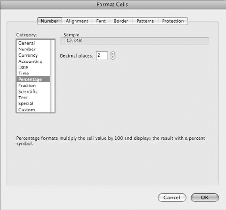
It is often convenient to display fractional values as a percentage. The Percentage data type makes this extremely easy to do. Simply select the Percentage type, as shown in Figure 14.7. The only other option available is the number of decimal places to use.
The Percentage data type takes the value entered in the cell and multiplies it by 100 for display, along with a percent sign (%). For example, the value 0.50 is displayed as 50%, and 2.0 is displayed as 200%.
Understanding Date Systems
Excel dates and times are represented internally as numeric decimal values, with the whole number portion to the left of the decimal representing the date and the decimal portion representing the time. Unfortunately, a long-standing incompatibility between Mac and Windows versions of Excel has caused some problems over the years. Excel on the Mac traditionally uses January 2, 1904, as the basis for its date values. The date portion simply counts the number of days since then. For example, January 1, 2009, is represented internally by the value 38352. Excel for Windows, however, uses January 1, 1900, as the basis for its dates.
This used to cause major headaches when sharing workbooks between Windows and Macs. Fortunately, this distinction is now largely academic, because Excel allows you to set the base date system to use for a workbook. Although Excel 2007 for Windows still uses 1900 and Excel 2008 for the Mac still uses 1904, an attribute is now saved with the workbook to indicate which system is in use, and it is recognized by either version. You can change the date system in use by choosing Excel

You can choose a base date system in the Calculation preferences under Workbook options.

With the Fraction data type, you can choose to display decimal data as the nearest fraction, with a whole number portion and the part after the decimal shown as a numerator/denominator fraction. Select the Fraction data type, and choose one of the fractional values shown in Figure 14.8. If the number cannot be represented entirely by the chosen value, it is rounded for display; the underlying value is never changed.
Tip
Some of the fraction types can be most useful for measurements, because portions of an inch are traditionally given in values of half, quarter, eighth, or sixteenth of an inch.

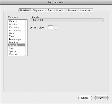
Scientists and engineers often work with very large or very small numbers, and the number of digits can become unwieldy and hard to see at a glance. With such numbers, the ultimate precision of the value is not as important, so E notation was developed to represent these values in a small amount of space.
With E notation, the decimal point is moved to a more convenient location for display, and the number of places it is moved is displayed after the letter E, along with a sign indicating the direction the decimal point moves. For very large numbers, the decimal point is moved to the left, and the E value is shown with a plus sign. For very small numbers, the decimal point is moved to the right, and the E value is shown with a negative sign. Table 14.1 shows some examples of E notation. Figure 14.9 shows the Scientific formatting options.
These number formatting options are nice, but sometimes you just want a cell to display data exactly the way you enter it. The Text formatting option, which is the default for any data that Excel can't determine how to apply another data type to, can be used to force all values to be displayed as entered, with no formatting changes. Figure 14.10 shows the Text formatting option.
Excel supports some formatting options that just don't fit anywhere else or merit their own category, so they've been tossed into the Special formatting category. These options, shown in Figure 14.11, include Zip code (and Zip +4), phone numbers, and social security numbers. These options are all U.S. formats.


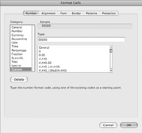
You've looked through all the provided formats and you can't find one that formats numbers (or dates) exactly the way that you like. Fear not, because Excel gives you the Custom formatting option so you can roll your own number formats. With the Custom type, shown in Figure 14.12, you can choose one of the provided basic types as a starting point and modify it to fit exactly the way you want. The Custom options are quite flexible; in fact, they are used to define all the existing formatting types behind the scenes.
Tip
You can see how the predefined formats are defined by selecting them and then switching to the Custom category.
The syntax for describing a custom format is a bit arcane, so it's helpful to see a table with the options and examples. Table 14.2 gives a list of codes and what they do. Table 14.3 lists date and time codes.
Table 14.2. Custom Number and Text Format Codes
Number and Text Code | Format |
|---|---|
General | General number. |
0 | Single-digit placeholder. Extra zeroes in a format indicate that numbers should be padded with zeros to fit if necessary. |
# | Single-digit placeholder, but with no zero padding. |
? | Single-digit placeholder, which leaves space for zero padding but does not display them. |
. | Decimal indicator. |
% | Displays as percentage. |
, | Thousands separator. |
E+, E-, e+, or e- | Uses scientific (E) notation. |
@ | Displays as text. |
+ - $ / ( ) : space | Displays characters directly in the format. |
character | Displays the character that follows the backslash. For example, ! displays an exclamation point. |
"text" | Displays the text inside the quotes. |
* | Repeats the next character in the format to fill in a custom width. |
_ (underscore character) | Skips the width of the following character. This can be used to line up one format with another when one displays a character and the other does not. |
[BLACK], [BLUE], [CYAN], [GREEN], [MAGENTA], [RED], [WHITE], [YELLOW], [COLOR n] | Displays the characters that follow in this color. The n value refers a value from 1 to 56, indicating one of the values of the Excel color palette. |
Table 14.3. Custom Date and Time Format Codes
Date and Time Codes | Format |
|---|---|
m | Numeric month without leading zero (1-12) |
mm | Numeric month with leading zero (01-12) |
mmm | Name of month, abbreviated (Jan-Dec) |
mmmm | Name of month, unabbreviated (January-December) |
d | Numeric day of the month, without leading zeros (1-31) |
dd | Numeric day of the month, with leading zeros (01-31) |
ddd | Day of the week, abbreviated (Sun-Sat) |
dddd | Day of the week, unabbreviated (Sunday-Saturday) |
yy | Two-digit year (for example, 09) |
yyyy | Four-digit year (2009) |
h | Hours as a numeric value, without leading zeros (0-23) |
hh | Hours as a numeric value, with leading zeros (00-23) |
m | Minutes as a numeric value, without leading zeros (0-59) |
mm | Minutes as a numeric value, with leading zeros (00-59) |
s | Seconds as a numeric value, without leading zeros (0-59) |
ss | Seconds as a numeric value, with leading zeros (00-59) |
AM/PM am/pm | Use a 12-hour clock |
Each custom format can have up to four sections, separated by a semicolon (;). These sections, from left to right, set formatting for Positive numbers, Negative numbers, Zero values, and Text values. You do not need to use all four sections; if you use one, it is used for all formatting. With two sections, the first is used for positive and zero values, and the second for negative numbers. Formats can be quite complex overall. Table 14.4 shows some examples that you might find useful.
Table 14.4. Custom Format Examples
Code | Format |
|---|---|
dd/mm/yyyy | Date in day/month/year format, with leading zeros and a four-digit year. Example: 29/03/2009 |
mmmm d, yyyy h:mm AM/PM | Long format date and time. Example: March 29, 2009 3:29 PM |
(000) 000-0000 | Displays as phone number. Example: (555) 123-4567 |
@*. | Text format, but pads the empty space in the cell with a period. Example: John.......... |
_($* #,##0.00_);_($* (#,##0.00);_($* "-"??_);_(@_) | The standard accounting format: three sections, describing positive, negative, and zero values |
Tip
Because Excel 2008 provides so many existing formats, you can use them to understand how custom formats work. Select an existing format, and then click the Custom category. The custom format displayed defines the last format you selected.
The second tab on the Format Cells dialog box—Alignment, shown in Figure 14.13—can be used to change the way text is displayed in a cell. You can change the horizontal and vertical alignment and set text wrapping and shrinking, cell merging, and even the orientation of the text. As you can imagine, all these options can lead to some very funky-looking cells.
Setting the horizontal and vertical text alignment can make a difference in how data is displayed in cells with expanded heights or widths, or when a single cell contains lots of data. You can choose from two alignment options: horizontal and vertical.
The default horizontal alignment, General, lets Excel try to determine the best way to display data. General alignment displays text aligned to the left and numbers aligned to the right. You can override this setting to have data conform to the alignment of your choice. You have these options:
General: Uses the default alignment that Excel assigns: text aligned to the left, numbers to the right.
Left (indent): Aligns to the left, with an optional indentation value that you can choose in the Indent box to the right of the alignment drop-down list.
Center: Centers data in the cell.
Right: Aligns data to the right of the cell.
Fill: Repeats data to fill up empty space in the cell.
Justify: Spaces text in a paragraph, with the exception of the last line, to fill the cell from left to right.
Center across selection: If multiple cells are selected, this option can be used to center the text based on the width of the selected columns. This is useful for centering titles over multiple columns, for example.
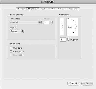
When text is too large to fit into a cell, Excel needs to know how to display it. By default with no text control, the data is displayed overlapping the cell next to it. This can be confusing and messy. Figure 14.14 shows some examples of text alignment formatting. These are your options:
Wrap text: Text wraps to additional lines if is too large to fit on a single line.
Shrink to fit: This reduces the size of the text in a cell so it all fits in the size of the cell.
Merge cells: If multiple cells are selected, they are merged together so more space is available for the other formatting options.

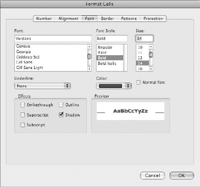
On the Font tab of the Format Cells dialog box, shown in Figure 14.15, you can choose from a myriad of text formatting items, including the font style and size, text color, and various effects. Each of these items can apply to an entire cell or to a subset of text in a cell. To apply it to a portion of the text in the cell, you must double-click the cell to get into Edit mode and then select the text you want to change.
As you make changes to the font settings, the Preview window shows you how these settings will make your text look.
The most important choice on this tab is the font to use. The right font can make the difference between readable text in a worksheet and a frustrating experience. Choose a font from the Font list. If you know the name of the font you want to use, you can type it into the Font box directly. The list scrolls as you type so you can quickly locate the correct font.
After you've chosen a font, you need to choose a style for it. Your options are Regular (no style), Italic, Bold, or Bold Italic.
Finally, choose a size for the font. Most fonts allow from 6 to 72 points in size. If a value you want to use is not listed, you can enter it directly in the Size box.
Choosing a font is simply the first step. You can apply additional formatting attributes to your data as well. These include various text effects as well as underline styles that are unique to Excel.
Excel gives you several underline styles, with two that are useful for worksheets oriented toward accounting:
None: Text is displayed without being underlined.
Single: Text is displayed with a single line under it.
Double: Text is displayed with two underlines. The second line is above the line used for the single underline. The spacing of the lines is not affected by the font size.
Single Accounting: Text is displayed slightly higher with more space between the font and the underline.
Double Accounting: In this double underline setting, the second line is below the one used for single accounting.
With effects, you can add more attributes to your data to present it in a special way. Effects can be applied alone or together, and each can be set individually. (Subscript and Superscript are exceptions; only one of those effects can be applied at a time.) These are your options:
Strikethrough: Text is displayed with a line through it.
Superscript: Text is displayed slightly smaller and above the main text. This is frequently used for exponents.
Subscript: The text is displayed slightly smaller and below the main text.
Outline: Only the outline of the text is displayed.
Shadow: A drop shadow is displayed below and to the right of the text. The color of the shadow is similar to the text color chosen for the cell, only lighter.
Nothing changes a worksheet from drab to interesting more than adding color. Colors can be used to make certain data stand out. For example, you could make cells in which you intend to have values manually entered appear in one color, cells that are locked appear in another color, and formulas in yet another color.
Excel offers a palette of 56 colors to choose from; simply use the Color drop-down list, shown in Figure 14.16, to make your choice. Keep in mind any background color that you may want to use. If you use a dark background, you should stick with lighter font colors. Darker colors are okay on white or lighter background colors. See "Setting a background pattern" for information on setting background color.
Note
Of special interest is the Automatic option. This option may seem to always make your text black, so you may wonder why they bother with this option. It is useful when you save a worksheet as an HTML page for viewing in a Web browser, because the browser takes the user's default color preference for both the text color and the fill color. Therefore, if you don't have any other color changes, you should consider leaving the default setting of Automatic in place out of consideration for people who may view your worksheets over the Web.
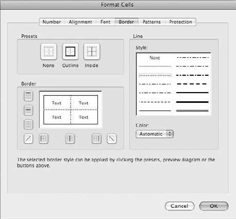
Another option for custom cell formatting is to use the border feature. Borders can be used to accentuate a cell, a range of cells, or a row or column. You can disable borders to give your worksheets a clean look. Most aspects of a cell's border presentation can be set independently of one another. You can turn each border on and off individually and even give each one a unique color if you like. Figure 14.17 shows the Format Cells dialog box's Border tab.

To change cell borders, follow these steps:
Select a cell or range of cells, and open the Format Cells dialog box as described earlier.
Choose a line style, if desired. The default is a solid line, but other options are available, including thicker lines, a double line, various broken and dashed lines, as well as no style at all.
Choose a color for the border, if desired.
Click one of the preset buttons to apply borders:
If you want to enable or disable an individual border, use one of the individual border buttons located in the Border section. You also can toggle borders on and off by clicking them directly in the preview window.
If you want to give some borders a different style or color, repeat Steps 2 through 5 for those borders. One popular option is to make outline borders thicker and darker, but leave inside borders lighter or dashed.
Click OK to apply the border change.
Note
Cells share borders with other cells, and a conflict can occur as to which border setting is used. In general, the last border setting made overrides a previous one. For example, if you make the right border of a cell red and then the left border of the adjacent cell blue, the blue border is used.
The final step in customizing a cell's format is to set a background color or pattern. This is done on the Patterns tab of the Format Cells dialog box, shown in Figure 14.18.
Even though the tab is labeled Patterns, the most common option to set here is the solid background color of a cell. To do so, simply choose one of the 56 offered colors in the palette. The Sample window shows you a larger filled area of the color. Click OK to apply the new color.
If you like, you can set a pattern for the cell's background instead. The patterns you can choose from include a variety of horizontal, vertical, and diagonal lines, as well as some crosshatch patterns. You can use these patterns to emphasize certain cells. To set a pattern, choose one from the drop-down menu shown in Figure 14.19. Use the same menu again to choose a color to use for the pattern.
Tip
If you want cell text to be readable against the pattern, use a lighter pattern color to go with darker cell colors.


So far, we've been focusing on the Format Cells dialog box, and with good reason: It's the place to go for all the formatting options available to you. You can use other tools to set formatting, one of which is the Formatting toolbar, shown in Figure 14.20. If the Formatting toolbar is not visible, you can enable it by choosing View
Figure 14.20. The Formatting toolbar presents a handy way to apply the most commonly used formatting options.
Table 14.5 shows the options available on the Formatting toolbar.
Table 14.5. Custom Format Examples
Icon | Function |
|---|---|
Lets you choose a font name from the drop-down menu, along with the font size. | |
Sets selected text Bold. | |
Sets selected text as Italics. | |
Underlines the selected text. Only the standard single line underline is available here. | |
Aligns text to the left. | |
Centers text in the cell. | |
Aligns text to the right. | |
Merges selected cells, and centers text within the combined cell. | |
Applies the Accounting data format. | |
Applies the Percentage data format. | |
Applies the standard numeric format, with two decimal places and the thousands separator. | |
Decreases the number of decimal places displayed by one. | |
Decreases indent. | |
Increases indent. | |
Lets you choose a border style from the drop-down menu. | |
Lets you choose a text color. |
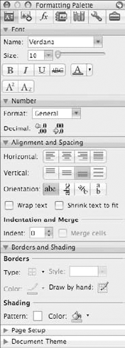
The Formatting Palette is part of the Toolbox floating palette, as shown in Figure 14.21. The Formatting Palette doesn't give you as many formatting options as the Format Cells dialog box, but it does give you more to work with than the Formatting toolbar. It also puts all the controls within a single click without forcing you to try to remember which tab contains a particular setting. An additional advantage is that changes are applied in real time to your worksheets, so you don't have to make all your formatting choices and click OK to see them; you can decide whether a particular format works as you're making changes. If the Formatting Palette is not visible, you can activate it by choosing View
The Formatting Palette offers some unique controls for formatting cells and is organized in categories that can be expanded or closed, depending on which ones you want visible. The following categories are available:
Font: Here you can set all the usual font selection options, including typeface, size, color, and effects. One unique option available here is the slider control that can be used to select a font size.
Number: This category can be used to set basic number formatting. While all the number format data types are available from this list, only one of each type is available. If it's not exactly what you want, you have to use the Format Cells dialog box. You also can increase or decrease the number of decimal points visible using buttons located here.
Alignment and Spacing: You can select the most common text alignment options, as well as orientation, text wrapping, and cell merging in this category.
Borders and Shading: Choose a border style and color, or set the background color of a cell in this category. For added convenience, you can use the Draw by Hand button to change borders directly on the worksheet.
Page Setup: This category can be used to configure your worksheets for printing. These options are discussed in detail in Chapter 18.
Document Theme: This category lets you choose a document theme, which is discussed later in this chapter.
So you've spent hours creating the perfect formatting, and you're very happy with how it looks. The only problem is that you now want to apply the formatting to other worksheets or workbooks. Fortunately, you don't need to redo each individual format setting from scratch: Excel gives you the ability to copy formatting from one cell and paste it directly into another.
The easiest way to copy formatting is to use the Format Painter icon on the Standard toolbar. Follow these steps to copy formatting from a cell or range of cells to another:
Select the cell or range of cells that contain the formatting that you want to copy.

Select the cell or range of cells to which you want to copy formatting.
The formatting is automatically applied.
Repeat Steps 2 and 3 to apply the formatting to additional cells, as shown in Figure 14.22.
Another way to copy formatting is to use the Paste Special feature. By default, all formatting is copied when you copy and paste a cell, but the Paste Special dialog box lets you be a little more selective. Here's how:
Select the cell or range of cells that contain the formatting that you want to copy.
Copy them to the clipboard using one of the Copy commands—for example, by choosing Edit
Copy.Select the cells to which you want to copy the formatting.
Choose Edit
Paste Special to open the Paste Special dialog box.Select the formatting options that you want to copy. You can choose just to copy formats or just copy number formats and values, along with some other options shown in Figure 14.23.

Even though you want pretty worksheets and all this formatting stuff makes sense, it still seems too much like work to get a professional-looking result. What you really want is a feature that automatically formats an entire worksheet to save you some time. Excel's AutoFormat feature can do just that. AutoFormat gives you 17 options that immediately make your worksheets look like a pro did them, even if this is your first day using the program.
AutoFormat is really designed around table type data. It applies font, color, number, and border formats to the range of cells you select. Unfortunately, you have to enter the data and text yourself. To use AutoFormat, follow these steps:
Select the cell range to which you want to apply the formatting.
Choose Format
AutoFormat. The AutoFormat dialog opens, as shown in Figure 14.24.Choose a format style that matches your desired look and the purpose of your workbook.
Click the Options button to reveal a set of check boxes that let you choose a subset of the format options to apply. Check and uncheck these as desired.
Click OK to apply the formatting.

After you have applied AutoFormat formatting, you are free to make further changes using any of the methods described in this chapter, using the Format Cells dialog box, the Formatting toolbar, or the Formatting Palette.
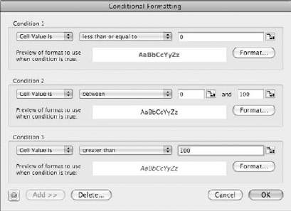
Conditional formatting is a feature of Excel that lets you set rules for how cell formatting will look. Each cell can have up to three rules; if the conditions of a rule are met, the formatting is applied. You can use conditional formatting to emphasize values that are of interest, such as when a value is outside of a desired range—say, when your budget goes negative. To define conditional formatting for a cell, follow these steps:
Select the cell or range of cells to which you want to apply conditional formatting.
Choose Format
Conditional Formatting. This opens the Conditional Formatting dialog box, shown in Figure 14.25.Under Condition 1, choose whether you want the condition to be triggered from a value or from the result of a formula. The formula option is often more useful, because cells with formulas are more likely to have changed data. However, the value option gives you flexibility in choosing operators. These are your choices:
Cell Value Is: If you choose this option, select a conditional phrase from the next pop-up menu, and then enter a value to compare it to in the last field.
Formula Is: Enter a formula that evaluates to either TRUE or FALSE.
Click Format, and choose the formatting options for font, border, and patterns. Conditional formatting has a limited subset of formatting options available. For example, you can't choose a different font or font size, but you can choose a font style (bold, italics, or underline), underline and strikethrough effects, and text color. Figure 14.26 shows the Font tab of the conditional formatting version of the Format Cells dialog box.
Click OK to add the format.
To add additional conditions, click the Add button in the Conditional Formatting dialog box. You can have up to three conditions; if none of them evaluates to TRUE, the normal cell formatting applies. If more than one condition evaluates to TRUE, the first one that does so applies.

You may find yourself using the same formatting options over and over again, and it can be painful and time consuming to have to redo them every time. Fortunately, Excel gives you the ability to save formatting options so that they can be reused again later. Your styles are saved along with the workbook, and it's easy to refer to them again in order to apply that style (or a portion of it) to additional cells. You can even copy a style to another open workbook.
Tip
Excel remembers which styles have been applied to a cell. If you make modifications to the style, the formatting changes are automatically applied to all cells that use the style. This can make it easy to make sweeping formatting changes to a workbook simply by changing a couple styles.
You can base a style on an existing format, create one from scratch, or do some combination of the two. Follow these steps to create or modify a style:
Select the cell or cells that contain the formatting you want to use as the basis for the style.
Choose Format
Style to open the Style dialog box, shown in Figure 14.27.If you want to make changes to the formatting or are creating formatting from scratch, click the Modify button. Then make formatting changes in the Format Cells dialog box as described earlier in this chapter.
Uncheck any formatting styles that you don't want to include in the style. You can include or exclude number, alignment, font, border, pattern, and protection styles.
Enter a name for the style in the Style Name box.
Click Add to create the new style.
Click OK to apply any changes to the style to the selected cells.

After you create a style, you can easily apply it to other cells. You also can choose to apply one of the standard styles that have been provided. Follow these steps to apply a style:
Select the cell or cells to which you want to apply the style.
Choose Format
Style to open the Style dialog box.Choose a style from the Style Name menu.
Uncheck the style attributes you don't want to apply, if any.
Click OK to apply the style.
After you are happy with a style, you likely will want to use it all the time, in all your workbooks. Excel makes it easy to merge styles from one workbook into another so you can do just that. Follow these steps to merge styles from one workbook into another:
Open the workbook containing the styles you want to copy.
Open or create the new workbook.
In the new workbook, choose Format
Style to open the Style dialog box.Click Merge.
Choose the source workbook in the Merge Styles dialog box, shown in Figure 14.28.
Click OK to apply the styles.

Note
When you merge styles from another workbook, there is a chance that the names of those styles will conflict with styles in the destination workbook. If this occurs, Excel gives you a warning and asks if you still want to merge the styles. If you say yes, the existing styles using those names are replaced by the new ones and any cells that make use of those styles have formatting changed to match.
While you were learning about the Formatting Palette, you may have noticed that we skipped over the Document Theme pane. Document themes are combinations of color schemes and fonts that work well together. Excel can use the same themes as Word and PowerPoint, which makes it very easy to coordinate your presentations and supporting documents so they present a consistent image. However, themes have a significant limitation in Excel; they don't apply to worksheets directly, only to charts, SmartArt graphics, shapes, and pictures. If you make use of any of those features, however, use themes to provide consistency with Word and PowerPoint documents.
To apply a theme to your workbook, do the following:
Open the Formatting Palette, and expand the Document Themes section if it's collapsed. This pane is shown in Figure 14.29.
Choose a theme from the list, or browse for a custom one that you created in PowerPoint.
If you prefer, you can choose a color combination and font individually.

Figure 14.29. Document themes can be applied to SmartArt, charts, shapes, and pictures to provide a consistent look with Word and PowerPoint documents.
Office provides 50 themes, but you are not limited to these. You can create your own themes by modifying the colors and fonts to suit your needs and then clicking Save Theme from the Document Theme pane.
Formatting can make a plain, mundane worksheet special—if not exciting, at least a little more pleasant to look at and work with. Excel 2008 provides an array of formatting options. You learned how to apply number formatting to cell values to allow them to contain general formatting, numbers, currency, accounting, date and time values, percentages, fractions, and scientific values. If that's not enough, you learned how to create custom formats as well.
You also learned how to apply formatting to the text in your worksheets, giving you the ability to change fonts, alignments, line wrap functionality, and even text orientation. You learned how to set borders and color information for cells.
This chapter showed you how to apply formatting using the Format Cells dialog box, the Formatting toolbar, and the Formatting Palette. You learned how to use AutoFormat and Conditional Formatting and how to create and apply styles and document themes.
In the next chapter, you learn how to work with formulas and functions to perform a wide variety of computational tasks.