IN THIS CHAPTER
Checking your spelling
Previewing workbooks
Printing workbooks
Collaborating with a team
Tracking and reviewing changes
Your presentation is in two days, and you've got PowerPoint slides ready to go. Now all you need to do is to be able to present the numbers that you've crunched in Excel, and you're all set. What you need to do is print your worksheets so the content is both clear and visually appealing. While the slides are what people see at the presentation, the Excel printouts are what they take back with them to study.
Or maybe you're a project manager tracking team progress over the course of a development cycle. You've been tracking everybody's assigned tasks and estimates in an Excel spreadsheet, and you need to print them so everyone can discuss them at the weekly meeting.
What these examples show is that no matter how productive we've become in the modern computer-enabled office, we still need to print stuff. Sometimes, it's just easier to sit with a printout and a highlighter, making notes.
This chapter explores Excel's print capabilities and shows you how to get the most from hard copies of your worksheets. However, if you're striving for electronic sharing, we show you how your team can work together using Excel's collaboration features, too.
At first glance, it might not seem that Excel workbooks would need extensive proofreading, but if you think about it, Excel workbooks contain text information almost as often as they have numbers. Field names, headings, instructions, and lists are just as deserving of proofreading as a newsletter that you are creating in Word. Fortunately, Microsoft agrees, so it provides many of the same proofreading capabilities in Excel that it does throughout the Office suite.
Although Excel doesn't include some of the more advanced features that Word offers in this area, such as automatically correcting spelling as you type or a grammar checker, it does include some other autocorrect options, a spell-checker that uses the same dictionary that other Office applications use, and the ability to access the dictionary and thesaurus references.
While Excel doesn't include Word's ability to autocorrect spelling mistakes as you type, it does include the same manual spell-checking capabilities. Before you print or share a workbook, run it through the spell-checker to clean up any problems. To do this, choose Tools
When Excel encounters an error, it displays the word in the dialog box, with suggested spellings listed below the error. To change the word to one of the suggestions, click the correct spelling and press Change. To change all occurrences of that misspelling throughout your document, choose Change All. If it isn't an error at all, such as with technical terms, names, or other uncommon words, you can choose either Ignore (for that specific incidence) or Ignore All (to ignore that word throughout the workbook). If it's a word that you expect to use often, click Add to append it to the default custom dictionary.
If none of these options solves your problem, you can correct the spelling error directly in the dialog box. Finally, if you commonly make the same typo, click the AutoCorrect button to add the typo and correctly spelled word to the AutoCorrect list.

A handy feature that Excel includes in its Toolbox is the ability to look up words in a variety of reference works, including a dictionary, a thesaurus, the Encarta online encyclopedia, or even on the Web. You can even do translations or look up foreign language words. Choose View
In Chapter 6, you learned about using the AutoCorrect feature in Word. Well, Excel has AutoCorrect capabilities of its own, even if they are a bit more limited. Choose Excel


Figure 18.3. Enable AutoCorrect options in the Excel Preferences to help correct errors as they are typed.
With AutoCorrect, you can have Excel automatically catch some common mistakes as you are typing, such as extra or missed capitalization and capitalization of the names of days of the week. It also provides a list of words and phrase that it automatically corrects as you type. This list includes some words with commonly transposed letters and misspellings, as well as some automatic translation of such things as copyright or trademark symbols. You can add or remove items from this list as you see fit or add them from the spell-checker.
Your workbook is completed, and you've proofread it and corrected spelling errors, so now it's time to print. You might want to print the entire workbook or just a single sheet or a portion of a sheet. Some options for formatting workbooks only apply when printing or in Page Layout mode, such as headings and footers. In this section, you learn how to define print areas, preview your workbooks before you print them, and configure the various print options for Excel.
Sometimes you don't want to print an entire workbook or worksheet, but only a portion of it. For example, you might have a section of a sheet that includes lots of data, and another section with formulas and formatting for display, for example. You can define a print area to include only the formatted part, but leave the raw data alone. To define a print area, select the range of cells that you want to include and choose File
If you want to print multiple areas of the worksheet, you can choose File
Before you print, you can configure quite a few options for your workbook to display in the best way possible. These options include page orientation, scaling, margins, headers and footers, and more. Choose File

Figure 18.4. When you define a print area, it is marked with a dashed line around it, and printing is restricted to print area content.
Click the Page tab to set options that for printing the page as a whole. They include the following:
Orientation: You can choose between Portrait and Landscape orientation. Worksheets often have a layout that is wider than it is tall, so the Landscape option can come in quite handy.
Scaling: You can scale the worksheet to a percentage of its normal size, or you can have it automatically scaled to fit into a certain number of pages or even a single page. Scaling can be useful when your worksheets are just too large to fit on a single page. Rather than have a few columns print on another page, scale the whole printout to fit. Use the Print Preview feature to verify that your scaling settings are just the way you like them.
First page number: You can leave this set to Auto to have Excel automatically determine a page number to start with when printing page numbers. You can specify 1 or some other number to customize the page numbering.
Print Quality: Choose High or one of the specific print quality settings.

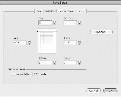
Click the Margins tab, shown in Figure 18.6, to make changes to the margins of your printouts. You can set the width of the left, right, top, and bottom margins, as well as the margins for the header and footer. Units are inches, centimeters, or millimeters, depending on the units you have defined in the General panel of the Preferences dialog box.
You can configure centering options on this tab as well. Check the Horizontally or Vertically boxes to control centering. This is particularly useful when printing a small worksheet or data range.
Click the Header/Footers tab, shown in Figure 18.7, to add or edit headers and footers. You can use headers and footers to customize the information to the top and bottom of every printed page, including page numbering, company information, or workbook filename. As their names imply, headers appear at the top of the page, while footers appear at the bottom.

Figure 18.7. The Header/Footer tab lets you customize the information printed at the top and bottom of each page.
From this tab, you can manually enter header and footer details, such as the title of your workbook, and this information then appears at the top (or bottom) of every page. Headers and footers have three sections each: left, center, and right. Each section can be customized individually to give you exactly the information you want.
The easiest way to add a header or footer is to choose one from the list of headers and footers that Excel already knows about. These are a mix of previously used headers and footers, filename information, and some standard ones. Choose one from the pop-up menu for both the header and footer.
If one of the provided headers or footers isn't quite what you want, you can click the Customize Header (or Customize Footer) button to create your own. These buttons open the Header and Footer dialog boxes, shown in Figure 18.8. Note that these dialog boxes are identical in terms of features.
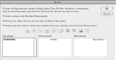
In the Header (or Footer) dialog box, you can enter information for the left, center, and right sections. Several buttons allow you to enter some pre-formed bits of text and auto-generated text:
Format Text: This lets you customize the font and effects used for the text. You can set it for the entire box or just for a selected portion of the text.
Insert Page Number: This is the most common header or footer content. You also can type the word "Page" into the header/footer, add a space, and insert the page number.
Insert Number of Pages: This field tallies the number of pages in the document and prints that total in the header or footer. You can use this to format a "Page X of Y" type header. To do this, type "Page" and add a space, click the Insert Page Number button, type "of" and a space, and then click the Insert Number of Pages button.
Insert Date: This inserts a date field into the header or footer. This field is automatically updated every time you modify the document, so when you print the document it reflects the date of printing.
Insert Time: As with the date option, this field automatically updates with the current time when you modify the document.
Insert File Path: This inserts the path to the workbook into the header or footer. If you organize your documents in hierarchical folders or on a network share, this can help you remember where the original workbook lives.
Insert File Name: This inserts the filename of the current workbook.
Insert Sheet Name: This can be used to insert the name of the worksheet. This can be useful if you use custom worksheet names, and why wouldn't you?
Insert Picture: This can be used to insert a picture such a company logo. The picture can be in any of the supported Office picture file formats.
Format Picture: This button becomes active when you've added a picture. It opens the Format Picture dialog box, where you can scale the picture and enter cropping settings. You can make some color settings including black and white, grayscale, watermark, or automatic. You also can adjust brightness and contrast.
To view the header and footer areas in your document, change to Page Layout view by choosing View
You can go directly to the Headers/Footers tab of the Page Setup dialog box by choosing View
The final tab of the Page Setup dialog box is the Sheet tab, shown in Figure 18.9. Click the Sheet tab to configure information relevant to printing worksheets, including titles, page order, and other formatting settings.

Figure 18.9. The Sheet tab of the Page Setup dialog box is used to control how worksheets are printed.
The following settings are available:
Print titles: You can set aside some number of rows and columns to use as titles on each page. This option is useful if you are printing columns of data that have title and header information in the first rows or wide rows with headers on the left. Note that you can't enter a number here, but rather you can enter a row reference such as 1:3 to repeat the first three rows or A:A to use the leftmost column. You can choose a range of cells by clicking the collapse button and selecting them directly from the sheet.
Print area: You can enter or select a range of cells to use as a print area. This has the same effect of defining a print area as the File

Gridlines: Checking this option causes gridlines to be included in the printout. They are not included by default.
Black and white: Check this option to force the printout to be in black and white even on a color printer. With some printers, you can save color ink with this setting.
Draft quality: Check this to force the printout to be in the lower-quality draft mode to speed up printing.
Row and column headings: Check this box to have Excel's row and column identifiers added to printouts.
Comments: Choose a setting for printing comments. Choices are None, at the end of the sheet, or as displayed on the sheet.
Page order: Choose to print down, then over or Over, then down. These options control the order in which pages are printed when your workbooks are more than one sheet wide and more than one sheet long.
Each tab of the Page Setup dialog box has an Options button. Click this button to open another Page Setup dialog box similar to the one available in Word and shown in Figure 18.10. In this dialog box, you can set some additional page settings. You can choose paper size, a printer to format for, and orientation and scaling settings (which are identical to settings described earlier). You also can choose to save these settings as the default using the Settings selection.


Many options are available in the Print dialog box, including these more common ones:
Printer: If you have multiple printers on your system, you can select one here. You also can use this as a jumping off point to configure a new printer.
Presets: You can save settings that you commonly use by choosing Save As from this pop-up menu and entering a name. When you wish to reuse those settings, you can choose it by name from this menu.
Print Options: This pop-up menu lets you change the view of the Print dialog box to allow for advanced settings. The views available in this menu may vary depending on your printer and driver, but may include some of the following: Copies & Pages (the default), Layout, Color Matching, Paper Handling, Paper Feed, Cover Page, Scheduler, Quality & Media, Color Options, Special Effects, and Duplex Printing and Margin. That's lots of options and more than we have room to cover in this book, but information on these settings is available in the Excel Help file. The Summary view is the last option on the menu and allows you to review all of the settings.
Copies: Choose the number of copies to print. Check the Collated box to ensure that an entire copy of the document prints before the next one is started. Uncheck this box to cause each copy of an individual page to be printed before the next page.
Pages: Choose the pages to include in the printout—either All or a range. You can use the Quick Preview view to get an idea about what each page would include.
Print What: You can choose to print the selected region of the active sheet, the entire active sheet, or the entire workbook.
Scaling: You can choose a scaling option here to force the document to fit within a certain number of pages wide and tall.
Show Quick Preview: Check this box to enable the small quick preview window. You can use the arrow keys to move from page to page.
Page Setup: This opens the Page Setup dialog box.
Preview: This lets you preview the document in the OS X Preview application.
PDF: This menu includes options for saving the formatted document as a PDF or PostScript file, mailing it, or faxing it.
Supplies: This launches a Web browser to navigate to a site where you can purchase printer supplies such as toner or ink cartridges.
Print: This prints the document using the entered settings.
With Excel 2008, Microsoft decided to drop Excel's built-in preview functionality in favor of the OS X Preview application, shown in Figure 18.12. And no wonder: Preview gives you a great deal of flexibility in working with the formatted document. In Preview, you can choose individual pages from the sidebar on the right or use the scrollbar to scroll through your pages. You also can perform all the other functions that Preview can do—save the printout in PDF or as an image, delete individual pages that you don't want to include, and even mark up text and add annotations. You also can print directly from Preview application. To preview, click the Preview button from the Print dialog box.

When you work in a team environment, several people often need to work with the same documents. This can be true especially for workbooks, which are often used as continually updating "working documents." Excel sees lots of use because of its ability to make lists, track schedules and estimates, and work with oft-updated financial and other numeric data. Because Excel is included in every version of the Microsoft Office suite on both the Mac and Windows, a huge number of people can make use of it.
One of Excel's unique features in the Office suite is its ability to share workbooks. At first glance, this may not seem particularly useful; after all, any document can be "shared" if it sits on a network file server and multiple people have access to it. Excel, however, goes beyond this by including features that allow users to make changes to worksheets at the same time. That is to say, when you enable workbook sharing, Excel keeps track of who has the worksheet open, and who has saved it most recently. When you attempt to save over somebody else's changes, Excel merges their changes into your workbook first. Best of all, this feature is compatible with other versions of Excel such as Excel 2003 and Excel 2007 on Windows, so for once you don't have to forgo a feature if you are the lone Mac user in the office. Sound useful? Read on.
You can use workbook sharing automatically with any workbook; you just have to enable it first. This couldn't be simpler though; simply choose Tools

Figure 18.13. The Share Workbook dialog box is used to control how and who can access a shared book.
On the Editing tab, check the Allow changes by more than one user at the same time option to enable sharing. That's it! Your workbook can now be shared, after you click the OK button, that is.
On this tab, you also can see a list of people who have the worksheet open. You can also remove them from this list if necessary. This is sometimes necessary if the person who opened the workbook doesn't close it before disconnecting from a network share or powering off his computer. When this happens, Excel doesn't get a chance to remove them from the list before closing.
You can set some additional options on the Advanced tab, shown in Figure 18.14. These are as follows:
Track changes: You can keep track of the change history for a period of time. The default is 30 days. The change history can be viewed either directly in the document or on a history worksheet. We cover more on this feature later.
Update changes: Choose how to apply updates that other people may have saved. The default is to update them whenever the file is saved, but you can choose a time interval to perform updates, and choose whether this interval should update the saved document with your changes or just merge any saved changes into your open document.
Conflicting changes between users: If another user changes information in a workbook—such as a cell data value or formula—and you also change the same value, you will have a conflict when the changes are updated. This setting controls how conflicts are handled. You can choose to have the user prompted to choose which change to use (highly recommended) or just have the most recent version of the changes take precedence.
Include in personal view: These settings allow individual users' print and filter settings to be saved with the workbook. This can be useful if users make use of different printers.

When two users are editing the same workbook frequently, conflicts can occur if they update the same data in the document at the same time. When this occurs, and you configured the Workbook Share settings to prompt the user to resolve conflicting changes, the Resolve Conflicts dialog box, shown in Figure 18.15, is launched. In this dialog box, you can see how each user changed the workbook, with your changes on the top and the saved changes on the bottom. You can select individual items and click the Accept Mine button to have your changes take effect or Accept Other to keep the saved version. If there are many changes, you can use the Accept All Mine or the Accept All Others buttons to choose either all your changes or all the saved changes. You can click Cancel here if you don't want to risk making any changes, in which case your changes are not saved.

Although Excel can automatically merge changes when you save on top of a changed document, sometimes you don't have the luxury of working that way. Sometimes you or your teammates need to take work home or otherwise work remotely with files, and you may not be connected to the network. Sometimes you mail a copy of a document for review to many people, and you want the ability to merge all their changes into your original workbook. This is easy to do with the Merge feature. To manually merge changes from another workbook, simply save it to a location on your hard drive or on a network share, and choose Tools
When multiple users are making changes to a workbook, it can be nice to track the changes so you can decide to accept or reject them, or at least to see what those changes were. The Track Changes feature in Excel can be used in both ways.
If you would like to see the changes that other users (and you) have made, choose Tools
You have these options in this dialog box:
Track Changes while editing: Check this option to enable change tracking while editing. This option is automatically enabled when workbook sharing is turned on, and vice versa.
Highlight which changes: You can choose to highlight changes made during a specific time period, for specific users, or in a portion of the workbook. The options are When, Who, and Where. Uncheck all the options to track all changes in the history:
When: Highlight changes made over a time period. Sub-options are Since you last saved, All, Not yet reviewed, and Since Date.
Who: Highlight changes made by Everyone, Everyone but you, or just you.
Where: If you are interested only in changes made in a specific region of the worksheet, choose a region to put in this box.
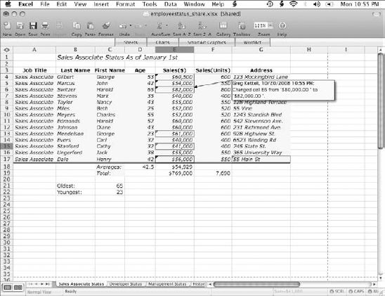
Highlight changes on screen: Check this option to have changes highlighted on the screen, shown in Figure 18.17. You can move the mouse pointer over a highlighted cell to see exactly what has changed in a pop-up window.
List changes on a new sheet: If checked, a special worksheet named History is created with a list of changes. This worksheet cannot be deleted or modified directly. The History worksheet is shown in Figure 18.18.

When tracking is enabled, you have the opportunity to accept or reject changes if you like. Choose Tools
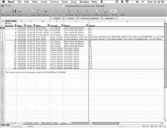
Figure 18.18. If you prefer to get a listing of changes made, you can have them appear on a separate worksheet.
In this dialog box, you can make the same three choices (When, Who, and Where) that are described earlier for the Highlight Changes dialog box. The choices act a little differently, however:
When: Highlight changes made over a time period. You can accept or reject changes Not yet reviewed and Since Date. Use the Not yet reviewed option if you want to get a chance to accept or reject all changes and keep up with it. If your document has lots of changes and you want to decide only on the most recent ones, choose Since date and adjust the date as appropriate.
Who: Accept or reject changes made by Everyone, Everyone but you, or just you. If you are the main reviewer of other people's changes, you might find the Everyone but you option preferable.
Where: If you are only interested in changes made in a specific region of the worksheet, choose a region to put in this box.
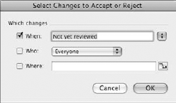
Leave all boxes unchecked if you want the opportunity to accept or reject all changes. After you've selected which changes to review, click OK. Excel then iterates over all the changes in the workbook. If it finds changes that haven't been accepted or rejected yet, the Accept or Reject Changes dialog box, shown in Figure 18.20, is opened.

Figure 18.19. Use the Select Changes to Accept or Reject dialog box to decide which changes you want to approve.
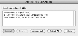
Figure 18.20. The Accept or Reject Changes dialog box iterates over unreviewed changes and gives you an opportunity to keep them or revert to the original setting.
In the Accept or Reject changes dialog box, you can choose to accept or reject an individual change, or accept or reject all remaining changes. When you accept them, the changes are applied to the worksheet. If you reject changes, they revert to the way they were before the change. You can stop at any time by clicking the Close button, and any remaining unreviewed changes are still available the next time you run the command.
If a particular item has been changed multiple times since the last time you reviewed changes, you have the opportunity to choose any of the change values, as shown in Figure 18.21. Click one of the changed values to select it, and click Accept. When you have finished reviewing all the changes, save the workbook to ensure that the next time you review it, you only need to see new changes.
Sometimes when you are reviewing a worksheet for somebody, all you really want to do is add comments to ask questions or point something out. Then, when you send it back to them or merge changes, they can use the Track Changes feature to scan through the comments and accept or reject them as they see fit. The Reviewing toolbar can make things easier for both the reviewer and the workbook author by letting you easily add comments, navigate from comment to comment, and show or hide comments. Choose View
The Reviewing toolbar has the following options:

Excel is a great tool to use in a team environment, whether you prefer to work with hard copy printouts or electronically. You can take advantage of Excel's advanced printing and previewing features to create printouts that show your work in the best light. You can print workbooks in whole or in part, and adjust, scale, and add headers and footers to identify the content. When you are ready to print, you can preview your work in the OS X Preview application, which lets you add annotations and markup to the document, delete any extraneous pages, or save the formatted output in a variety of formats, including PDF.
If collaborating with coworkers is more your thing, Excel's workbook-sharing feature makes it possible for several people to make changes to a workbook at once. Excel can track changes made by others and automatically merge them into your copy of the workbook when you save or at a specified interval. You can view the change history to see any changes that have been made in a specified amount of time, or even step through changes one by one to accept or reject them. Finally, the Reviewing toolbar can help you if you rely on having people add comments to a workbook as they review it. You can use this toolbar both to add and edit comments, but also to step from one to another, delete comments, or even mail the workbook directly to a reviewer (or from a reviewer back to you).