
23
Analysis of a Multiserver System of Queue-Dependent Channel Using Genetic Algorithm
Anupama1⋆ and Chandan Kumar2
1Department of Mathematics, Darbhanga College of Engineering, Darbhanga, Bihar, India
2Department of Mechanical Engineering, BIT Sindri, Jharkhand, India
Abstract
In the present work, a M/M/3 Queuing system with a Queue-dependent multi-server has been considered. Here, a number of failed machines form a queue and repairmen consider a service provider or service channel which starts its service when the queue length is N. We found a generating function for breakdown machines. Afterwards, some performance measures including idle time and busy time for the system have been evaluated. At last, cost is optimized using a genetic algorithm.
Keywords: M/M/3, repairmen, queue dependent server, genetic algorithm
23.1 Introduction
The concept of a multiserver queueing system with queue-dependent servers is not new. Hahn and Sivazlian, in 1990, developed the M/M/2 model with service stations [5]. Yadin and Naor, in 1963, invented the N policy concept for the single server system [9]. The (0, K, N, M) rule in a two server system used by Rhee and Sivazlian in 1990 helps to derive the working period distribution [12].
Natarajan studied a system for warm stand-bys in 1968 [13]. With one online unit and two standbys with failure and repair time exponentially distributed, this model assumes only one condition, namely that the system will fail if spares are not present for the breakdown machine. There is an analytical closed-form solution for the M/Ek/1 system [15]. The server system for standbys and 2 types of failure time distribution is also examined. Wang and Ke (2000) introduce a supplementary and recursive technique for developing a solutions to a single server queueing system working with the N policy [16]. The current system is that the line length determines the server value in the system. In the event that no machines fail in the system, all the fixers are temporarily inactive until the length of the line reaches a predetermined level, i.e., W, which is also a decision change. For this single server period, it will be activated instantly. Sometime later, if the line length in the system goes up to the aforementioned level, it says S, which is less than W and then the other available server will also run immediately. Similarly, if the failure machines in the system go up to a next level, say T, which is less than S, then all the servers will be activated immediately.
The objectives of this paper are:
- To achieve a sustainable distribution of waiting line opportunities
- Finding average count of failed machines
- To design the total cost of the model
- The genetic algorithm method is used to optimize costs
23.2 Description of the Model
The states for the model depicted by [i, n], i = 0, 1, 2, 3 represent that no repairman is working, one of the repairmen is working, two of the repairmen working, or three of the repairmen working, respectively. n Є [0, L] is the number of failed machines in the model.
23.3 Notations
ϸ[0, n] = Occurrence of n customers in the model where there are no operators, when n Є [0, W-1]
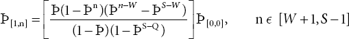
ϸ[1, n] = Occurrence of n customers in the model when one modifier works, when n Є [0, S-1]
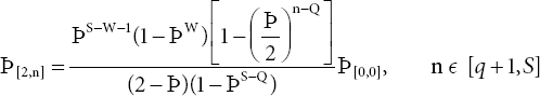
ϸ[2, n] = Occurrence of n customers in the model, where two moderators are working, when n Є [q + 1, T-1]
ϸ[3, n] = Probability of n customers in the system, where three moderators are working, when n Є [r + 1, L].
α = Average arrival rate
β = Average service level
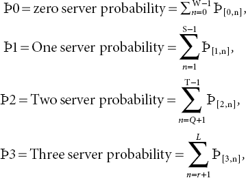
ϸ0 = Zero server probability in the system
ϸ1 = One server probability in the system
ϸ2 = Two server probability in the system
ϸ3 = Three server probability in the system
L0 = Line length of the system if all fixers are on vacation
L1 = Length of the line in the system where a single server is working in the system
L2 = Line length in the system where two modifiers are working in the system
L3 = Line length in the system where all three fixers work in the system
Ls = Line length in system
EI =Idle time expected value
E B1 = Busy time expected length during which any repairman is working on the system
E B2 = Busy time expected length during which any repairman is working on the system
E B3 = Expected length of busy time during which every repairman works on the system
E C = Busy time expected length
Ch = Cost of each failed machine during the unit available in the system
Cv1 = Cost savings per failed machine during each unit in the system when 1 mechanic is on vacation
Cv2 = Cost of handling per failed machine during each unit present in the system when 2 technicians are on vacation
Cv3 = Cost savings per failed machine during each unit present in the system when 3 technicians are on vacation
C01 = Holding cost of single technician functioning in the system during each unit time
C02 = Holding cost of 2 technicians functioning in the system during unit time
C03 = Holding cost of 3 technicians functioning in the system during each unit time
23.4 Steady State Equations
A diagram of the rate of change is discussed in Anupama and Solanki (Nov 2014). A diagram of the arrival and departure of the failed machines is shown. Also, server installation is based entirely on line length in the specified system.
The steady state probability equations for the system are given below:
The probability ϸ[i,n] (i = 0-3) from equation 23.1-23.21 are found by using recursive method


Where ![]()
23.4.1 Performance Characteristics of the System
23.4.2 Queue Length Evaluations at Different Epochs
L0 = Length of queue when all server are on vacation 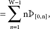
L1 = Length of queue when one server is working in the system 
L2 = Length of queue when two server is working in the system 
L3 = Length of queue when one server is working in the system 
23.4.3 Leisure Period and Working Period Length
The queue length of a busy one-time server one, busy two-time server, and busy three-time server are calculated. Since a working period is the addition of the leisure time, the busy time of 1 fixer, the busy time of 2 fixers, and the busy time of 3 fixers, EC = EB1 + EB2 + EB3 + EI
23.4.4 Cost of the System
Total expected cost during each unit of the M M 3 line system with a limited power L is measured. Here, {0, (q, r), W, S, T} are variable resolutions. In line with our goal of determining the maximum number of control variables, {(q, r), W, S, T} states (q⋆, r⋆, W⋆, S⋆, T⋆) to decrease the cost of the model.
The cost of the model is below.

Since the total amount of expected cost of work is unstructured, it is very tough to the correct values by analyzing reduction in the total cost of the expected cost over time for each unit. A specific search method can be used to find important results. In a search method, it is mandatory to have high limits for dynamic decisions and the search method can be discontinued after a complete global search in the internal area. The upper bound is L for the optimal values (q⋆, r⋆, W⋆, S⋆, T⋆).
Total cost function given in (23.31) is minimized by formulating the optimization problem

We use the advances optimization technique known as a Genetic Algorithm, which is a method based on genetic selection and genetic considerations. In a Genetic Algorithm, there are a bunch of all solutions to a problem. This solution then deals with regeneration and modification (as in original genes), produces new a child, and then repeats for different generations. Each person is alloted a qualifying value (based on the value of his or her goal) and the correct and suitable people are given a chance of getting married and giving more “worthy” people. This is in line with Darwin’s theory of “Survival of the Fittest”. In this way, we continue to “change” better people or solutions from generation to generation until we come to the point of deciding. The steps are as follows:
Getting started: enter value α, β, C, CV1, CV2, CV3, C01, C02, C03 C1, genes (Gq, Gr, GW, GM, GT), population size, probability and chance of conversion
Output: The standard solution is ![]()
Population: It is part of all possible (coded) solutions to a given problem. The first human population is a fixed G-length size with the genes Gq, Gr, GW, GM, and GT in the binary of 0 and 1 binary are generated randomly. The first human population that satisfies the inhibitory state (23.32) of each chromosome is produced randomly.
Calculation Qualification: The genetic value of each chromosome is calculated.
Choice: According to Darwin’s Theory “Survival of the Fittest”, the right amount was selected. Here, 3/4 of the population is selected for the next round according to their qualification value.
Crossover: During crossover, create new people by combining the characteristics of the people we have selected. If young people have a better fitness level, then the crossover operators will be killed. Here, we consider the 100% probability of a single point crossover method. Young people meet the conditions of the challenge.
Conversion: Conversion involves rearranging the list. Genetic modification is applied to each child after the crossover. The probability of conversion is 11% and we use the random value generated internally (0, 1). If the value is below the conversion rate, then it is slightly selected in the random area and its values are changed.
Stop: Step 4 to Step 7 is repeated until the stop conditions are met. Here, 50 repetitions are considered as stopping conditions. The above steps have been repeated 35 times.
MATLAB is used to configure programs. Assume the system volume is L = 20 and the cost of all lost customers is Cl = 50.
Sensitivity analysis is used for whole values based on changes in certain values.
The model has parameters α and β. The cost elements are as follows:
Case I: Ch = 100, C01 = 100, C02 = 200, C03 = 250, Cv = Cv1 + Cv2 + Cv3 = 300
Case II: Ch = 150, C01 = 100, C02 = 200, C03 = 300, Cv = Cv1 + Cv2 + Cv3 = 300
Case III: Ch = 100, C01 = 150, C02 = 250, C03 = 300, Cv = Cv1 + Cv2 + Cv3 = 500
Case IV: Ch = 100, C01 = 100, C02 = 200, C03 = 300, Cv = Cv1 + Cv2 + Cv3 = 400
Case V: Ch = 100, C01 = 100, C02 = 200, C03 = 300, Cv = Cv1 + Cv2 + Cv3 = 300
Case VI: Ch = 100, C01 = 100, C02 = 250, C03 = 300, Cv = Cv1 + Cv2 + Cv3 = 400
Case VII: Ch = 100, C01 = 100, C02 = 200, C03 = 400, Cv = Cv1 + Cv2 + Cv3 = 200
For all the costs listed above, optimal value and expected cost for different values of α are shown in Table 23.1. It is clearly seen that total cost increases as α increases. When all the servers are on vacation, Cv increases (See Case III & Case VII) as it includes the cost associated with Cl and holding cost of all failed machines in the system. Cost associated with higher threshold value is always increased.
Table 23.1 Expected cost E (q⋆, r⋆, W⋆, S⋆, T⋆) and optimal value (q⋆, r⋆, W⋆, S⋆, T⋆) (For α=4, 6, 7, 8, 9, 10).
| α | 4 | 6 | 7 | 8 | 9 | 10 | |
|---|---|---|---|---|---|---|---|
| I | q⋆, r⋆, W⋆, S⋆, T⋆ | 1,3,4,5,6 | 2,3,4,5,6 | 1,2,3,4,6 | 2,3,4,6,7 | 4,5,6,7,8 | 3,4,5,6,7 |
| E(q⋆, r⋆, W⋆, S⋆, T⋆) | 1099.89 | 1001.43 | 1003.90 | 1005.87 | 1006.34 | 1007.21 | |
| II | q⋆, r⋆, W⋆, S⋆, T⋆ | 2,3,4,5,6 | 1,2,3,4,6 | 3,4,5,6,7 | 2,3,4,5,8 | 3,4,5,6,8 | 4,5,6,7,8 |
| E(q⋆, r⋆, W⋆, S⋆, T⋆) | 1424.34 | 1461.45 | 1495.74 | 1501.21 | 1503.90 | 1505.43 | |
| III | q⋆, r⋆, W⋆, S⋆, T⋆ | 2,3,4,6,7 | 3,4,5,6,8 | 1,2,4,6,7 | 2,4,6,7,8 | 4,5,7,8,9 | 5,6,7,8,9 |
| E(q⋆, r⋆, W⋆, S⋆, T⋆) | 2007.39 | 2018.14 | 2100.56 | 3112.71 | 3413.20 | 3740.38 | |
| IV | q⋆, r⋆, W⋆, S⋆, T⋆ | 3,5,6,7,8 | 2,4,6,7,8 | 2,3,4,6,7 | 4,5,6,7,9 | 5,6,7,8,9 | 6,7,8,9,10 |
| E(q⋆, r⋆, W⋆, S⋆, T⋆) | 1004.13 | 1007.67 | 1011.31 | 1149.74 | 1179.89 | 1200.06 | |
| V | q⋆, r⋆, W⋆, S⋆, T⋆ | 3,4,7,8,9 | 4,5,6,7,9 | 2,5,7,8,9 | 6,7,8,9,10 | 4,6,8,9,10 | 5,7,8,9,10 |
| E(q⋆, r⋆, W⋆, S⋆, T⋆) | 1262.11 | 1342.03 | 1376.40 | 1428.29 | 1501.10 | 1503.29 | |
| VI | q⋆, r⋆, W⋆, S⋆, T⋆ | 4,5,6,7,8 | 3,4,5,7,9 | 4,5,7,8,10 | 5,6,7,9,10 | 6,7,8,9,10 | 5,7,8,9,10 |
| E(q⋆, r⋆, W⋆, S⋆, T⋆) | 1004.52 | 1007.21 | 1191.32 | 1134.69 | 1187.74 | 1200.54 | |
| VII | q⋆, r⋆, W⋆, S⋆, T⋆ | 5,7,8,9,10 | 6,7,8,9,10 | 4,6,8,910 | 5,7,8,9,10 | 4,5,8,9,10 | 5,6,7,8,10 |
| E(q⋆, r⋆, W⋆, S⋆, T⋆) | 1236.00 | 1332.39 | 1737.20 | 2429.31 | 2519.93 | 2739.71 |
23.5 Conclusions
The paper concluded the steady-state results for a multiserver queueing system with fixed capacity. A cost analysis is done to find the best level (q⋆, r⋆, W⋆, S⋆, T⋆) of breakdown machines in the system using a genetic algorithm. The flexibility of inclusion of servers increases the system efficiencies and avoids customer loss due to service delay. Cost analysis at different system parameters is useful for researchers and engineers.
References
- 1. Anupama and Solanki, A., “Performance Analysis And Optimization Of An M/M/3 Queuing System Under Tetrad Policy” International Journal of Advanced Technology in Engineering and Science (IJATES), ISSN: 2348 – 7550, ISSN (online): 2348 – 7550, Vol.02(11), pp 433-444, November 2014.
- 2. Bell CE (1971),” Characterization and computation of optimal policies for operating an M/G/1 queueing system with removable server”. Operations Research 19:2008–218.
- 3. Bell CE (1972).,” Optimal operation of an M/G/1 priority queue with removable server”. Operations Research 21:1281–1289.
- 4. Gnedenko et al. (1969),” Mathematical methods of Reliability Theory” Academic press, NewYork.
- 5. Hahn and Sivazlian (1990),” Distribution of the busy period in a controllable MM2 under the Triadic (0‚K‚N‚M) policy”, J. Appl. Prob., Vol. 27, pp.425-432.
- 6. K. H. Wang and B. D. Sivazlian (1989),” Reliability of a system with warm standbys and repairmen”. Microelectron. Reliab, 29, 849-860.
- 7. Kuo-Hsiung Wang and Ya-Ling Wang (2002),” Optimal control of an M/M/2 queueing system with finite capacity operating under the triadic (0‚Q‚N‚M) policy” Math Meth Oper Res 55:447–460.
- 8. M. N. Gopalan (1975),” Probablistic analysis of single server n-unit system with (n-1) warm standbys.” Oper Res. 23, 591-595.
- 9. M. Yadin and P. Naor (1963),” Queueing systems with a removable service station”. Opl Res. Q. 14, 393-4005.
- 10. M. J. Magazine (1971),” Optimal control of multi-channel service systems”. Naval Res. Logist. Q. 177-183.
- 11. M. J. Sobel (1969),” Optimal average-cost policy for a queue with start-up and shut-down costs”. Opns Res. 17, 145-162.
- 12. Rhee H-K, Sivazlian BD (1990),” Distribution of the busy period in a controllableM/M/2 queue operating under the triadic (0,K,N,M) policy”. Journal of Applied Probability 27:425–432.
- 13. R. Natarajan (1968),” A reliability problem with spares and multiple repair facilities”. Opns Res. 16, 1041-1057.
- 14. Subramanian et al. (1976),” Reliability of a repairable system with standbys failure.” Opns res. 24, 169-176.
- 15. Wang K-H, Huang H-M (1995),”Optimal control of a removable server in an M/Ek/1 queueing system with finite capacity”. Microelectronics and Reliability 35:1023–1030.
- 16. Wang K-H, Ke J-C (2000),” A recursive method to the optimal control of an M/G/1 queueing system with finite capacity and infinite capacity”. Applied Mathematical Modelling 24:899–914.
Note
- ⋆ Corresponding author: [email protected]