
2
Study of Lidar Signals of the Atmospheric Boundary Layer Using Statistical Technique
Kamana Mishra1⋆ and Bhavani Kumar Yellapragada2
1School of Mathematical and Statistical Sciences, Indian Institute of Technology Mandi, Himachal Pradesh, India
2Department of Space, National Atmospheric Research Laboratory Tirupati, India
Abstract
The rotational turbulence caused by mixing the layers of air, wind shear components, mountain waves, aerosol particles, and other pollutants affects the lowest and densest layer of the earth’s surface troposphere. Due to the turbulence, the height of the convective boundary layer (CBLH) changes over the day dramatically. We observe the variation in peak positions of lidar backscatter signals by performing a statistical technique for analyzing the behavior of the convective boundary layer (CBL). After that, to examine the behavior of the whole boundary layer, a distribution method and histogram plots will be used. We provide the statistical method for getting the best fit distribution to show how the result leads to the physical observation of data.
Keywords: Statistical technique, lidar data, distribution plots, convective boundary layer
2.1 Introduction
Surface forcing of the planetary boundary layer influences the closest and deepest part of the earth’s atmosphere, i.e., the troposphere. The turbulence in the troposphere causes the high variability of the temperature, moisture, wind shear, and pollutant particles. Due to surface friction, winds in ABL are weaker than above and tend to blow towards the area where pressure is low. It is noticeable over the Indian subcontinent that the height of the convective boundary layer (CBLH) is low during the winter and monsoon and high in the sunny days as the warmer lower-layer air mixes with the cool air and convection arises in the summertime only. This behavior indicates that solar heating affects the CBLH, and hence, CBL is also named the daytime planetary boundary layer. The convection occurs by mixing of airs forming bubbles of warmer air or eddies. The small eddies generated by the local wind shear cause turbulence in the surface layer and have a completely random behavior, however, the turbulence in the mixed layer is caused by large bubbles of warmer air, and hence, it is not completely random. Since the turbulent processes are found to be nondeterministic, it is beneficial to use a robust technique like statistical methods to find out the variability in the boundary layer and its key parameter as CBLH and has been studied by Pal, S., Behrendt, A., and Wulfmeyer V. in Elastic-backscatter-lidar-based characterization of the convective boundary layer and investigation of related statistics [3]. The signal which will be used in the study of CBLH is the total backscatter from the atmosphere that represents combined aerosol and molecular backscatter as mentioned earlier by Dang R, Yang Y, Hu X-M, Wang Z, and Zhang S [2]. For using the statistical method, we need the information in terms of data and we choose an instrument with high resolution power named Lidar (Light Detection and Ranging), which is a remote sensing method used in measuring the ranges to the earth and the concept of using Lidar to detect ABL height relies on the assumption that there is a strong gradient in the concentration of aerosols in the CBL versus the free atmosphere. The importance of defining a new technique is that this method works for single scan data and uses spatial average, however, the variance method needs multiple numbers of scans to identify the variance and use time average.
After finding the CBLH through statistical technique, we will try to examine the behavior of the whole boundary layer rather than just the CBL part. The histogram plots and distribution method can serve this purpose very well, meaning a list of best fit distribution along with each signal can be used to examine the behavior of the boundary layer, used before by the authors in ‘The Determination of Aerosol Distribution by a No-Blind-Zone Scanning Lidar” [6]. After getting the list of all possible distributions, it will be checked whether there is any range of the signals which follow a specified distribution or if the signals are following the distributions randomly. Now, to find the distribution of the backscatter signals manually for any structure of the boundary layer, a new technique needs to be introduced which holds in practical life. In this new technique, we will try to use the statistical approach. Lastly, we check the consistency for applying both the statistical techniques by using two different datasets and relate the mathematical result with the physical observations to examine the behavior of ABL.
2.2 Methodology
2.2.1 A Statistical Approach to Determine the CBLH
Due to the high-resolution power of Lidar, signals of Lidar can be used in finding the CBLH as Georgoulias, A.K., Papanastasiou, D.K., and Melas, D. et al. used in “Statistical analysis of boundary layer heights in a suburban environment” [4]. There are different types of Lidar techniques that serve a specific purpose, such as temperature profile using vibrational Raman (VR) and rotational Raman (RR). Backscattering Lidar and Elastic-backscatter Lidar (EBL) were used in ‘New Technique to Retrieve Tropospheric Temperature Using Vibrational and Rotational Raman Backscattering’ [5]. In our statistical technique, we do simple differentiation of the signal concerning the height, i.e., tracking the local maxima points, then we do some restrictions on the points of local maxima to indicate the real position of peaks of backscatter signal. The peak position changes with change in values of the restriction set. The peak position changes with change in values of the restriction set given below in Table 2.1.
Table 2.1 Restriction set used in algorithm for detecting peak position of lidar signals.
| Elements of set of restriction | Meaning | Default value |
|---|---|---|
| mph | Minimum peak height | None |
| mpd | Minimum distance between two peaks | 1 (positive integer) |
| threshold | Noise level | 0 |
| kpsh | Keep peaks with the same height even if they are closer than `mpd` | False |
| valley | Local minima | False |
2.2.2 A Statistical Approach to Determine the Best Fit Distribution to the Backscatter Signals of the Lidar Dataset
In this technique, we start with the histogram plots which help in deciding which type of distributions can take place and after that, a list of distributions will be prepared, which can be discrete or continuous. Now, to get the best fit distribution one needs to use tests under the null hypothesis to prove that this particular distribution holds well. There are many tests like the chi-square test for independence, ANOVA (analysis of variance), Homogeneity of Variance (HOV), Mood’s Median, Distance Covariance Test (d cov), Kolmogorov-Smirnov test (KS test), Welch’s T-test, Kruskal-Wallis H Test, etc. that are available to use but choosing a test is a crucial part of the procedure. So, after roughly looking at the histogram plots of the data and examining the previous research defined in “Analysis of ocean clutter for wide-band radar based on real data” [7], “A Speckle Filtering Method Based on Hypothesis Testing for Time-Series SAR Images” [8], “Structural Dynamics of Tropical Moist Forest Gaps” [9], and “Non-cooperative signal detection in alpha stable noise via Kolmogorov-Smirnov test” [10], it can be observed that the data follows continuous distribution and since the Kolmogorov-Smirnov test (KS test) can be applied only for the data which follows continuous distribution and has a limitation that the distribution must be fully specified, the k-s test is the best option according to our dataset. Now, after defining the list of possible distributions and choosing the test, the percentile bins will be defined so that we can make use of a particular range of the data rather than the exact dataset. An increment in the number of percentile bins results in a more accurate distribution type. That is why we check whether the result holds for a large number of bins or not. After that, observed frequency and expected frequency is calculated to formulate the chi-square statistics. The fitness of distributions will be sorted based on p-value, which is calculated from the hypothesis and the chi-square statistics. Since all the parameters are defined here, to use this test for a large number of columns a function can be created and by giving the number of columns, one can get the name of the best fit distribution. Now, we can plot the histogram with the best-fit distribution curve to check whether our formulation of function holds or not. One can also get distribution with its value of scale and shape parameters using the format function which will be helpful to make a graph of the distribution corresponding to its parametric values.
2.3 Mathematical Background of Method
This new technique of finding CBLH is defined on the behalf of mathematics and it will pave the way for using the statistical methods more often in the future for observing the behavior of atmospheric data. To use the statistical approach, a dataset of backscatter signals is required and Lidar helps us get this dataset. Detecting the peaks of the signals implies getting a set of those points from the Lidar dataset, at which there is a steep gradient and differentiation serves this purpose very well. Since the values of this dataset are completely random and defining a function is not possible at all, we find the points of local maxima through the graph. The slope is zero at the points where there is local maxima or minima. Let us define this collection of local maxima and local minima points by A and set of local maxima points by B. Now, let a ∈ A. If the slope is positive ∀ y ∈ (a-δ, a) and negative ∀ y ∈ (a, a+ δ), then a ∈ B and if the slope is negative ∀ y ∈ (a-δ, a) and positive ∀ y ∈ (a, a+ δ), then a ∈ AB. After getting elements of B, we will move to the next step which means checking whether the point of local maxima is peak or not because the first derivative has a downward zero-crossing at peak maximum. But, in real-life experiments there is some random noise that produces the false peak points and the result will be affected if we include these false positions of peaks also. To avoid this problem, one has to put some restrictions which are defined earlier in the methodology.
After that, a statistical technique will be used to find the distribution which fits best to the given data. The histogram is a helpful tool to figure out what kind of distribution data we have. Hence, by roughly analyzing the histogram plot, one can define a set of possible distributions (continuous or discrete) which can fit the data and choose the test accordingly. We will make use of the KS test here, which decides whether the sample comes from a population with specific distribution and is based on the empirical distribution function (ECDF). If N data points are given, then firstly order them from smallest to largest value, which can be denoted as X1, X2, …, XN. Then, ECDF can be defined as:
where n(i) is the number of points that are less than Xi.
K-S Test:
(Null hypothesis) H0: data follows given distribution
(Alternative hypothesis) H1: data does not follow the given distribution function
Test Statistic:
This test is defined as:
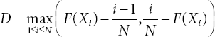
where F is the cumulative distribution function of the distribution that will be tested with the condition that it must be continuous distribution, as well as fully specified, which means parameters (such as local, shape, and scale) cannot be calculated from the dataset.
Significance level: α
Critical Value: We reject the null hypothesis if the value of D is greater than the critical value obtained from the table and this value can be written as a p-value.
So, a p-value based on the approximation of the distribution of the test statistics under the null hypothesis is calculated. Based on the p-values and chi-square statistics, we will sort the distribution starting from the best fit distribution. Since all the parameters have been termed, we can define a function using all these, send the value of the data column-wise, and then get the desired best fit distribution. One remark needs to be stated here: more than one distribution can be fit to the given pattern of data with a very small difference in their p-values. In that case, we can take the top three distributions and get a distribution that fits for some particular range of columns. This analysis emphasizes the databases with various forms of utterances in Tamil language for the applied classification technique and the obtained accuracy with the technique used to extract the feature. The number of samples which have been taken for this are tabulated in escalating order.
2.4 Example and Result
We will now consider an example of the Lidar dataset of backscatter signals of the boundary layer and scans are taken for every second for the time interval of ten minutes. In Figure 2.1, the temporal variation of Lidar signals shows the rise of boundary layer thermals. We have taken here the scans for a dataset in the interval 09:24-09:34. In ‘Analyzing the atmospheric boundary layer using high-order moments obtained from multiwavelength lidar data: impact of wavelength choice’ the authors have made the same figures for the larger time period from 13:00 to 19:00 UTC and from 17:00 to 21:00 UTC [1]. The reason for taking this time interval is that the turbulence in the CBL increases with the rise in sunrays, i.e., in the morning and due to the temperature variation boundary layer thermal increases. However, if we take the time-interval in the night, then turbulence ceases with the decrease in the amount of solar heating.

Figure 2.1 Temporal variation of lidar signal for dataset-1.
After using the statistical technique for all the backscatter signals, it is observed that after a certain height of signal, data behaves similarly for all the backscatter signals, which means the point at which there is a steep gradient approximately has the same location for each signal. This means that after a certain height of the layer, less presence of aerosols and other pollutant particle ceases the turbulence. Hence, a part of the backscatter signal in which the turbulence is very high is used rather than using the whole range. After getting the peak points for each scan, we make a graph of peak points along with scan number for a time-interval.
Now, if we compare these two figures, then it can be seen that the graph of peak points detected using the statistical technique matches the figure containing the rise of boundary layer thermals. When one observes graphs of the peak points for each signal in the included excel sheet, it can be easily seen that in starting there is a peak point near the first peak and after some signals, there is no point of the peak near the first peak point. Again, there is a peak point found near the first one which shows the dissimilarity in the location of peaks of the backscatter signals. From Figure 2.2, one can notice that peak points are randomly distributed over the interval. Also, the changes in peak height are not following any particular pattern. This result shows that the changes in the part of the surface layer of CBL do not follow any identified pattern and hence cannot be organized into any predefined structure.

Figure 2.2 Peak points with scan numbers for dataset-1.
However, after excluding a certain range, peak points attain the approximately same position, which physically shows that the turbulence above this shallow layer in the mixed layer is not completely random and can be organized into some predefined structure like plums and thermals. This method seems to be consistent and to confirm this we will take another dataset with the time interval 09:34-09:44, having the same interval length. The same process will be used here and after getting the peak points for each scan, we will make a graph of peak points for dataset-2 along with scan number. This method seems to be consistent and to confirm this we will take another dataset with the time interval 09:34-09:44, having the same interval length as shown in Figure 2.3. The same process will be used here and after getting the peak points for each scan, we will make a graph of peak points for dataset-2 along with the scan number as shown in Figure 2.4.
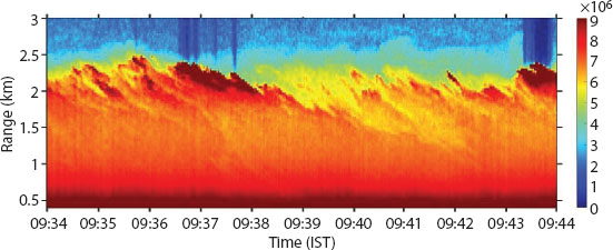
Figure 2.3 Temporal variation of lidar signal for dataset-2.

Figure 2.4 Peak points with scan numbers for dataset-2.
In this, if we compare both the figures then the peak points clearly show the temporal variation of Lidar signals. Hence, the result shows the consistency of the statistical method used here and this method can be utilized in detecting peak positions of backscatter signals.
After using the statistical technique (k-s test statistic), the distributions which fit the dataset of the backscatter signals have been found and a list of them along with the histogram plot, as well as the graph of best-fit distribution in an excel file are included in the link. Now, if we analyze the graphs up to the two-thirds part of the dataset, gamma or beta distribution fits in its maximum part, which has an almost same graph, and in the remaining one-third of the dataset, t-distribution fits perfectly. However, a few datasets perform the log norm, chi-square, inverse Gaussian, and Pearson 3 distributions. If we use the same technique for dataset-2 and analyze the graphs, the whole dataset follows t-distribution. This is probably happening because we have taken this dataset for the time-interval which is after the time for the first dataset.
2.5 Conclusion and Future Scope
The observations we have obtained using a statistical technique for the scans are the same as the temporal variation of Lidar signals. We have checked it using another dataset. Hence, the method gives a consistent result and can be utilized in detecting peak positions of backscatter signals. After that, we move to analyze the behavior of the whole boundary layer rather than only the CBL part using the distribution method for scans. Then, it is noticeable that the changes in the distribution with some particular ranges of signals are happening due to the physical process involved in that. Sometimes we get a broader spectrum and sometimes a narrower spectrum. The reason for this change is that the broader spectrum indicates turbulence process and wind variability, whereas the narrower spectrum indicates temperature inversion and is associated with stable layer phenomenon. The fitting of distribution is affected by thermal heating, water vapor condensation, and other physical processes involved during the day. So, we have examined the natural environment and now this study leads us to examine the changes in the manmade environment. The consistency of this method is paving the way to use it in different fields such as hydrodynamic modeling, storm surge modeling, etc.
Acknowledgement
I would like to express my gratitude to the team of Lidar project of NARL, Tirupati, India for providing the data for the research work.
References
- 1. de Arruda Moreira, G., da Silva Lopes, F. J., Guerrero-Rascado, J. L., da Silva, J. J., Arleques Gomes, A., Landulfo, E., and Alados-Arboledas, L., 07 Aug 2019. Analyzing the atmospheric boundary layer using high-order moments obtained from multi-wavelength lidar data: impact of wavelength choice, Atmos. Meas. Tech., 12, 4261– 4276, https://doi.org/10.5194/amt-12-4261-2019.
- 2. Dang R, Yang Y, Hu X-M, Wang Z, Zhang S, 2019. A Review of Techniques for Diagnosing the Atmospheric Boundary Layer Height (ABLH) Using Aerosol Lidar Data. Remote Sensing. 11(13):1590. https://doi.org/10.3390/rs11131590.
- 3. Pal, S., Behrendt, A., and Wulfmeyer, V., 2010. Elastic-backscatter-lidar-based characterization of the convective boundary layer and investigation of related statistics, Ann. Geophys., 28, 825–847, https://doi.org/10.5194/angeo-28-825-2010.
- 4. Georgoulias, A.K., Papanastasiou, D.K., Melas, D. et al., 2009. Statistical analysis of boundary layer heights in a suburban environment. Meteorol Atmos Phys 104, 103– 111. https://doi.org/10.1007/s00703-009-0021-z.
- 5. Su, J., McCormick, M. P., & Lei, L. (2020). New Technique to Retrieve Tropospheric Temperature Using Vibrational and Rotational Raman Backscattering. Earth and Space Science, 7. https://doi.org/10.1029/2019EA000817.
- 6. Wang, J.; Liu, W.; Liu, C.; Zhang, T.; Liu, J.; Chen, Z.; Xiang, Y.; Meng, X, 2020. The Determination of Aerosol Distribution by a No-Blind-Zone Scanning Lidar. Remote Sens. 12, 626. https://doi.org/10.3390/rs12040626.
- 7. QingWeiPing, 2011. Analysis of ocean clutter for wide-band radar based on real data https://doi.org/10.1145/2071639.2071669
- 8. Yuan, J.; Lv, X.; Li, R, 2018. A Speckle Filtering Method Based on Hypothesis Testing for Time-Series SAR Images. Remote Sensing, 10, 1383. https://doi.org/10.3390/rs10091383.
- 9. Hunter MO, Keller M, Morton D, Cook B, Lefsky M, Ducey M, et al. (2015) Structural Dynamics of Tropical Moist Forest Gaps. PLoS ONE 10(7): e0132144. https://doi.org/10.1371/journal.pone.0132144.
- 10. J. Luo, S. Wang, E. Zhang and J. Luo, 2015. “Non-cooperative signal detection in alpha stable noise via Kolmogorov-Smirnov test” 2015 8th International Congress on Image and Signal Processing (CISP), 2015, pp. 1464-1468, doi: 10.1109/CISP.2015.7408114.
Annexure
Flowchart and Algorithm for peak detection
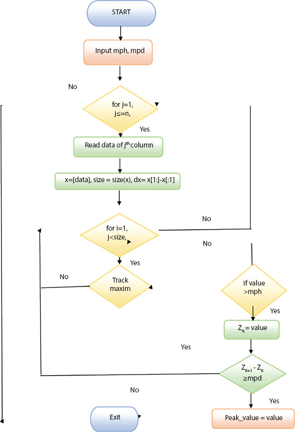
Flowchart:
Algorithm:
Step-1. Start Step-2. Input the minimum peak height (mph) and minimum distance between two peaks (mpd).
Step-3. Start a for loop to read columns of multidimensional data.
Step-4. Read the data of the column if ‘for’ loop is true else, go to step 11.
Step-5. Introduce a variable x to store the data in an array form. Then, use the size function to find the size of x and after that, use the differentiation function to differentiate the variable x.
Step-6. Again, start a ‘for’ loop for data stored in x.
Step-7. Track local maxima of data if for loop is true else, go to step 4 and restart the process for the next column.
Step-8. If it is a point of maxima then, check whether its value is greater than mph or not. If yes, go to step otherwise go to step 7.
Step-9. Introduce a new variable Zk and store the value in it.
Step-10. If difference between two local maxima i.e. Zk+1 - Zk is greater than mpd then, assign this value as peak value else go to step 7.
Step-11. Exit.
Algorithm for finding the distribution:
Step-1. Start.
Step-2. Make a function in which column number will be passed.
Step-3. Define a variable which takes the data of the column and size of the data.
Step-4. Input the list of possible distributions to find the best one among them.
Step-5. Input the number of percentile bins.
Step-6. Calculate the observed and expected frequency.
Step-7. Calculate the p-value by using the predefined Kolmogorov-Smirnov (KS) Test
Step-8. Calculate the value of chi-square statistics by using the formula as: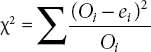 where Oi and are observed and expected frequencies respectively.
Step-9. Pass the number of columns in the function.
Step-10. Plot the histogram with the graph of best fit distribution for cross-checking the result.
Step-11. Stop.
Note
- ⋆ Corresponding author: [email protected]