Abstract

A production inventory model for a perishable good decaying at a constant rate has been devised in this research article. A ramp-type demand function has been considered, that is, the demand follows an accelerated growth initially for some time and finally becomes constant. The model allows shortage and is completely backlogged. The cost of holding the inventory is considered to vary linearly with time. Four cases have been developed depending on the position of time point at which the demand becomes constant in a trapezoidal-type demand. The production cycle restarts after a certain time. Optimal production stopping time and resuming time are calculated to optimize the expense of the production set-up per unit. The model is illustrated with a numerical.

Keywords: Trapezoidal demand, holding cost varying with time, completely backlogged short-ages, constant deterioration

17.1 Introduction

Demand is always fluctuating according to the requirements and preferences of customers and is quite unpredictable. In case of new launches of items like cosmetics, electronic gadgets with new technologies, trendy garments, etc. in the market, the items are in high demand initially. But, with the passage of time as more improvised items come into the market, the demand for the old ones become constant and stabilized. In order to deal with this kind of demand trend, trapezoidal demand has been dealt with in various studies since Ritchie (1980) [1]. Shaikh et al. (2020) [2] devised a stock optimization model for perishing goods with a preservation facility and a trapezoidal demand. Yang (2019) [3] developed an optimization model for a trapezoidal order trend having bi-level business credit type financing while placing orders. Chauhan et al. (2021) [4] developed an EOQ model for a trapezoidal type ordering system. During the stock out or shortage duration, backlogging is considered, also allowing certain discount strategies. Sana (2010) [5] considered deterioration and partial backlogging. Kawakatsu (2010) [6] devised an optimal refilling strategy for a retailer. A seasonal good with a trapezoidal order trend is considered with focus on Special Display Goods. Avinadav et al. (2013) [7] have developed a model where the demand varies with price of the item. Wang and Huang (2014) [8] devised a model for periodic items having price and trapezoidal-type order trends and deterioration. Ahmed et al. (2013) [9] proposed a fresh method for investigating the EOQ (Economic Order Quantity) assuming a trapezoidal demand, partial backlogging, and a general perish rate.

Perishing of items is an unavoidable phenomenon that should not be neglected while formulating an inventory system. But, it definitely depends on the kind of item taken into consideration. For example, for highly deteriorating items like fruits, vegetables, etc., deteriorating items should be taken as a variable function of time, quantity, etc. But, items such as metals (steel utensils, iron rods, etc.), medicines (expiry), etc. deteriorate extremely slow and hence the rate of deterioration might be considered constant. In this study, the items being studied are of the non-depreciating type like electronic goods, medicines, COVID protective gears, etc. In recent time, Halima et al. (2021) [10] devised an overtime production model for goods with a constant rate of perish and the demand depending on non-linear price and stock dependent order trend. Mandal and Pal (1998) [11] have developed inventory models for perishing goods that follows a trapezoidal demand.

Shortages of items are very common in the market system. When short-ages occur, it is completely a customer’s will whether to wait for the backorder or to go to some other seller for instant availability. Backlogging rate varies with the holdback time for the next refilling. Goyal (1988) [12] established a model for replenishment of trendy/fashionable inventories including shortages. Giri et al. (2000) [13] devised a model on lot sizing study for perishing goods with stockout situations and demand depending on time. Wang (2002) [14] devised a replenishment strategy for perishing items with inventory running with shortages and thus, partial backlogging. Ghosh and Chaudhuri (2005) [15] developed an economic order quantity model for a perishable good with trended demand and stockout situations in each cycle. Pentico and Drake (2011) [16] did a study on deterministic models for the economic order quantity models and economic production quantity models considering backordering. Sharma and Singh (2013) [17] devised a replica for perishable goods, accounting for consumption rate and backlogging. Roy Chowdhury et al. (2014) [18] designed an order-level inventory model for a decaying good having a quadratic type ordering pattern and backlogging during a stock out situation in every cycle. Tripathi (2015) [19] developed a model for perishing goods with an escalating order trend and stock out situation under inflationary spiral.

In the present work, a production-inventory model for a constantly perishable good with a trapezoidal-type order trend has been considered. The production starts at an initial time and is proportional to demand. The cost of holding inventory varies linearly with time. Shortage is allowed and is completely backlogged. Three cases have been dealt with depending on the position of the time at which the trapezoidal-type demand gains stability. We have illustrated the model numerically.

17.2 Assumptions and Notations

17.2.2 Notation

A: The unit ordering cost per cycle ($/unit)

P (t): Production rate varies directly with demand D(t), that is, P (t) = βD(t); this means that the higher the demand, the greater the production; this is required for ramp-type demand as initially demand is more, hence production should also be more to satisfy the customer demand, but the demand stabilizes after sometime and the production has to be reduced accordingly in order to avoid wastage of items and loss

ν: The parameter of the trapezoidal demand function (time point) where demand becomes constant

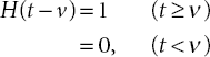
D(t): In case of certain items like COVID gear, with the outbreak of COVID-19 in India in the year 2020, the demand of masks and PPEs saw an increasing demand in the beginning but after some time the demand became stabilized. This kind of demand is a ramp type demand which can be mathematically expressed as: Demand at the time t ≥ 0

(17.1)

where H(t − ν) is a Heviside function defined as

(17.2)

C_O: Overall ordering expense

C_H: Overall holding expense

C_P: Overall production expense

C_D: Overall deterioration expense

C_S: Overall shortage expense

c_h: Time dependent Holding Cost (h+st) in the time interval [0, t₂]

c_p: Unit production expenses per item per unit time ($/unit/unittime)

c_d: Expenses of deterioration per item per unit time ($/unit)

c_s: Shortage expenses per unit per unit time

θ: Constant deterioration rate of the item, where 0 < θ ≪ 1

T: Total time period of the inventory cycle

ATC: Optimum aggregate total expense per unit time of the production-inventory system calculated using the optimized values of manufacturing end time, the instant when the stock exhausts, and the production resuming time

t_a: Time instant when the production ceases

t_b: Time instant when the inventory level gets exhausted in an unproductive state

t_c: Time at which the production starts again

17.3 Formulation and Solution

The present article develops a production inventory system for a perishable item decaying at a constant rate. The cycle begins with no items in the inventory, that is, the stock level is zero. The production P initiates at time t = 0 and pauses at time t = t_a. Demand is ramp-type and starts along with production. Within the time interval, 0 ≤ t ≤ t_a, the inventory builds up at a rate governed by the rate of production, the rate at which the orders are placed, and constant deterioration θ. The deterioration is acting on the accumulating inventory. In the interval t_a ≤ t ≤ t_b, the demand and the constant deterioration cause the inventory to deplete down to zero level at t = t_b. After this point, the shortage is allowed and is completely backlogged. As a result, the demand accumulates until t = t_c. Here, the production restarts to satisfy the backlogged demand as well as meet the current demand. t_a, t_b, and t_c are the decision variables. The cycle recurs after period T.

Depending on the position of the time point µ on the time horizon (0 < t < T ), we consider the following three cases:

1. 0 < ν < t_a < t_b < t_c < T
2. 0 < t_a < ν < t_b < t_c < T
3. 0 < t_a < t_b < ν < t_c < T

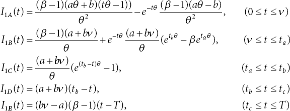
17.3.1 Case 1 i) 0 < ν < t₁ < t₂ < t₃ < T

The formulation of the production model is as follows:

(17.3)

with boundary conditions I_1A(0) = 0, I_1A(ν) = I_1B(ν), I_1B(t_a) = I_1C(t_a), I_1C(t_b) = 0, I_1D(t_b) = 0, and I_1E(T ) = 0.

The above differential equations have been solved to get the following expressions:

(17.4)

The total expenditure of the production inventory system comprises of:

1. Ordering Cost (C_O) = A.
2. Holding Cost
   (17.5)
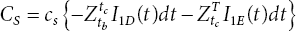
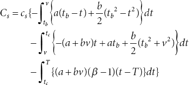
3. Shortage Cost
   (17.6)
4. Production Cost
   (17.7)
5. Deterioration Cost = (Production - Demand) in the time period (0, t_b)
   (17.8)

17.3.2 Case 2 ii) 0 < t_a < ν < t_b < t_c < T

The formulation of the inventory model is as follows:

(17.9)

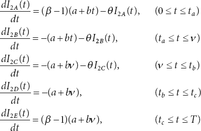
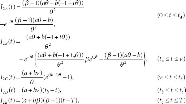
with boundary conditions being I_2A(0) = 0, I_2A(t_a) = I_2B(t_a), I_2B(ν) = I_2C(ν), I_2C(t_b) = 0, I_2D(t_b) = 0, I_2E(T ) = 0,

The above differential equations have been solved to get the following expressions:

(17.10)

1. Ordering Cost (C_O) = A.
2. Holding Cost
   (17.11)
3. Shortage Cost
   (17.12)
4. Production Cost
   (17.13)
5. Deterioration Cost = (Production - Demand) in the time period (0, t_b)
   (17.14)

17.3.3 Case 3 iii) 0 < t_a < t_b < ν < t_c < T

The formulation of the above production inventory model is as follows:

(17.15)

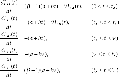
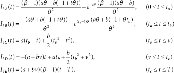
Boundary conditions: I_3A(0) = 0, I_3A(t_a) = I_3B(t_a), I_3B(t_b) = 0, I_3C(t_b) = 0, I_3C(ν) = I_3D(ν), I_3E(T) = 0,

The above differential equations have been solved to get the following expressions:

(17.16)

1. Ordering Cost (C_O) = A.
2. Holding Cost
   (17.17)
3. Shortage Cost
   (17.18)
4. Production Cost
   (17.19)
5. Deterioration Cost = (Production - Demand) in the time period (0, t_b)
   (17.20)

The average total system expenditure for the above three instances is given by:

The total system cost TC depends on three variables t_a, t_b, and t_c. We need to find the optimized values of t_a, t_b, and t_c that is, t^m, t^m, and t^m respectively, that minimize the average total system cost.

t^m, t^m, and t^m are the solution of respectively,

which are the necessary conditions for the optima. The sufficient conditions that minimize the average total cost are the Hessian Matrix H > 0 at t^m, t^m, t^m, where

(17.21)

17.4 Numerical Example

Example 1: Case 1 (0 < µ < t_a < t_b < t_c < T)

We now illustrate the above developed production inventory model with a numerical example. Random data taken are as follows: A = 100, Cd = 10, a = 70, b = 20, β = 0.001, θ = 0.001, Cs = 15, T = 8, ν = 5.6, Cp = 10, e = 2.718, h = 5, s = 0.05 (with appropriate units).

We use MATHEMATICA 7.0 to calculate the optimized values . The optimized values of t_a, t_b, t_c are units and the optimized average expense is ATC = 15, 613 units.

Example 2: Case 2 (0 < t_a < µ < t_b < t_c < T)

We now illustrate the above developed production inventory model with a numerical example. Random data taken are as follows: A = 100, Cd = 10, a = 70, b = 20, β = 0.001, θ = 0.001, Cs = 15, T = 8, ν = 5.7, Cp = 10, e = 2.718, h = 4, s = 0.04 (with appropriate units).

We use MATHEMATICA 11.3 to calculate the optimized values . The optimal values of t_a, t_b, t_c are units and the optimized average expense is ATC = 16, 041 units.

Example 3: Case 3 (0 < t_a < t_b < µ < t_c < T)

We now illustrate the above developed production inventory model with a numerical example. Random data taken are as follows: A = 100, Cd = 10, a = 80, b = 10, β = 0.001, θ = 0.001, Cs = 20, Ch = 4, T = 8, ν = 7.42, Cp = 10, e = 2.718, h = 5, s = 0.04 (with appropriate units).

We use MATHEMATICA 11.3 to calculate the optimized values . The optimal values of units and the optimized average expense is ATC = 1, 47, 896 units.

17.5 Discussion

Case 1: (0 < µ < t_a < t_b < t_c < T)

Here, ν < t_a and this implies that the demand curve becomes constant before the production stops (t_a = 7.2). Hence, the manufactured items will take some time to sell and the inventory level will fall to zero after some delay. This aspect is clear from the optimum values received in Example 1.

Case 2: (0 < t_a < µ < t_b < t_c < T)

Here, t_a < ν < t_b and this implies that the demand curve becomes constant after the production stops (t_a = 5.618). After the stabilization of demand, the level of the inventory reduces at a very slow rate. Hence, the level reduces to zero after a long duration at t_b = 8.05. This is clear from the optimum values of t_b, t_c received in Example 2.

Case 3: (0 < t_a < t_b < µ < t_c < T)

Here, t_b < ν and this implies that the demand curve is stabilized after the inventory level dips below the zero mark and the shortage begins. Because the inventory is running in shortage, therefore the optimal time to start the production is almost immediately. This aspect is clear from the optimum values in Example 3.

17.6 Inference

This study deals with a production-reserve (stock) model with a trapezoidal-type demand for an item that perishes constantly and inventory that is stored at a flexible cost. Shortages have been considered. The items considered are the ones like COVID gear (masks, PPE kits, etc.). Three cases have been discussed related to the demand change time and the inventory levels and production start and stop times. The decision variables are the production halt/break off time (t_a), the time at which the stock gets exhausted (t_b), and production restart time (t_c). In the future, this study can be taken further by considering a flexible deterioration rate.

References

1. 1. E. Ritchie Practical inventory replenishment policies for a linear trend in demand followed by a period of steady demand J. Oper. Res. Soc., 31 (7) (1980), pp. 605-613.
2. 2. An inventory model for deteriorating items with preservation facility of ramp type demand and trade credit Ali Akbar Shaikh, Gobinda Chandra Panda, Md. Al-Amin Khan, Abu Hashan Md. Mashud, Amiya Biswas https://doi.org/10.1504/IJMOR.2020.110895 International Journal of Mathematics in Operational Research Volume 17, Issue 4, 2020.
3. 3. Open Journal of Business and Management, Vol.7 No.2, April 2019 An Inventory Model for Ramp-Type Demand with Two-Level Trade Credit Financing Linked to Order Quantity Hui-Ling Yang DOI: 10.4236/ ojbm.2019.72029
4. 4. Chauhan et al. [2021] An order quantity scheme for ramp type demand and back-logging during stock out with discount strategy, Anand Chauhan, Shilpy Tayal, https://doi.org/10.1504/IJSOI.2021.114113 International Journal of Services Operations and Informatics Volume 11, Issue 1
5. 5. Sana, S., (2010), ‘Optimal selling price and lotsize with time varying deterioration and partial backlogging’, Appl. Math. Comput., Vol. 217, pp. 185-194.
6. 6. H. Kawakatsu, Optimal retailers replenishment policy for seasonal products with ramp-type demand rate, IAENG Int. J. Appl. Math. 40 (4) (2010) 17.
7. 7. Avinadav, T., Herbon, A., Spiegel, U. 2013. Optimal inventory policy for a perishable item with demand function sensitive to price and time. Int. J. Production Economics 144, 497506.
8. 8. Pricing for seasonal deteriorating products with price-and ramp-type time-dependent demand C Wang, R Huang - Computers & Industrial Engineering, 2014 - Elsevier
9. 9. M.A. Ahmed, T.A. Al-Khamis, L. Benkherouf Inventory models with ramp type demand rate, partial backlogging and general deterioration rate Appl. Math. Comput., 219 (2013), pp. 4288-4307.
10. 10. Alexandria Engineering Journal Volume 60, Issue 3, June 2021, Pages 2779-2786 An over-time production inventory model for deteriorating items with nonlinear price and stock dependent demand Mohammad Abdul Halima A.Paul MonaMahmoud B.Alshahranic Atheelah Y.M.Alazzawi Gamal M.Ismaile
11. 11. Mandal, B., Pal, A.K., 1998. Order level inventory system with ramp type demand rate for deteriorating items. Journal of Interdisciplinary Mathematics 1 (1), 4966.
12. 12. Goyal, S.K., (1988), ‘A heuristic for replenishment of trended inventories considering shortages’, Journal of the Operational Research, Vol.39, pp.885-887.
13. 13. Giri, B.C., Chakraborty, T., Chaudhuri, K.S., (2000), ‘A note on a lot sizing heuristic for deteriorating items with time-varying demands and shortages’, Computers and Operations Research, Vol.27, pp.495-505.
14. 14. Wang, S.P., (2002), ‘An inventory replenishment policy for deteriorating items with shortages and partial backlogging’, Computers & Operations Research, Vol.29(14), pp.2043-2051.
15. 15. Ghosh, S.K., Chaudhuri, K.S., (2005), ‘An EOQ model for a deteriorating item with trended demand and variable backlogging with shortages in all cycles’, Int. J. Adv. Model. Optim. (Buchar. Rom.), Vol.7(1), pp.57-68.
16. 16. Pentico, D.W., Drake, M.J., (2011), ‘A survey of deterministic models for the EOQ and EPQ with partial backordering’, European Journal of Operations Research, Vol. 214(2), pp. 179-198.
17. 17. Sharma, S., Singh, S.R., (2013), ‘An inventory model for decaying items, considering multi variate consumption rate with partial backlogging’, Indian Journal of Science and Technology, Vol. 6(7), pp.4870-4880.
18. 18. Roy Chowdhury, R., Ghosh, S.K., Chaudhuri, K. S., (2014), ‘An Order-Level Inventory Model for a Deteriorating Item with Time-Quadratic Demand and Time-Dependent Partial Back-logging with Shortages in All Cycles’, American Journal of Mathematical and Management Sciences, vol.33(2), pp.75-97.
19. 19. Tripathi, R.P., (2015), ‘Economic order quantity for deteriorating item with nondecreasing demand and shortages under inflation and time discounting’, International Journal of Engineering, Vol.28(9), pp.1295-1302.