Abstract

This paper aims to address the problem with viscolelastic p-Laplacian type equations with logarithmic nonlinearity,

in which p ≥ 2, under a convenient hypotheses on g (t). Under suitable conditions, we discuss global existence and blow up the results.

Keywords: Existence, blow up, viscoelastic equation, p–Laplacian type equation, logarithmic nonlinearity

21.1 Introduction

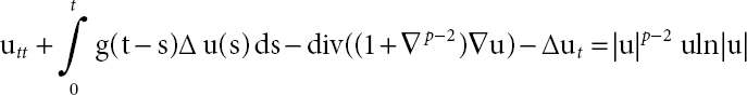
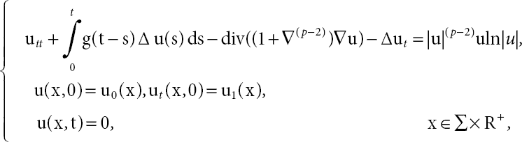
Let Ω be a bounded domain in Rⁿ (for n ≥ 1) with smooth boundary Σ = ∂Ω. We deal with the following problem in the initial boundary problem for (x, t) ∈ Ω × R⁺:

The memory kernel g(t) is a real function which has typical properties. In (21.1), if we take ln |u| = 1 and replace the second order as the fourth order, we have

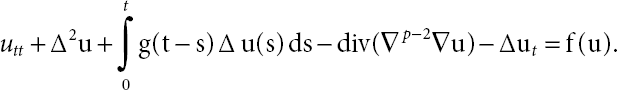
Equation (21.2) was named as a fourth order weak viscoelastic plate equation with a lower order perturbation of p-Laplacian type and it can be taken as a general form of the one-dimensional nonlinear equation of elastoplastic microstructure flows. This type of equation was first considered by Andrade et al. [3]. They deal with interplay of the p-Laplacian operator with viscoelastic terms. The authors obtained existence and decay results of solutions with g^t(t) ≤ cg (t). Later results about qualitative theory results of solutions to (21.2) type equations were obtained by different authors (see [4, 13, 14, 18, 19, 26]).

The logarithmic wave equations which were introduced by Bialynicki-Birula and Mycielski in [5] are related with many areas of physics. Logarithmic source term occurs naturally in inflation cosmology and quantum mechanics, supersymmetric field theories, and nuclear physics [7, 17]. Later, by the motivation of these works, analysis of logarithmic source terms attracted many authors (see [8−10, 16, 23, 25, 32, 35]). There is some work about mathematical behavior in viscoelasticity with logarithmic source terms. The references were given in our work for interested readers (see [2, 6, 11, 12, 20, 31]).

The model (21.1) for g = 0 and without ∆u was studied, but there is not a substantial number of work related with p-Laplacian hyperbolic type equations. For contact problems on p-Laplacian type equations with logarithmic source terms see ([15, 24, 30, 33, 34]).

The goal of our work is to prove the global existence of a weak solution to the problem (21.1). Blow up results were established for suitable conditions at E (0) < d. As far as know, there is no work which is related on p-Laplacian hyperbolic type equations with viscoelastic terms and logarithmic source terms.

The structure of the work is as follows: to understand the expression in the work more easily, firstly we give some definitions, notations, energy functions, and some lemmas which will be used in our proof in Section 21.1. In part 2 and part 3, global existence results and blow up results were stated for the solution of problem (21.1), respectively.

21.2 Preliminaries

In this part, we consider the notation and some well-known lemmas. We define the inner product as

in Standard Lebesque Space L² (Ω) and we denote:

in . The norm in L² (Ω) and L^p (Ω) will be defined by ǁ.ǁ and ǁ.ǁ p. And C will be various positive constants.

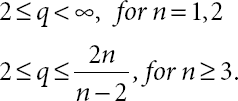
Lemma 21.1. [1, 22] Let q be a positive number, which implies that

So, for we have

(21.3)

where C_q is a positive constant.

Now, we will consider some assumptions based on the kernel function g(t):

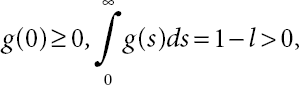
(A1) In accordance with g: [0, ∞) → R⁺ (g(t) is a nonnegative function), we suppose that the function g ∈ C¹ [0, ∞) and

(21.4)

(A2) Let ϑ be a positive number which satisfies for t ≥ 0

(21.5)

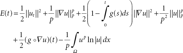
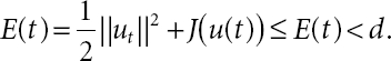
E(t) will be denoted total energy functional for the model investigated in (21.1). It follows that

(21.6)

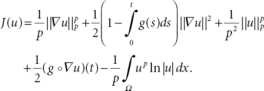
We introduce the J(u) as a potential energy functional so that

(21.7)

We obtain for

(21.8)

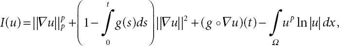
where

(21.9)

Then, it is clearly concluded that for

(21.10)

(21.11)

According to potential well theory, the set stability for the problem (21.1) was considered as:

(21.12)

So, we denote outer space of the potential well by

(21.13)

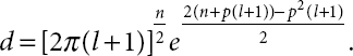
The potential well depth can be considered as:

(21.14)

Similar to the result in [29], one has:

Where according to the potential functional, well-known Nehari Manifold N is given by:

Now, we state some definitions and lemmas. Lemma 21.5 and Lemma 21.6 are related with potential well theory results.

Lemma 21.2. [21]. Suppose that u is a function which satisfies and a is defined as positive number. Then,

Definition 21.3. Let T > 0 and u be defined as the solution of problem (21.1). If u holds

and

for each test functions then u will be taken as a weak solution for the (21.1).

Lemma 21.4. Assume that (A1) and (A2) conditions, which are related with g(t) functional, hold. Then, the total energy of problem (21.1) decreases over respect to t because

(21.15)

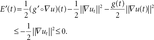
where

(21.16)

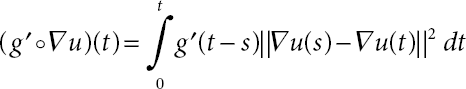
Proof. First, we multiply both sides of the equation by u_t in the (21.1) equation. Later, by integrating over t it yields that

(21.17)

Here, by direct calculations we obtained (21.16).

Lemma 21.5. For any and it gives

1. 
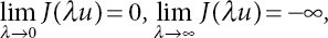
2. For 0 < λ < ∞ we find a unique λ^⋆ such that
3. For 0 < γ ∞ we find a unique γ^⋆ such that
   
4. J (λu) functional is strictly decreases on λ^⋆ < λ < ∞, increases on 0 < λ < λ^⋆ and attains the maximum at λ = λ^⋆ and I (λu) > 0 for 0 < λ < λ^⋆, I (λu) < 0 for λ^⋆ < λ < ∞ and the Nehari functional I(λ^⋆u) = 0, where

Proof.

1. Thanks to the definition of J(u), we conclude that
   (21.18)

   It is easy to get from that is

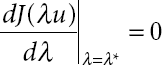
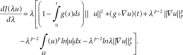
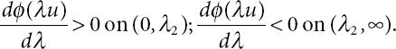
2. Now, differentiating J (λu) with respect to λ, it yields that
   (21.19)

   Let 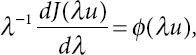so we obtain

   

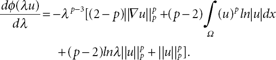
   Let 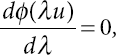0 which implies

   

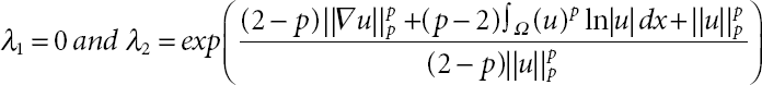
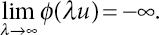
   An elementary calculation shows that

   

   We observe from 2 ≤ p that so that there is exactly ϕ(λ^⋆u) = 0, which means

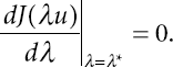
3. A simple corollary of the (ii) directly follows from
   (21.20)

Lemma 21.6. Assume that and Then, we obtain where

Proof. If I(λ^⋆u) = 0 and from Lemma 21.4 and Equation (21.10), we obtain

(21.21)

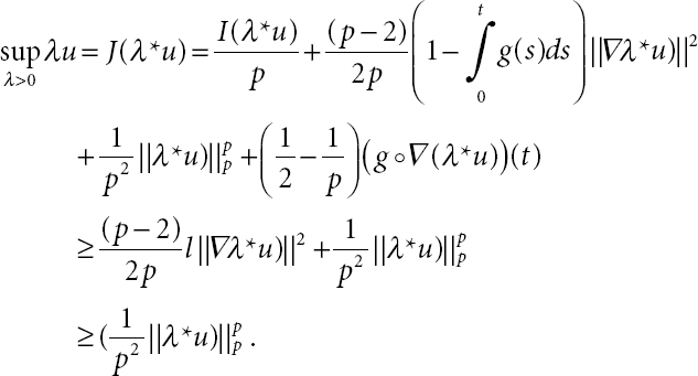
Since now by using the following inequality

we have

(21.22)

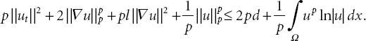
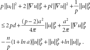
By using L^p Logarithmic Sobolev inequality and definition of I(u) and (21.22), we get

(21.23)

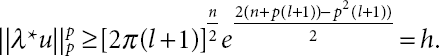
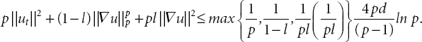
Taking we find

(21.24)

From I(λ^⋆u) = 0 and (21.24), we conclude that

which satisfies that

(21.25)

Thus, by combining (21.21) and (21.25), we obtain

21.3 Global Existence Result

This part is related to global existence results. We established that the solutions will exist globally for problem (21.1) for the case 0 < E(0) < d by considering the following lemma to state proof of Theorem 21.8.

Lemma 21.7. Assume that Let initial energy holds 0 < E(0) < d. Moreover, u ∈ U where u is taken as a weak solution of Equation (21.1).

Proof. For 0 < E(0) < d, we claim that u was taken as a weak solution for Equation (21.1). Now, we will use the contradiction method. We suppose that u ∉ U and t^⋆ are the smallest time of u (t^⋆) ∉ U. By continuity of u(t), we know clearly that u(t^⋆) ∈ ∂U and u ∈ U for t ∈ [0, t^⋆). By virtue of the definition of U and the continuity of I(u) and J(u) about time, we have either J(u(t^⋆)) = d or I(u(t^⋆)) = 0. Thanks to Lemma 21.3, it follows that

(20.4)

Therefore, it is clear that the former case is not possible. Suppose that I(u(t^⋆)) = 0, then u (t^⋆) ∈ N. By the definition of d, J(u (t^⋆)) ≥ d was obtained, which is in contradiction with J(u (t^⋆)) < E(0) < d. So, we showed that the other case is not possible as well.

Theorem 21.8. Let Then, Equation (21.1) with initial boundary conditions has a global weak solution with u_tt under the condition 0 < E (0) < d.

Proof. Our purpose is to prove that is bounded for not depending on t. By using Lemma 21.4, (21.11), definition of E(t), and the condition 0 < E(0) < d, we obtain

(21.27)

According to conditions in Theorem 21.8, by using Lemma 21.7, for t ≥ 0 we obtain

(21.28)

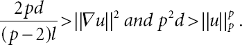
We conclude from (21.10) and (21.28) that

(21.29)

which implies that

(21.30)

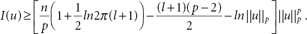
It follows from (A1), the definition of J(u), (21.11), and (21.27) that

(21.31)

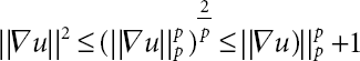
By using Lemma 21.1, (21.31) shows that

(21.32)

Let , then by using Lemma 21.6 and (21.30), (21.32) becomes

(21.33)

which satisfies that

(21.34)

Therefore, we have solutions (u) for the Equation (21.1) that exist globally, by using (21.34) and by the same argument, the continuation theorem [27, 28].

21.4 Blow Up Results of the Solution for Equation (21.1)

This section is related to blow up results for Equation (21.1) at infinity. We state some lemma which will be useful for our proof. Proof Lemma 21.9 can be obtained by same argument as Lemma 21.7.

Lemma 21.9. Let u be taken as a weak solution of Equation (21.1). Suppose that and 0 < E(0) < d. Therefore, we have u ∈ V and E(t) < d.

Theorem 21.10. Let and and . u₀ ∈ V and E (0) < d, then the solution u of Equation (21.1) goes to the infinity when t → ∞, i.e.,

Proof. Under the conditions of Theorem 21.10, we conclude that I(u) is decreasing with respect to t, thank to results of the Lemma 21.9. Thus, we can find for all t > 0

(21.35)

By using the Logarithmic Sobolev inequality, (21.35) can be written as

(21.36)

Since by using (21.22), we have

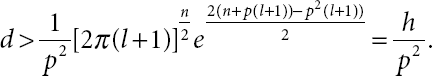
By taking into (21.36) and using definition of d, we introduce that

(21.37)

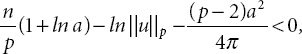
which satisfies that

(21.38)

Now, we set the functional G(t): [0, ∞) → R⁺ which was defined by

(21.39)

Direct computation on (21.39) leads to

(21.40)

By using Equation (21.1), we have second-order differentials of G(t) as follows:

(21.41)

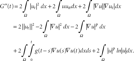
Since

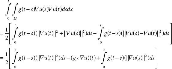
(21.41) leads to

(21.42)

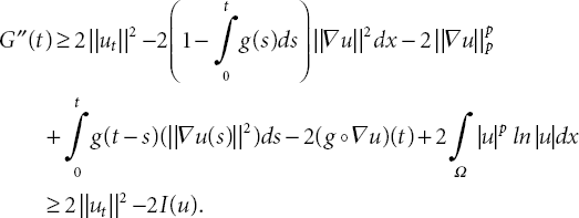
By combination of (21.39), (21.40), and (21.42) we obtain that

(21.43)

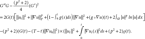
where

(21.44)

Thanks to the Cauchy-Schwarz inequality and Young inequality, the last term of ϱ(t) can be rewritten as

(21.45)

(21.46)

and

(21.47)

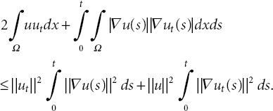
Moreover, by inserting (21.45)-(21.47) into (21.44), it is clearly seen that ϱ(t) ≥ 0. Depending on this interest, we replace (21.43) as

(21.48)

where Λ = Λ(t) is defined such that

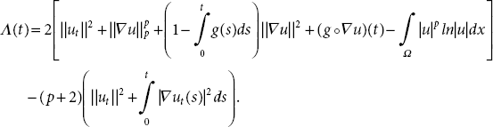
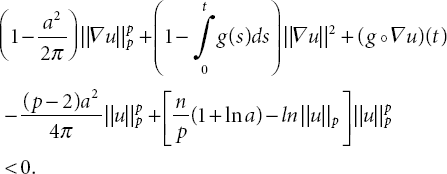
By using definition of total energy E(t), (A1), (A2), (21.22) and the Logarithmic Sobolev inequality, it follows that

(21.49)

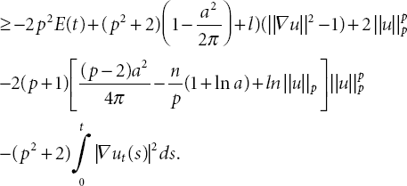
By , (21.37), (21.38), and (21.15), (21.49) can be found as

(21.50)

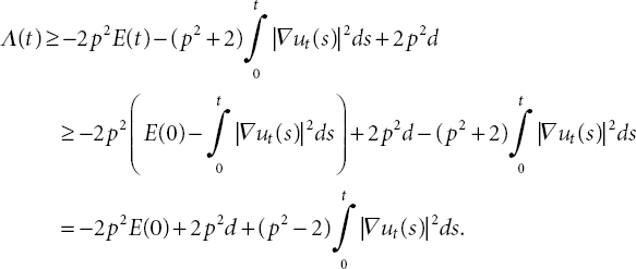
Therefore, we obtain from the condition of Theorem 21.10 (E (0) < d)

(21.51)

Therefore, by Inequality (21.51) and condition of the functional G(t), (21.48) yields that

(21.52)

By directly calculation of (21.52), it follows that

(21.53)

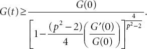
By integrating both sides of Inequality (21.53) over [0, t] for p > 2, it yields that

(21.54)

From definition of G(t), it is clear to conclude that 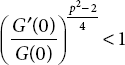where Consequently, we can rewrite (21.54) so that

Therefore, for some T^⋆ satisfies

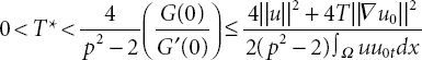
which means that

so that our solution blows up at T^⋆. This finishes the proof.

References

1. 1. Adams, R. A., Fournier, J. J. Sobolev spaces. Pure and applied mathematics (Amsterdam), (2003).
2. 2. Al-Gharabli, M. M., Al-Mahdi, A. M., Messaoudi, S. A. Decay Results for a Viscoelastic Problem with Nonlinear Boundary Feedback and Logarithmic Source Term. Journal of Dynamical and Control Systems, 1-19, (2020).
3. 3. Andrade, D., Silva, M. J., Ma, T. F. Exponential stability for a plate equation with p-Laplacian and memory terms. Mathematical Methods in the Applied Sciences, 4(35), 417-426, (2012).
4. 4. Araújo, G. M., Araújo, M. A. F., Pereira, D. C.On a variational inequality for a plate equation with p-Laplacian end memory terms. Applicable Analysis, 1-14, (2020).
5. 5. Bialynicki-Birula, I., Mycielski, J. Wave equations with logarithmic nonlinearities. Bull. Acad. Pol. Sci. Cl, 3(23), 461-466, (1975).
6. 6. Bouhali, K., Ellaggoune, F. Viscoelastic wave equation with logarithmic nonlinearities in Rn. J Partial Differ Equ, 30(1), 47-63, (2017).
7. 7. Buljan, H., Šiber, A., Soljačíc, M., Schwartz, T., Segev, M., Christodoulides, D. N. Incoherent white light solitons in logarithmically saturable noninstantaneous nonlinear media. Physical Review E, 68(3), 036607, (2003).
8. 8. Cazenave, T., Haraux, A. Équations d’évolution avec non linéarité logarithmique. In Annales de la Faculté des sciences de Toulouse: Mathématiques, 2(1), 21-51, (1980).
9. 9. Di, H., Shang, Y., Song, Z. Initial boundary value problem for a class of strongly damped semilinear wave equations with logarithmic nonlinearity. Nonlinear Analysis: Real World Applications, 51, 102968, (2020).
10. 10. Ding, H., Wang, R., Zhou, J. Infinite time blow-up of solutions to a class of wave equations with weak and strong damping terms and logarithmic nonlinearity. Studies in Applied Mathematics, 147(3), 914-934, (2021).
11. 11. Ferreira, J., Irkıl, N., Raposo, C. A. Blow up results for a viscoelastic Kirchhoff-type equation with logarithmic nonlinearity and strong damping. Mathematica Moravica, 25(2), 125-141, (2021).
12. 12. Ha, T. G., Park, S. H. Blow-up phenomena for a viscoelastic wave equation with strong damping and logarithmic nonlinearity. Advances in Difference Equations, 2020 (1), 1-17, (2020).
13. 13. Liu, W., Yu, J. On decay and blow-up of the solution for a viscoelastic wave equation with boundary damping and source terms. Nonlinear Analysis: Theory, Methods Applications, 74(6), 2175-2190, (2011).
14. 14. Liu, W., Li, G., Hong, L. Decay of solutions for a plate equation with p-Laplacian and memory term. Electronic Journal of Differential Equations, 2012(129), 1-5, (2012).
15. 15. Liu, C., Ma, Y. Blow up for a fourth order hyperbolic equation with the logarithmic nonlinearity. Applied Mathematics Letters, 98, 1-6, (2019).
16. 16. Ma, L., Fang, Z. B. Energy decay estimates and infinite blow-up phenomena for a strongly damped semilinear wave equation with logarithmic nonlinear source. Mathematical Methods in the Applied Sciences, 41(7), 2639-2653, (2018).
17. 17. De Martino, S., Falanga, M., Godano, C., Lauro, G. Logarithmic Schrödingerlike equation as a model for magma transport. EPL (Europhysics Letters), 63(3), 472, (2003).
18. 18. Park, S. H. Stability for a viscoelastic plate equation with p-Laplacian. Bulletin of the Korean Mathematical Society, 52 (3), 907-914, (2015).
19. 19. Pereira, D. C., de Araújo, G. M., Raposo, C. A.. Unilateral Problem for a Viscoelastic Beam Equation Type p-Laplacian with Strong Damping and Logarithmic Source. European Journal of Mathematical Analysis, 2 (5), 1-20, (2022).
20. 20. Peyravi, A. General stability and exponential growth for a class of semi-linear wave equations with logarithmic source and memory terms. Applied Mathematics and Optimization, 81(2), 545-561, (2020).
21. 21. Del Pino, M., Dolbeault, J., Gentil, I. Nonlinear diffusions, hypercontractivity and the optimal Lp-Euclidean logarithmic Sobolev inequality. Journal of Mathematical Analysis and Applications, 293(2), 375-388, (2004).
22. 22. Pişkin, E., Okutmuştur, B. An Introduction to Sobolev Spaces, Bentham Science, (2021).
23. 23. Pişkin, E., Irkıl, N. Well-posedness results for a sixth-order logarithmic Boussinesq equation. Filomat, 33(13), 3985-4000, (2019).
24. 24. Pişkin, E., Boulaaras, S., Irkil, N. Qualitative analysis of solutions for the p-Laplacian hyperbolic equation with logarithmic nonlinearity. Mathematical Methods in the Applied Sciences, 44(6), 4654-4672, (2021).
25. 25. Irkıl, N., Pişkin, E. Global Existence and Decay of Solutions for a Higher-Order Kirchhoff-Type Systems with Logarithmic Nonlinearities. Quaestiones Mathematicae, 1-24, (2021), (in press).
26. 26. Raposo, C. A., Cattai, A. P., Riberio, J. O.Global solution and asymptotic behaviour for a wave equation type p-Laplacian with memory. Open Journal of Mathematical Analysis, 2, 156-171, (2018).
27. 27. Segal, I. Nonlinear semigroups. Annals of Mathematics, 339-364, (1963).
28. 28. Georgiev, V., Todorova, G. Existence of a solution of the wave equation with nonlinear damping and source terms. Journal of differential equations, 109 (2), 295-308, (1994).
29. 29. M. Willem, Minimax Theorems. Progress in Nonlinear Differential Equations and Their Applications 24, Birkhouser Boston Inc. Boston, MA, (1996).
30. 30. Xu, R., Lian, W., Kong, X., Yang, Y. Fourth order wave equation with nonlinear strain and logarithmic nonlinearity. Applied Numerical Mathematics, 141, 185-205, (2019).
31. 31. Ye, Y. Logarithmic viscoelastic wave equation in three-dimensional space. Applicable Analysis, 100(10), 2210-2226, (2021).
32. 32. Ye, Y.Global solution and blow-up of logarithmic Klein-Gordon equation. Bulletin of the Korean Mathematical Society, 57(2), 281-294, (2020).
33. 33. Yaojun, Y. E. Existence and nonexistence of global solutions for logarithmic hyperbolic equation. Authorea Preprints, (2021).
34. 34. Zhou, J. Behavior of solutions to a fourth-order nonlinear parabolic equation with logarithmic nonlinearity. Applied Mathematics and Optimization, 84(1), 191-225, (2021).
35. 35. Zu, G., Guo, B. Bounds for lifespan of solutions to strongly damped semilinear wave equations with logarithmic sources and arbitrary initial energy. Evolution Equations and Control Theory, 10(2), 259, (2021).