
Thermal spin polarization in bidimensional systems
J. Barnaś1; A. Dyrdał1; V.K. Dugaev2; M. Inglot2 1 Adam Mickiewicz University, Poznań, Poland
2 Rzeszów University of Technology, Rzeszów, Poland
Abstract
This chapter describes a nonequilibrium spin polarization in nanowires made of two-dimensional electron systems with spin–orbit interaction. Two types of nanowires are considered: the nanowires of two-dimensional electron gas and of two-dimensional crystals such as graphene. The spin polarization appears when either an external electric field or a temperature gradient is applied along the wires. When the wire is nonmagnetic, the induced spin polarization is in the wire plane and normal to the electric field (or temperature gradient). When a wire is magnetized, then other components of the spin polarization may appear. The induced spin polarization generates a spin–orbit torque on the magnetization. Thermally induced spin currents are also considered both in magnetic and nonmagnetic wires. The induced spin current can create a spin-transfer torque when being absorbed in a particular magnetic part of a device.
Acknowledgements
The authors acknowledge support by the National Science Center in Poland as Project No. DEC-2012/04/A/ST3/00372.
18.1 Introduction
Manipulation of magnetic moments with spin-polarized current is one of the key issues in spin electronics (or spintronics). This possibility has been attracting a great deal of interest for more than a decade, not only because of important applications but also because of novel physics behind this phenomenon. The idea of current-induced spin manipulation is rather simple because it is based on the well-known mechanisms of magnetic coupling between electron spin and magnetic moments. Indeed, the spin-dependent scattering of mobile electrons on magnetic moments leads to spin-flip transitions with simultaneous rotation of the localized moment. However, a detailed theoretical description of the magnetization switching in real systems, and especially controlled and reversible experimental observation of this phenomenon, turned out to be not trivial (Slonczewski, 1996; Katine et al., 2000). There is already extensive literature on the physical mechanisms of the torque exerted on magnetic moments in magnetically inhomogeneous structures, such as magnetic wires with domain walls (Tatara and Kohno, 2004), magnetic nanopillars formed from magnetic multilayers (Slonczewski, 1996; Stiles and Zangwill, 2002), or magnetic structures with embedded nanoparticles (such as granular systems). The interest in current-induced magnetic dynamics, and especially in current-induced magnetic switching, has increased due to impressive advances in practical applications, for example, in magnetic race-track memory devices (Parkin et al., 2008).
Generally, the physical mechanisms responsible for the phenomena of electric-field-induced magnetic manipulation can be classified into two groups. The first group includes spin torque due to transfer of spin angular momentum from spin-polarized current (or pure spin current) to magnetic moments in spatially nonuniform systems, which usually occurs due to exchange interaction. The second group, in turn, is based on the spin torque induced by spin–orbit interaction via an effective spin–orbit magnetic field. Although the spin manipulation due to spin-transfer torque is already well understood from the theoretical point of view and also well established experimentally, spin orientation and spin manipulation by the effective spin–orbit field is less well explored (Manchon and Zhang, 2008, 2009; Gambardella and Miron, 2011; Miron et al. 2011; Kurebayashi et al., 2014).
Current flowing in a nonmagnetic system with spin–orbit interaction not only creates a pure spin current due to the spin Hall effect but also can lead to the phenomenon of current-induced spin polarization, even if a system is nonmagnetic in equilibrium. Though this phenomenon has been known for long time (Dyakonov and Perel, 1971), it has drawn more attention only recently. The effect of electrically induced spin polarization of conduction electrons appears, for instance, in two-dimensional systems, where the reduced symmetry admits spin–orbit interaction in the form of the Rashba term (Bychkov and Rashba, 1984). Obviously, this phenomenon can play a role in the magnetic moment manipulation as well, as the current-induced spin polarization of conduction electrons can be described in terms of an effective magnetic field, which can lead to magnetic reorientation.
The driving force in the phenomena based on the spin-transfer and spin–orbit torques relies on the electric field. More precisely, the external electric field drives the system into a nonequilibrium state and generates electric and spin currents, which in turn affect the magnetic state of the system. This, however, is not the only possibility of manipulating magnetic moments in solids. Another possible source of nonequilibrium spin torque is associated with a temperature gradient, which can generate electric and/or spin currents in the system via the thermoelectric Seebeck effect and thus can produce a spin torque exerted on magnetic moments (Jia et al., 2011; Bauer et al., 2012; Flipse et al., 2014). The thermoelectrically generated spin torque does not necessarily vanish in insulating materials, where charge current vanishes. Instead of the usual electric current associated with transport of charge, there is then a pure spin current, which can be associated with spin waves.
In this chapter we describe a theoretical approach to the problem of generating spin-polarized states in conducting systems, with the main focus on the thermal driving force. The key role in the theory is played by the Rashba spin–orbit interaction, which is typical for various two-dimensional (2-D) systems such as metallic or semiconductor quantum wells, heterostructures, as well as graphene and graphene-like crystals on a substrate. One should mention that the two-dimensionality is not a necessary condition for the phenomena discussed in this chapter to be observed. For example, these phenomena can also occur in semiconductor cylindrical microwires and nanowires grown on a substrate, which creates the required Rashba field. On the other hand, the size quantization of the momentum in wires of 2-D systems is not so important as long as the wire width L is much larger than the electron wavelength. Usually this approximation is valid for L of the order or larger than 100 nm.
Because the phenomenon of thermally induced spin polarization is related to the effect of electric-field-induced polarization, we will consider first the latter phenomenon. Apart from the nonequilibrium spin polarization driven by electric field and temperature gradient, we also consider thermally induced kinetic phenomena. Strictly speaking, we will describe briefly the thermally induced spin-polarized current in magnetic systems and the thermally induced pure spin current in nonmagnetic systems with spin–orbit interaction.
18.2 Nonequilibrium spin polarization in 2-D electron gas with Rashba spin–orbit interaction
Two-dimensional electron gas in semiconducting heterostructures and/or quantum wells is one of the simplest 2-D electron systems investigated extensively, both experimentally and theoretically (Ando et al., 1982). The system is described by the model of noninteracting quasi-free electrons confined in the plane of the quantum well, with the corresponding electronic spectrum represented by a spin-degenerate parabolic band. Because the electron gas in a heterostructure is created at the interface between materials of different electronic properties, this asymmetry gives rise to an effective vertical electric field and, consequently, to a spin–orbit coupling of a specific form, known as the Rashba interaction (Bychkov and Rashba, 1984). Interestingly, the magnitude of this interaction can be tuned by an external gate voltage. Another type of spin–orbit interaction, which is an inherent property of the material used to fabricate the quantum well, is the so-called Dresselhaus interaction. This interaction is a consequence of the lack of inversion symmetry in the corresponding bulk material and therefore cannot be tuned by an external gate.
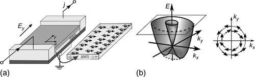
Assume the 2-D electron system is additionally confined along one of the in-plane directions to form a quasi-one-dimensional wire. When an external electric field is applied along the wire, the associated electric current – in the presence of spin–orbit interaction – leads to several spin-related effects. Similar phenomena are also generated by a temperature gradient along the wire. In this section we will consider one of such phenomena, that is, spin polarization of the electron gas induced by an electric field (current) and by a temperature gradient (thermocurrent). To describe this phenomenon theoretically, we consider a quasi-one-dimensional quantum wire shown schematically in Figure 18.1a. The electron gas is confined between the bottom (substrate) and upper (cover) layers, which generally are different. The induced Rashba spin–orbit interaction affects the spin orientation of electrons moving along the wire due to external electric field or temperature gradient and leads to an average spin polarization of conduction electrons, as shown schematically in Figure 18.1a. To present the theoretical approach to the problem of nonequilibrium spin polarization, we consider first the spin polarization induced by an external electric field. We show that the induced spin polarization of conduction electrons is oriented in the nanowire plane and is perpendicular to the electric field, see Figure 18.1a. Following we show in more detail how to calculate this nonequilibrium spin polarization.
18.2.1 Spin polarization induced by electric field
A simple model Hamiltonian of a 2-D electron gas confined in the x–y plane (plane of the quantum well) with the Rashba spin–orbit interaction can be written in the plane-wave basis as (Bychkov and Rashba, 1984)
where k is the two-dimensional wave vector, ɛk is the electron energy spectrum in the absence of Rashba coupling (kinetic term), g is the coupling constant of the Rashba spin–orbit interaction, and σi (i = x,y,z) are the Pauli matrices acting in the spin space. One should note that even though the spin–orbit interaction in quantum mechanics is a perturbative relativistic effect, the magnitude of the spin–orbit constant g in Eq. (18.1) can be relatively large in real materials. In the equilibrium situation (absence of external electric field) the electron spin is driven by the Rashba interaction to the orientation in the plane of 2-D electron gas and perpendicular to the electron momentum (perpendicular to the wave vector k), see Figure 18.1b. Accordingly, the average spin of the electron system in equilibrium is equal to zero for each subband separately.
For simplicity we assume the parabolic form of electron energy spectrum, ![]() , where m is an effective electron mass. This assumption is well justified for semiconducting quantum wells, but is less accurate for metallic ones. The approach described later can be generalized also to other systems, for instance to systems with linear spectrum, like in the case of a single-layer graphene (see the next section). When the system is confined along the x-direction to form a wire of width L, then the momentum component kx is quantized. We assume that the number of such quantum channels is relatively large, so the semiclassical approach to describe electron motion is justified.
, where m is an effective electron mass. This assumption is well justified for semiconducting quantum wells, but is less accurate for metallic ones. The approach described later can be generalized also to other systems, for instance to systems with linear spectrum, like in the case of a single-layer graphene (see the next section). When the system is confined along the x-direction to form a wire of width L, then the momentum component kx is quantized. We assume that the number of such quantum channels is relatively large, so the semiclassical approach to describe electron motion is justified.
When an electric field (bias voltage) is applied in the y-direction, an electric current flows along the wire with a certain current density jy, which is defined here as the current per unit width of the wire. Obviously, the system with a nonzero current is not in equilibrium. However, to calculate this current one does not necessarily needs to consider properties of the system out of equilibrium, at least for not too large currents. Instead, one can calculate the current–current correlation function of two current operators at equilibrium (Mahan, 2000), 〈[ ĵi(r, t), ĵj(r′, t′)]〉 for (i,j = x,y),1 which is related to the electric conductivity of the system. This method, known as the Kubo formalism for the conductivity, is very convenient for theoretical considerations, as it allows to stay within an equilibrium situation and describe material properties resulting from a small deviation of the system from the equilibrium (driven by electric field, for instance). Obviously, the Kubo method leads to the same results as the linear response approach to the electron and spin transport (Abrikosov et al., 1963; Mahan, 2000).
Using the Kubo formalism, one can calculate not only the charge current, but also a nonequilibrium part of magnetization, that is, the current-induced average spin polarization 〈si〉 (for i = x,y,z) of electrons in the system. This can be done by calculating the spin and electric current correlator, 〈[ŝi(r, t), ĵj(r′, t′)]〉, which describes the spin-density response to the charge-current perturbation. Note that the electron spin s is given by ![]() , where σ is the vector of Pauli matrices. From the theoretical point of view, to find the spin polarization one has to evaluate the corresponding Kubo diagram.
, where σ is the vector of Pauli matrices. From the theoretical point of view, to find the spin polarization one has to evaluate the corresponding Kubo diagram.
In the linear response regime the spin polarization driven by an electric field can be written as ![]() for i = x,y,z and j = x,y. In the zero-temperature limit and in the bubble approximation, the corresponding analytical formula for the linear magneto-electric coefficient pij is given by (Edelstein, 1990; Dyrdał et al., 2013)
for i = x,y,z and j = x,y. In the zero-temperature limit and in the bubble approximation, the corresponding analytical formula for the linear magneto-electric coefficient pij is given by (Edelstein, 1990; Dyrdał et al., 2013)

where G(k, ɛ) is the Green function corresponding to the Hamiltonian (18.1), vj is the jth component of the electron velocity, − e is the electron charge (e > 0), and ![]() . Apart from this, ω is the frequency of the driving electric field. The Green function G(k, ɛ) has the form
. Apart from this, ω is the frequency of the driving electric field. The Green function G(k, ɛ) has the form

where μ is the chemical potential of electrons in equilibrium, whereas δ is a small parameter that can be associated with the electron momentum relaxation time τk as ![]() . A small term, iδ sgnɛ, in the nominator of the Green function has been omitted in Eq. (18.3). The electron energy ɛ is measured here from the chemical potential. In the assumed bubble approximation, the electron scattering is included only in the Green function through the relaxation time. More detailed description requires including vertex correction, which modifies the spin polarization as described later. This approach can be generalized to a nonzero temperature by rewriting the formula (18.2) in terms of the Matsubara Green functions (Dyrdał et al., 2013). Technical details of this formalism will not be presented here.
. A small term, iδ sgnɛ, in the nominator of the Green function has been omitted in Eq. (18.3). The electron energy ɛ is measured here from the chemical potential. In the assumed bubble approximation, the electron scattering is included only in the Green function through the relaxation time. More detailed description requires including vertex correction, which modifies the spin polarization as described later. This approach can be generalized to a nonzero temperature by rewriting the formula (18.2) in terms of the Matsubara Green functions (Dyrdał et al., 2013). Technical details of this formalism will not be presented here.
In a general case of non-zero temperature, the nonvanishing component (for electric field along the y axis) of the current-induced spin polarization of conduction electrons can be written as (Dyrdał et al., 2013)

where ![]() describe the two electronic subbands with the effects of Rashba spin–orbit interaction included, whereas f′(ɛ) is the first derivative of the Fermi–Dirac distribution function with respect to the energy ɛ. Dispersion relations corresponding to the electronic bands
describe the two electronic subbands with the effects of Rashba spin–orbit interaction included, whereas f′(ɛ) is the first derivative of the Fermi–Dirac distribution function with respect to the energy ɛ. Dispersion relations corresponding to the electronic bands ![]() are shown in Figure 18.1b. Due to the term linear in k, which follows from the Rashba interaction, minimum energy in the lower subband,
are shown in Figure 18.1b. Due to the term linear in k, which follows from the Rashba interaction, minimum energy in the lower subband, ![]() , is shifted away from k = 0. When the Rashba spin–orbit coupling is small, the preceding formula (18.4) can be rewritten in a more transparent form, which is linear in the spin–orbit parameter,
, is shifted away from k = 0. When the Rashba spin–orbit coupling is small, the preceding formula (18.4) can be rewritten in a more transparent form, which is linear in the spin–orbit parameter,

where f″(ɛ) is the second derivative of the distribution function.
The preceding expressions clearly show that the nonequilibrium spin polarization vanishes in the absence of spin–orbit coupling, ![]() for i = x,y,z when
for i = x,y,z when ![]() . Apart from this, only one component of the field-induced spin polarization is nonzero for
. Apart from this, only one component of the field-induced spin polarization is nonzero for ![]() , that is, the component oriented in the plane of the electron gas and perpendicular to the electric field. In the limit of low temperatures,
, that is, the component oriented in the plane of the electron gas and perpendicular to the electric field. In the limit of low temperatures, ![]() (with kB being the Boltzmann constant), the preceding equations can be further simplified. Assuming constant, that is, independent of energy and momentum relaxation time,
(with kB being the Boltzmann constant), the preceding equations can be further simplified. Assuming constant, that is, independent of energy and momentum relaxation time, ![]() , one finds a simple formula for the spin polarization. This polarization depends on the chemical potential and can be written as
, one finds a simple formula for the spin polarization. This polarization depends on the chemical potential and can be written as
and

where n in Eq. (18.7) is the electron density corresponding to the chemical potential μ ![]() , and n * is the electron density corresponding to
, and n * is the electron density corresponding to ![]() . In the preceding formulas we introduced a prefactor κ, which takes into account the vertex correction,
. In the preceding formulas we introduced a prefactor κ, which takes into account the vertex correction, ![]() . Thus, in the bubble approximation one has to set κ = 1 in the preceding equations. In turn, the vertex correction calculated in the ladder approximation gives κ = 2. Expressions corresponding to Eq. (18.6) were derived first by Edelstein (1990), Aronov and Lyanda-Geller (1989), and Aronov et al. (1991) and also confirmed by other calculations (Liu et al., 2008; Gorini et al., 2008; Wang et al., 2009; Schwab et al., 2010; Golub and Ivchenko, 2011).
. Thus, in the bubble approximation one has to set κ = 1 in the preceding equations. In turn, the vertex correction calculated in the ladder approximation gives κ = 2. Expressions corresponding to Eq. (18.6) were derived first by Edelstein (1990), Aronov and Lyanda-Geller (1989), and Aronov et al. (1991) and also confirmed by other calculations (Liu et al., 2008; Gorini et al., 2008; Wang et al., 2009; Schwab et al., 2010; Golub and Ivchenko, 2011).
The spin polarization generally depends on the chemical potential μ (electron concentration) and also on temperature. This dependence is shown in Figure 18.2, where the spin polarization including the vertex correction is normalized to τeEy. The chemical potential varies there down to values below the band edge. Note, this band edge is determined by the minimum energy in the subband ![]() . When the chemical potential is below the band edge, the subbands are populated only for nonzero temperatures because at zero temperature the electrons are localized at donors.
. When the chemical potential is below the band edge, the subbands are populated only for nonzero temperatures because at zero temperature the electrons are localized at donors.
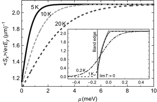
 ) for different temperatures, calculated for g = 2 × 10− 2 meV μm, and m = 0.05m0, where m0 is the free electron mass. The vertex correction is included. The inset shows the low-temperature spin polarization in the regime of small (negative and positive) chemical potentials.
The spin polarization in a particular subband is driven by a simultaneous action of electric and Rashba fields. When an electron is accelerated by the electric field, its wavevector component parallel to the field becomes changed, that is, the wavevector k and the associated Rashba field change their orientations. The electron spin starts then to precess around the new orientation of the Rashba field, which on average generates a spin polarization of electrons in a particular subband. The average spin polarizations in the two subbands have opposite orientations, but their magnitudes are nonequivalent due to different densities of states corresponding to these subbands. As a result, a nonzero net spin polarization appears in the system.
For a nonzero temperature, the spin polarization increases with increasing μ and saturates at a constant value when μ is sufficiently large. For T = 0, this dependence is especially simple. When the Fermi level is in both electronic subbands, which takes place for positive μ, the spin polarization is then constant. For negative μ, when the Fermi level is in the subband ![]() only, the spin polarization decreases with decreasing μ and vanishes at the band edge. For higher temperatures, T > 0, the spin polarization decreases with increasing temperature for μ > 0. When the Fermi level is in the subband
only, the spin polarization decreases with decreasing μ and vanishes at the band edge. For higher temperatures, T > 0, the spin polarization decreases with increasing temperature for μ > 0. When the Fermi level is in the subband ![]() only, μ < 0, the tendency is opposite, and the spin polarization increases with increasing temperature. Moreover, spin polarization is then nonzero also for μ below the band edge due to thermal excitation of electrons. This behavior of the field-induced spin polarization is shown explicitly in Figure 18.2.
only, μ < 0, the tendency is opposite, and the spin polarization increases with increasing temperature. Moreover, spin polarization is then nonzero also for μ below the band edge due to thermal excitation of electrons. This behavior of the field-induced spin polarization is shown explicitly in Figure 18.2.
The approach described earlier takes into account momentum relaxation processes, whereas energy relaxation is not included explicitly. Such processes were considered by Golub and Ivchenko (2011), who used the Boltzmann kinetic equation to calculate the current-induced spin polarization. The energy relaxation was shown to play an important role, when the corresponding relaxation time is shorter than the momentum and spin relaxation times and leads to an additional factor of 2 in the formula for the induced spin density (Golub and Ivchenko, 2011). This factor may be effectively included into the prefactor κ, which can be then treated as the factor that includes the vertex correction and the correction due to energy relaxation. Physical mechanism of the current-induced spin polarization, and also of the inverse effect—current generation by spin polarization—was described in detail in a review article by Ivchenko and Ganichev (2008) and by Ganichev et al. (2002).
18.2.2 Thermally induced spin polarization
Effects similar to those generated by an electric field can also appear due to a temperature gradient along the wire (Wang and Pang, 2010). Theoretical description of the thermally induced spin polarization, in a certain sense, is similar to that in the case of electric field, though there is an important difference. Instead of the vector potential describing external electric field, one needs to introduce an auxiliary vector potential, which is associated with the heat current density operator, ![]() , and which takes into account the thermal gradient as the driving force (Luttinger, 1964; Strinati and Castellani, 1987). Here,
, and which takes into account the thermal gradient as the driving force (Luttinger, 1964; Strinati and Castellani, 1987). Here, ![]() is defined as
is defined as ![]() for any two operators
for any two operators ![]() and
and ![]() . One can formally develop a perturbation scheme, which is similar to that for electric field as the driving force. The perturbation now is given as
. One can formally develop a perturbation scheme, which is similar to that for electric field as the driving force. The perturbation now is given as ![]() instead of
instead of ![]() . The auxiliary vector potential AQ (ω) can be identified as (i/ω)
. The auxiliary vector potential AQ (ω) can be identified as (i/ω) ![]() . According to the discussion presented in the previous subsection, the correlation function that describes the effect of thermally induced spin polarization has the form
. According to the discussion presented in the previous subsection, the correlation function that describes the effect of thermally induced spin polarization has the form ![]() .
.
The thermally induced linear spin polarization can be written as ![]() , where ξi,j is the corresponding magneto-thermoelectric coefficient. In the low-temperature regime one can simplify the problem and take the zero-temperature Green functions. In the bubble approximation ξi,j takes then the form
, where ξi,j is the corresponding magneto-thermoelectric coefficient. In the low-temperature regime one can simplify the problem and take the zero-temperature Green functions. In the bubble approximation ξi,j takes then the form

In a general case, however, one needs to use the finite-temperature formalism based on the Matsubara Green functions (Dyrdał et al., 2013). Assume the temperature gradient is along the wire (axis y), ![]() , whereas the other components of the gradient disappear. Using the general formulation based on the Matsubara Green functions, one finds that the only nonzero component of the spin polarization is perpendicular to the temperature gradient and is oriented in the plane of electron gas, exactly like in the case of the field-induced spin polarization. The corresponding formula takes the form (Dyrdał et al., 2013)
, whereas the other components of the gradient disappear. Using the general formulation based on the Matsubara Green functions, one finds that the only nonzero component of the spin polarization is perpendicular to the temperature gradient and is oriented in the plane of electron gas, exactly like in the case of the field-induced spin polarization. The corresponding formula takes the form (Dyrdał et al., 2013)

where all other parameters have the same meaning as in Section 18.2.1. Note that the preceding formula is very similar to Eq. (18.4). In the limit of small spin–orbit interaction, one can take into account only the leading term (linear in g) and write the thermoelectric spin polarization in the form,

which corresponds to Eq. (18.5) in the case of the field-induced polarization.
Equation (18.9) allows to find simple analytical formulas for the thermally induced spin polarization in the limit of low temperatures. In the case of positive chemical potentials, μ > 0, when both electron subbands are occupied with electrons at T = 0, one finds the dominant contribution (linear in g) in the form,

where, for simplicity, the relaxation time is assumed to be constant. In turn, when μ < 0, that is, when only the subband ![]() is populated at T = 0, the dominant contribution to the spin polarization is given by the formula
is populated at T = 0, the dominant contribution to the spin polarization is given by the formula

where n and n* have the same meaning as in Eqs. (18.6) and (18.7). As before, κ = 1 in the bubble approximation, and κ = 2 when the vertex correction is included.
Variation of the temperature-gradient-induced spin polarization with the chemical potential μ is shown in Figure 18.3. The spin polarization, including the vertex correction, is normalized there to ![]() , and different curves correspond to different temperatures. The main figure shows the range of positive chemical potential and for higher temperatures, whereas the inset shows the low-temperature spin polarization for chemical potentials in the vicinity of the band edge (negative μ). Let us consider first the low T limit of the spin polarization, given by Eqs. (18.11) and (18.12). For positive μ, the spin polarization decreases linearly with decreasing μ and turns to zero at
, and different curves correspond to different temperatures. The main figure shows the range of positive chemical potential and for higher temperatures, whereas the inset shows the low-temperature spin polarization for chemical potentials in the vicinity of the band edge (negative μ). Let us consider first the low T limit of the spin polarization, given by Eqs. (18.11) and (18.12). For positive μ, the spin polarization decreases linearly with decreasing μ and turns to zero at ![]() . Then, it becomes negative for μ < 0 and decreases with decreasing chemical potential until μ reaches the band edge. Behavior for slightly higher temperatures is similar, except that the spin polarization reaches a minimum close to the band edge and then increases toward zero for chemical potentials well below the band edge. Thus, the spin polarization at low temperatures changes sign at
. Then, it becomes negative for μ < 0 and decreases with decreasing chemical potential until μ reaches the band edge. Behavior for slightly higher temperatures is similar, except that the spin polarization reaches a minimum close to the band edge and then increases toward zero for chemical potentials well below the band edge. Thus, the spin polarization at low temperatures changes sign at ![]() . For slightly higher temperatures, the point, where the spin polarization changes sign moves toward negative values of μ. For sufficiently high temperatures, the spin polarization does not change sign in the range of μ shown in Figure 18.3.
. For slightly higher temperatures, the point, where the spin polarization changes sign moves toward negative values of μ. For sufficiently high temperatures, the spin polarization does not change sign in the range of μ shown in Figure 18.3.

Physical origin of the thermally induced spin polarization is similar to that for the current-induced polarization. There is, however, an important qualitative difference. Now, the polarization is a result of a nonzero balance of spin flow associated with electrons flowing from the higher and lower temperatures and not due to the rotation of electron spin.
18.3 Nonequilibrium spin polarization in graphene
In this section we consider a nonequilibrium spin polarization in another 2-D system, that is, in graphene – an atomic monolayer of carbon atoms. Due to its outstanding properties, graphene is one of the most attractive 2-D electron systems, and is an excellent material for applications in future nanoelectronics and spin electronics—similarly as other strictly 2-D crystals like silicene (atomic monolayer of silicon atoms), for instance. This is because these 2-D materials have unique transport properties, which follow from their specific electronic band structure. The intrinsic spin–orbit interaction in graphene is negligibly small. However, the Rashba spin–orbit coupling can be significant for graphene on a substrate, and strength of this coupling depends on the material used as the substrate. In the following section we consider a graphene ribbon deposited on a substrate, which generates the Rashba spin–orbit interaction, see Figure 18.4. When an electric field (bias voltage) is applied along the ribbon, the associated current generates spin polarization, similar to the case of 2-D electron gas. To calculate the induced spin polarization, one can use the method described in Section 18.2.

18.3.1 Electric-field-induced spin polarization
For simplicity, we limit our discussion to the situation, where transport properties are determined by electrons in the vicinity of the Dirac points, that is, where the low-energy electrons are described by the relativistic quantum mechanics. The corresponding Hamiltonian for electrons in the vicinity of the Dirac point K takes then the form (Kane and Mele, 2005)
where ![]() , with v being the electron velocity in graphene, whereas ςx and ςy are the Pauli matrices acting in the space of the two, A and B, sublattices in graphene (Castro Neto et al., 2009; Katsnelson, 2012). The parameter η is connected with the hopping integral t between the nearest neighbors via the formula
, with v being the electron velocity in graphene, whereas ςx and ςy are the Pauli matrices acting in the space of the two, A and B, sublattices in graphene (Castro Neto et al., 2009; Katsnelson, 2012). The parameter η is connected with the hopping integral t between the nearest neighbors via the formula ![]() where a0 is the distance between nearest-neighbor carbon atoms. The second term in Eq. (18.13) stands for the Rashba spin–orbit interaction, with g being the relevant coupling parameter. The electronic spectrum corresponding to the Hamiltonian (18.13) consists of the following four energy bands:
where a0 is the distance between nearest-neighbor carbon atoms. The second term in Eq. (18.13) stands for the Rashba spin–orbit interaction, with g being the relevant coupling parameter. The electronic spectrum corresponding to the Hamiltonian (18.13) consists of the following four energy bands:
This spectrum is parabolic in the vicinity of the Dirac point (corresponding to ![]() ). In the absence of Rashba interaction, the energy spectrum has the standard form characteristic of Dirac cones, with the linear dependence on k,
). In the absence of Rashba interaction, the energy spectrum has the standard form characteristic of Dirac cones, with the linear dependence on k, ![]() (Castro Neto et al., 2009; Katsnelson, 2012). Note that the Rashba coupling lifts the double degeneracy of the Dirac cones and also removes the linear dispersion relations.
(Castro Neto et al., 2009; Katsnelson, 2012). Note that the Rashba coupling lifts the double degeneracy of the Dirac cones and also removes the linear dispersion relations.
The spin polarization induced by current flowing along the wire (axis y) due to an external electric field can be found by the same method as in Section 18.2. The formula (18.2) for the magneto-electric coefficient is still applicable, but the electron Green function corresponds now to the Hamiltonian (18.13) and therefore has a different form (Dyrdał et al., 2014). We restrict the following discussion to the zero-temperature limit, T = 0. When the chemical potential is relatively small (the chemical potential is measured from the Dirac point corresponding to the energy ![]() ),
), ![]() , the spin polarization 〈sx〉 in the bubble approximation (including contribution from the second Dirac point, K′) is given by the formula
, the spin polarization 〈sx〉 in the bubble approximation (including contribution from the second Dirac point, K′) is given by the formula

where the plus and minus signs correspond to the case of ![]() and
and ![]() , respectively. If the chemical potential is relatively large,
, respectively. If the chemical potential is relatively large, ![]() , the corresponding formula for the induced spin density takes the form
, the corresponding formula for the induced spin density takes the form

When the vertex correction is included, an additional factor may appear in the preceding formulas, similarly as in the case of 2-D electron gas.
The dependence of spin polarization on the spin–orbit coupling constant g as well as on the chemical potential μ is now more complex than in the case of a 2-D electron gas considered in Section 18.2. The formulas (18.15) and (18.16) reveal two features of the current-induced spin polarization in graphene, which follow from its specific electronic structure. First, the spin polarization vanishes for the Fermi level at the Dirac point, μ = 0. This results from a peculiar behavior of the spin associated with the eigenstates, including Rashba coupling – the expectation value of the electron spin in the eigenstate corresponding to the Dirac point, k = 0, vanishes (Rashba, 2009). Second, the spin polarization changes sign when the Fermi level passes through the Dirac point. This behavior is different from that observed in the 2-D electron gas, where the spin polarization does not change sign. Both features mentioned earlier are clearly visible in Figure 18.5, which shows a variation of the spin polarization with the chemical potential for constant Rashba parameters. When the absolute value of the chemical potential is remarkably larger than the parameter of Rashba coupling, the magnitude of spin polarization increases with g and is roughly independent of μ. In turn, when ![]() is smaller than the Rashba parameter, the spin polarization is roughly independent of g, but varies linearly with the chemical potential μ. Between these two limiting situations, amplitude of the spin polarization reaches a maximum value when |μ| = 2g.
is smaller than the Rashba parameter, the spin polarization is roughly independent of g, but varies linearly with the chemical potential μ. Between these two limiting situations, amplitude of the spin polarization reaches a maximum value when |μ| = 2g.

Physical mechanism of the field-induced spin polarization in graphene is similar to that in the case of 2-D electron gas. However, the system has now features that distinguish it from the 2-D electron gas and that are related to specific properties of the electron eigenfunctions in graphene with Rashba coupling. The expectation value of electron spin in an eigenstate is oriented in the graphene plane and is normal to the corresponding wave vector k, similar to the 2-D electron gas. However, unlike the 2-D electron gas, the absolute value of the spin is not constant but depends on k (Rashba, 2009; Liu and Chang, 2009). Orientation of the electron spin corresponding to a particular k depends on the electron band. This orientation is the same for the bands that touch at μ = 0 and is opposite to the spin orientation in the other two bands. Accordingly, when the chemical potential obeys the condition |μ| < 2g, only one electron band contributes to the spin polarization. When, however, |μ| > 2g, another electron band contributes, but this contribution is opposite due to the opposite spin orientation in the corresponding eigenstates, so the absolute value of spin polarization becomes reduced, as clearly visible in Figure 18.5. Moreover, spin polarization changes sign at μ = 0. Though the spin orientation is symmetrical with respect to the plane μ = 0, the current-induced spin polarization is asymmetrical. This also holds for the contribution from the second Dirac point, K′. The spin orientation attributed to the electron bands is the same as in the K point (Rashba, 2009), which makes both contributions equivalent.
18.3.2 Thermally induced spin polarization
As in the case of two-dimensional electron gas considered in the preceding section, the spin polarization of graphene can be driven by a temperature gradient as well, and the thermally induced spin polarization can be calculated using the method described in Section 18.2.2. Following this approach, the thermally induced spin polarization can be expressed as an equilibrium spin-density–thermal-flux correlator. This leads again to Eq. (18.8), with G(k, ɛ) being the Green function corresponding to the Hamiltonian of graphene with the Rashba spin–orbit coupling included. However, after integrating over the energy ɛ and calculating the trace in the spin and sublattice spaces, one finds that the temperature-gradient-induced spin polarization in graphene is equal zero, ![]() , when the relaxation time is independent of the wavevector and subband index n,
, when the relaxation time is independent of the wavevector and subband index n, ![]() .
.
To have a nonzero spin density, one needs to take into account variation of the electron relaxation time τnk with the electron momentum and subband index. Such calculations have been performed in terms of the exact T-matrix method for scattering of electrons from a short-range impurity potential V0 (Inglot and Dugaev, 2011). The corresponding numerical results for the spin polarization 〈sx〉 as a function of the chemical potential μ are presented in Figure 18.6 for different values of the impurity potential V0 and for a typical value of the Rashba parameter. The parameter Vc in Figure 18.6 is defined as ![]() .
.

 , g = 6.5 meV, t = 3 eV, and a0 = 1.4 Å. The normalization constant τ0 is set equal to
  , whereas the parameter Vc is defined as
  .
.Figure 18.6 shows that the spin polarization induced by a temperature gradient has different signs for positive and negative μ, similar to the case of current-induced spin polarization. For positive chemical potential μ, the spin polarization is negative, whereas for negative μ the spin polarization is positive. Moreover, the magnitude of spin polarization depends on the impurity scattering potential. Interestingly, there is now some asymmetry in the magnitude of spin polarization for negative and positive μ. This asymmetry appears due to impurity potential, which brakes the electron-hole symmetry. There are local maxima in the absolute value of the spin polarization, which appear near the band edges, ![]() . Such maxima also appear in the current-induced spin polarization, see Figure 18.5. One should also note that the absolute magnitude of the spin polarization for
. Such maxima also appear in the current-induced spin polarization, see Figure 18.5. One should also note that the absolute magnitude of the spin polarization for ![]() is remarkably smaller than that for
is remarkably smaller than that for ![]() .
.
18.4 Thermally induced spin-polarized current
In the preceding two sections we have considered static spin polarization induced by electric field and temperature gradient in the presence of spin–orbit coupling. However, electric field (and temperature gradient) can also lead to spin-dependent kinetic phenomena, like spin-polarized currents. Generally, electric current in ferromagnetic metals and semiconductors is intrinsically spin-polarized, and therefore charge current is accompanied by a spin current flowing along the same direction. This is an intrinsic property of ferromagnetic conductors, and the spin current is not associated with any spin–orbit interaction. The situation is different when the system is nonmagnetic. Charge current in such a material is not accompanied by any spin current flowing in the same direction. However, when spin–orbit interaction is present in the system, electric current flowing along the wire generates a pure spin current flowing perpendicularly to the electric field (or spin accumulation at the wire edges). This phenomenon is known as the spin Hall effect (Dyakonov and Khaetskii, 2008). The spin current is then a response to the charge current, but both currents are perpendicular to each other. This happens, for instance, in wires based on 2-D electron gas or graphene with Rashba spin–orbit interaction. Moreover, the spin–orbit interaction may be generally either of intrinsic (inherent property of a material) or extrinsic (due to impurities or substrate) origins. There is already a very rich literature on the field-induced spin-polarized currents, so in the following we focus only on the thermally induced spin polarized currents.
Because current in a magnetic system is inherently spin polarized, a temperature gradient in such a system generates charge current (via the Seebeck effect), which is spin polarized as well. In other words, a temperature gradient generates both charge and spin currents flowing along the wire. When the wire is nonmagnetic but includes spin–orbit interactions, then in addition to the charge current flowing along the wire due to the Seebeck effect, the thermal gradient generates also a pure spin current flowing perpendicularly to the temperature gradient. This phenomenon is referred to as the thermally induced spin Hall effect or the spin Nernst effect.
From the theoretical side, the electric current induced by the temperature gradient can be calculated from the correlation function ![]() , where
, where ![]() is the operator of heat flux defined in Section 18.2.2. By introducing the spin-current operator
is the operator of heat flux defined in Section 18.2.2. By introducing the spin-current operator ![]() , one can also consider the temperature-gradient-induced spin current. The relevant correlation function is then
, one can also consider the temperature-gradient-induced spin current. The relevant correlation function is then ![]() . In the low-temperature regime, the corresponding Kubo formula for the thermoelectrically induced spin current leads to the following thermoelectric coefficient:
. In the low-temperature regime, the corresponding Kubo formula for the thermoelectrically induced spin current leads to the following thermoelectric coefficient:

where ![]() describes the spin current induced by a temperature gradient and is defined by the relation
describes the spin current induced by a temperature gradient and is defined by the relation ![]() . In a more general case one needs to apply the Matsubara finite-temperature approach. The preceding formula for
. In a more general case one needs to apply the Matsubara finite-temperature approach. The preceding formula for ![]() includes both the longitudinal and transverse effects. The spin current due to Seebeck effect corresponds to the coefficient
includes both the longitudinal and transverse effects. The spin current due to Seebeck effect corresponds to the coefficient ![]() , whereas that due to the spin Nernst effect corresponds to
, whereas that due to the spin Nernst effect corresponds to ![]() for k ≠ j. In the following section we describe briefly both effects.
for k ≠ j. In the following section we describe briefly both effects.
18.4.1 Seebeck and spin Seebeck effects
An important property of ferromagnetic conducting systems, which is responsible for spin currents, is the existence of two nonequivalent and well-defined spin channels for electronic transport. As a result, the electrochemical potentials for spin-up and spin-down electrons can be different in the vicinity of an interface between ferromagnetic and nonmagnetic materials, which appears as a spin accumulation at the interface (Valet and Fert, 1993). Following this, the difference in electrochemical potentials of the two electrodes in the spin-σ channel, δVσ, can be written as δVσ = δV ± δVS, with the upper (lower) sign corresponding to σ = ↑(↓). Here, δV is the electrical voltage, whereas δVS stands for the spin voltage.
Thus, when a temperature gradient along the wire is nonzero, both spin and charge currents can flow in the system. These currents can be calculated from the general formalism based on the Kubo formula described earlier. However, we will not present results on the thermoelectrically induced currents, but instead describe some general thermoelectric parameters that describe thermoelectric response of the system, that is, thermopower and spin thermopower. Assuming zero charge current, I = 0, one finds then a nonzero voltage δV and spin voltage δVS in an electrically open system in the presence of temperature gradient. The former effect is known as the Seebeck effect and is described by the corresponding thermopower S (Hatami et al., 2009; Dubi and Di Ventra, 2009; Bauer et al., 2012),

The latter effect, in turn, is the spin Seebeck effect, which is a spin analog of the Seebeck effect and is described by the spin thermopower SS (Uchida et al., 2012; Bauer et al., 2012; Adachi et al., 2013),

The spin Seebeck effect was studied theoretically in a variety of systems, including molecular junctions, quantum dots, planar magnetic junctions, spin valves, and others. It was also observed experimentally (e.g., in a ferromagnetic slab; Uchida et al., 2010). The spin Seebeck effect is a general phenomenon associated with different spin channels and is observable when size of the system is of the order of spin diffusion or spin coherence length. It can also appear in wires of 2-D systems like graphene, silicene, and other 2-D graphene-like crystals. Electronic structure and magnetic properties of such wires depend on structural properties of the wire edges. When the edges are of the zigzag type, the wires reveal edge magnetism, and the magnetic moments at the two edges in the ground state are antiparallel. By a specific functionalization of the edges, one can induce ferromagnetic configuration in the ground state. This, in turn, leads to spin-dependent electronic structure and spin-dependent transport properties. As a consequence, the nonequivalence of the spin channels gives rise to the spin Seebeck effect (Zberecki et al., 2014). The corresponding spin thermopower depends on the position of the Fermi level, which in such systems can be tuned by an external gate voltage. Thus, temperature gradient along micro- or nano-wires of graphene and other graphene-like 2-D crystals can generate both charge and spin currents flowing along the wire (parallel to the temperature gradient).
18.4.2 Spin Nernst effect
As mentioned earlier, the temperature gradient along a wire may also generate transverse currents in systems with spin–orbit interactions. When the system is magnetized and includes spin–orbit interactions (e.g., due to impurities or due to a substrate), the temperature gradient generates transverse charge and spin currents (i.e., a spin-polarized current). This effect is similar to the anomalous Hall effect, where transverse spin-polarized current is generated by an electric field (or voltage) along the wire. In turn, when a system is nonmagnetic, the temperature gradient along the wire in the presence of spin–orbit interaction leads to a pure transverse spin current (so-called spin Nernst effect). The spin Nernst effect can be thus used to generate a pure spin current that is not accompanied by a charge current flowing in the same direction (the charge thermo-current is perpendicular to the spin current). The spin Nernst conductivity ![]() can be defined as
can be defined as
for i = x,y,z and j,k = x,y with j ≠ k.
It has been shown that the low-temperature spin Nernst conductivity and the zero-temperature spin Hall conductivity ![]() are not independent and obey some general relation (Chuu et al., 2010; Lie and Xie, 2010),
are not independent and obey some general relation (Chuu et al., 2010; Lie and Xie, 2010),

which is a spin analog of the Mott's relation for charge transport. Here the derivative of the spin Hall conductivity with respect to the energy ɛ is taken at the Fermi level μ.
The spin Nernst effect was studied theoretically (Lie and Xie, 2010; Tauber et al., 2012; Rothe et al., 2012; Dyrdał and Barnaś, 2012; Lyapilin, 2013; Borge et al., 2013) mainly in the low-temperature regime. Its behavior depends on the nature of spin–orbit interaction taken into account and is correlated with the zero-temperature spin Hall effect. For instance, when the spin–orbit interaction is of the Rashba type, the spin Hall conductivity of a 2-D electron gas acquires a universal value (Sinova et al., 2004). In turn, the Rashba interaction in graphene does not lead to a universal spin Hall conductance, and such a universal conductance in graphene can appear in the presence of intrinsic spin–orbit interaction when the Fermi level is in the gap created by the spin–orbit interaction (Kane and Mele, 2005). The spin Nernst conductivity in the low-temperature regime, however, is not universal and is correlated with the spin Hall conductivity according to Eq. (18.21). For instance, the spin Hall and spin Nernst conductivities of graphene due to Rashba spin–orbit interactions are shown in Figure 18.7. Neither the spin Hall conductivity nor the spin Nernst conductivity are then universal. Interestingly, the spin Nernst conductivity tends to zero when |μ| ![]() 2g (Dyrdał and Barnaś, 2012).
2g (Dyrdał and Barnaś, 2012).

The results presented in Figure 18.7 are for a clean system, that is, a system with no impurities and other structural defects. However, it is known that impurities have a significant influence on the spin Hall effect and can even suppress the effect. Accordingly, the impurity scattering can also significantly modify the spin Nernst conductivity.
18.5 Thermoelectrically induced spin torque
The spin polarization and spin currents discussed in Sections 18.2–18.4 may generate a torque exerted on magnetization and thus may be used to control the state of a magnetic moment. Accordingly, the mechanisms of spin torque generation (and thus of the control of magnetic moments) can be classified into two groups, which are closely related to the spin currents and spin polarization, respectively. The first group relies on the transfer of angular momentum from spin current to magnetization. This spin transfer (usually due to exchange interaction) appears in systems with spatially nonuniform magnetization. The absorbed spin current creates then a torque (called spin-transfer torque), which leads to various physical effects, like switching orientation of magnetic moments (Katine et al., 2000), excitation of stationary precessions supported by current (Boulle et al., 2007), domain wall shifts (Parkin et al., 2008), and others. The second class of mechanisms leading to manipulation of magnetic moments relies on an effective magnetic field due to spin–orbit interaction. For example, when a thin magnetic film is deposited on a substrate, which creates a spin–orbit coupling of Rashba type, the current/thermocurrent generates a nonzero effective magnetic field due to Rashba coupling, and this field can switch orientation of the magnetic moment (Manchon and Zhang, 2008). In other words, the electric field or temperature gradient in the presence of spin–orbit interaction induce a spin polarization, and the induced spin polarization modifies the local magnetization (Kurebayashi et al., 2014). This modification may be either direct or indirect (via exchange coupling). The induced spin polarization then gives rise to a spin torque acting on the magnetization, and in appropriate conditions the induced spin torque can change orientation of the local magnetization. It is worth noting that according to our definition, the torque due to spin current generated by spin–orbit interaction via the spin Hall or spin Nernst effects is included to the first class of the spin torque mechanisms. The previously described mechanisms apply to both thermal and field control of magnetic moments. In the case of thermal control, one needs a temperature gradient as the driving force. In fact, many mechanisms leading to electric control are also applicable to thermal control of magnetic moments. Later in this section we describe only two of them, that is, thermal spin-transfer torque and thermal spin–orbit torque.
Before doing this, however, it is also worthwhile to note, that the aforementioned two classes of physical mechanisms leading to control of magnetic moments are not the only ones. For instance, in ferromagnetic semiconductors one can electrically control the density of holes in valance bands, and a change in the hole density can affect magnetic anisotropy. The change in magnetic anisotropy, in turn, has an influence on the magnetic state of the system and may lead to reorientation of the moment (Chiba et al., 2008). Another type of electrical manipulation of magnetic moments occurs in magnetic tunnel junctions, where a voltage applied to the junction with a sufficiently thick barrier to suppress current leads to a change in magnetic anisotropy (Nozaki et al., 2012).
18.5.1 Thermally induced spin-transfer torque
Assume that a wire of 2-D material consists of three nonmagnetic and two magnetic parts, as shown schematically in Figure 18.8. The central and external parts of the wire are nonmagnetic, whereas the two narrow stripes of the wire are magnetic. The magnetic parts (also referred to as polarizer and analyzer) can be achieved, for instance, due to contact with a ferromagnetic substrate. When a temperature gradient is along the wire, then a thermally induced spin-polarized current, that is, charge current accompanied by a spin current, can flow along the wire. When magnetic moments of the two ferromagnetic parts are not collinear, then the component of spin current perpendicular to the magnetization of a particular magnetic part is absorbed by the corresponding magnetization. This corresponds to a spin torque exerted on the magnetization. Such absorption of spin current takes place essentially in a very narrow region at the contact between the nonmagnetic and magnetic parts. In well-conducting materials, the transfer component of spin current disappears in the magnetic systems, usually on the distance of a few atomic spacings. The spin-transfer torque τ per unit width of the wire, exerted on a mono-domain magnetic part in such a 2-D spin valve, can be thus calculated as
where ![]() and
and ![]() are the normal to the magnetization components of the thermally induced spin current at the left and right interfaces of a magnetic stripe, calculated on the nonmagnetic sides of this stripe.
are the normal to the magnetization components of the thermally induced spin current at the left and right interfaces of a magnetic stripe, calculated on the nonmagnetic sides of this stripe.

The torque is usually decomposed into two components: one in the plane formed by the two magnetic moments of the spin-valve, and the other one normal to this plane (Barnas et al., 2005),
where SF and SP are the unit vectors along the spin polarization of the free and polarizing magnetic parts, respectively, whereas a and b are some parameters that depend on the system and transport regime. The first term is in the plane formed by magnetic moments of the two magnetic films and is denoted by ![]() in Figure 18.8, whereas the second component is perpendicular to this layer and is denoted as
in Figure 18.8, whereas the second component is perpendicular to this layer and is denoted as ![]() in Figure 18.8.
in Figure 18.8.
This spin-transfer torque may excite magnetic components of the system and, for instance, may lead to magnetic switching of the spin valve between parallel and antiparallel magnetic configurations. Dynamics of the switching is well described by the macroscopic Landau–Lifshitz–Gilbert equation, which in addition to the torque due to effective magnetic field and the Gilbert damping, also includes the spin-transfer torque. Indeed, such a thermally induced spin-transfer torque was observed experimentally (Yu et al., 2010) in a metallic nanowire including thin layers of a magnetic metal separated by a thin layer of a nonmagnetic metal and attached to two nonmagnetic electrodes.
18.5.2 Thermally induced spin–orbit torque
Consider now the spin torque due to thermally induced spin polarization. When a system is magnetic, the thermally induced spin polarization can modify its magnetic state. Thus, the main task now is to find the thermally induced spin polarization of a magnetized electron system. Consider, for example, a magnetized nanowire of a 2-D electron gas. Hamiltonian of such a system is like that in Eq. (18.1), with an additional term associated with exchange interaction between conduction electrons of the 2-D electron gas and magnetization,
where J is the exchange coupling constant, and M is the magnetization.
Assume, for simplicity, that the magnetization is perpendicular to the plane of 2-D electron gas. Following the same procedure as in Section 18.2.2, one can calculate spin polarization induced by a temperature gradient along the wire (axis y). Now, the induced spin polarization has not only the in-plane component normal to the temperature gradient (x-component), but also the component parallel to the thermal gradient. The dominant term in the x component at low temperatures is that calculated in Section 18.2.2 and given by Eq. (18.11) for positive chemical potential. The component along the axis y (i.e., along the temperature gradient) is proportional to ![]() and to the exchange energy JM,
and to the exchange energy JM, ![]() . Obviously, this component vanishes when the electron gas is nonmagnetic.
. Obviously, this component vanishes when the electron gas is nonmagnetic.
The induced spin polarization s is coupled to the magnetization M via the exchange interaction, ![]() , where
, where ![]() is related to J in Eq. (18.24). This interaction leads to a torque exerted on the magnetization M, which may be written as
is related to J in Eq. (18.24). This interaction leads to a torque exerted on the magnetization M, which may be written as
Because M is along the axis z and s has two nonzero components, sx and sy, the torques exerted on the magnetization are ![]() and
and ![]() . These torques tend to rotate magnetization from the orientation normal to the wire to the orientation in the wire plane.
. These torques tend to rotate magnetization from the orientation normal to the wire to the orientation in the wire plane.
To fully describe the magnetization rotation, one needs the thermally induced spin torque in a general situation, that is, for arbitrary magnetization orientation. Second, one also needs to know all other torques exerted on the magnetization, like, for instance, the damping torque, the torque due to anisotropy fields, and others. An important property of the spin–orbit torque, that distinguishes it from the spin-transfer torque, is that it appears in a uniformly magnetized system and does not require nonuniform magnetic textures (like domain walls) or two differently oriented magnetic components (like in spin valves).
18.6 Summary
In this chapter we have addressed the issue of spin polarization induced by electric-field and thermal gradient in the presence of spin–orbit interaction. We have considered two classes of nanowires: (1) nanowires of 2-D electron gas and (2) nanowires of strictly 2-D crystals like graphene or other graphene-like systems. In both cases the spin–orbit interaction was due to a substrate and took the Rashba form. We have shown that both external electric field and temperature gradient along the wire create a nonequilibrium spin polarization in the systems considered. The induced spin polarization in nonmagnetic systems is oriented in the wire plane and is also perpendicular to the electric field and temperature gradient.
We have also discussed the thermally induced spin currents, which appear due to the thermoelectric Seebeck and/or spin Seebeck effects, as well as due to the spin Nernst effect. The induced spin current can generate a spin-transfer torque, when absorbed by a certain magnetic component of a device. The spin transfer torque can excite magnetic dynamics and/or magnetic switching. The thermally induced spin polarization also plays an important role in thermal control of magnetic state of a system. First, it modifies magnetic state of the electron system itself. Second, when the electron system is coupled via the exchange interaction to a local magnetization, the induced spin polarization gives rise to a spin–orbit torque exerted on the magnetization.
All the considered phenomena may be used in spin-caloritronics for thermal manipulation with magnetic moment orientation. Because the field of thermal and electric control of magnetic moments is rather broad and develops rapidly, we have addressed only certain and, in our opinion, the most important issues.