
Ferromagnetic resonance in individual wires
From micro- to nanowires
L. Kraus Institute of Physics, Academy of Sciences of the Czech Republic, Prague, Czech Republic
Abstract
This chapter reviews briefly the theoretical and experimental studies of ferromagnetic resonance (FMR) in individual microwires and nanowires. It shows how microwave properties change when the wire diameter decreases below the electromagnetic skin depth. First the fundamentals of FMR in ferromagnetic metals are summarized, and the characteristic features of FMR in wires are pointed out. Then some measurement techniques and basic experimental configurations are described. The chapter discusses the theoretical models for parallel and transversal field configurations and compares them with the experimental results. Finally the nonlinear effects are mentioned, and their theoretical explanation, based on the Suhl spin-wave instabilities, is proposed.
Acknowledgements
I would like to express my gratitude to many colleagues especially to Jürgen Schneider, Horia Chiriac, and Manuel Vázquez for providing me with the glass-coated microwires and nanowires, to Zdeněk Frait and Alexander Grigorievich Gurevich for introducing me to the fields of FMR and nonlinear FMR, to their and my students, and to other coworkers who made this work possible. I would also like to thank my wife Hana for her patience. The work was partly supported by the Project P102/12/2177 of the Grant Agency of the Czech Republic.
15.1 Introduction
Amorphous magnetic microwires have been known for more than 40 years (Wiesner and Schneider, 1974). The first paper on ferromagnetic resonance (FMR) in such wires was published soon after (Kraus et al., 1976). Little attention, however, was devoted to this topic at that time. An increasing interest in microwires appeared only after the rediscovery of giant magnetoimpedance (GMI) in early 1990s. Recently new practical applications using their exceptional high-frequency properties were proposed. The improvement of the Taylor–Ulitovskii technique enabled researchers to produce glass-coated wires with submicron diameters (Chiriac et al., 2010) and allowed the basic study of magnetic properties of single nanowires with practically ideal cylindrical cross sections and perfect surfaces. Magnetic nanowires (Fert and Piraux, 1999) have attracted even more interest due to a large variety of possible applications in magnetic recording, information processing, spintronics, and so on. It has been proven that ferromagnetic microwires and nanowires are prospective materials also for applications in microwave devices. The understanding of their high-frequency properties is therefore very important for development in this area.
FMR is the standard experimental technique that is used for investigation of ferromagnetic materials at microwave frequencies. It can provide the basic material parameters, such as saturation magnetization, anisotropy constants, and g-factor, as well as information about interactions within the spin system (exchange and dipolar coupling), interaction of spins with crystal lattice (magnetic relaxation), and so on. FMR has been widely used for studying magnetic microwires and their composites (either ordered or random) and nanowire arrays. The experimental results were frequently evaluated using the Kittel resonance conditions derived for insulating ellipsoids. Little attention was paid to the metallic character of the wires and its influence on the microwave properties. The aim of this chapter is to review briefly the up-to-date theoretical and experimental studies of FMR in individual wires and to show how their microwave properties change when their diameter decreases to nanometric dimensions. Particular attention is paid to the influence of skin effect and exchange coupling. By wire, we understand ‘metal drawn out into the form of a thread’ in the sense given by encyclopaedic dictionaries. We will focus on wires with circular cross sections, which are rotationally symmetric and much simpler for the theoretical description.
The fundamentals of FMR in ferromagnetic metals will be described in Section 15.2. The basic terms such as exchange-conductivity effect and surface impedance will be explained. The characteristic features of FMR in wires will be depicted in Section 15.3. Section 15.4 is devoted to the experimental techniques used for the measurements of FMR in wires. The most commonly used experimental configurations, parallel field configuration (PC) and transversal field configuration (TC), are discussed both from the theoretical and experimental points of view in Sections 15.5 and 15.6, respectively. Finally the nonlinear effects observed in experiments with a large microwave field on the wire surface will be reviewed in Section 15.7.
15.2 Fundamentals of FMR in metals
FMR has been a well-known phenomenon for a long time (Kittel, 1951). It is caused by collective precession motion of spins in an effective magnetic field with the precession frequency usually in the microwave range. The classical theory of FMR is based on the Landau–Lifshitz–Gilbert (LLG) equation

where M is the total magnetization, Ms the saturation magnetization, γ the gyromagnetic ratio, and α the Gilbert damping constant. The effective magnetic field, Heff, includes all interactions within the spin system (i.e., exchange and dipolar) and the interaction of the spin system with the lattice (crystalline anisotropy, magnetoelastic anisotropy, etc.). In case of a harmonic and small RF signal, one gets the linearized LLG equation

where ω is the circular frequency. M0 and Heff,0 stand for the static components of magnetization and the effective field, respectively, and m and heff for their RF components. If the static effective field Heff,0 and the RF magnetic field h are substantially uniform throughout the specimen, the basic resonance mode is the uniform precession because the exchange coupling forces all spins to be aligned in parallel. Then the resonance frequency can be obtained by solving Eq. (15.2) for α = 0 and zero external RF field. For example, in the case of an insulating isotropic ferromagnet in the form of a general ellipsoid uniformly magnetized along the principal axis z, the resonance frequency is given by the Kittel’s resonance condition

where Nx, Ny, and Nz are the demagnetizing factors of the ellipsoid. In the case of ferromagnetic metal, the situation is much more complicated. Due to the skin effect, the RF magnetic field h in the sample is generally nonuniform. Then the uniform precession resonance condition shown in Eq. (15.3) can be used only if the sample dimensions are much smaller than the electromagnetic skin depth (Kittel, 1951).
Electrical conductivity plays an important role in FMR in conductors. The classical theory of FMR in ferromagnetic metals is based on the simultaneous solution of linearized LLG equation (15.2) and Maxwell equations (Ament and Rado, 1955). For ferromagnetic metals at microwave frequencies, the Maxwell equations for RF components of electromagnetic fields can be written as
where e is electric field, ρ electric resistivity and ![]() magnetic induction. Eliminating e from Eq. (15.4) we get
magnetic induction. Eliminating e from Eq. (15.4) we get

where ![]() is the nonmagnetic skin depth. General solution of the problem is obtained by solving simultaneously Eqs. (15.2) and (15.5) in the interior of the specimen and the Laplace equation
is the nonmagnetic skin depth. General solution of the problem is obtained by solving simultaneously Eqs. (15.2) and (15.5) in the interior of the specimen and the Laplace equation
outside of it. ɛ0 and μ0 are the permittivity and permeability of free space. The solution must also satisfy the appropriate boundary conditions at the air–metal interface.
It should be noted that the linearized LLG equation (15.2) provides a relationship between the RF components of magnetization m and internal magnetic field h. If the local effective field heff(r) depends only on magnetization m(r) in the same place, then from Eq. (15.2), the susceptibility tensor ![]() can be calculated. Substituting m in Eq. (15.5) by
can be calculated. Substituting m in Eq. (15.5) by ![]() , the solution can be substantially simplified. This approach is sometimes called local theory of FMR. For long wavelength magnetic oscillations, such as uniform precession or magnetostatic modes, and specimen dimensions much smaller than the electromagnetic wavelength in free space, the exchange coupling can be neglected, and the dipole–dipole interaction can be treated in the magnetostatic approach. Then the local theory of FMR provides a good approximation. In the case of nonlocal interactions (such as exchange coupling, dipolar interactions) the local effective field heff(r), however, depends also on magnetization m(r′) in other places of the specimen. Then m in Eq. (15.5) cannot be eliminated, and the more complicated nonlocal theory must be used.
, the solution can be substantially simplified. This approach is sometimes called local theory of FMR. For long wavelength magnetic oscillations, such as uniform precession or magnetostatic modes, and specimen dimensions much smaller than the electromagnetic wavelength in free space, the exchange coupling can be neglected, and the dipole–dipole interaction can be treated in the magnetostatic approach. Then the local theory of FMR provides a good approximation. In the case of nonlocal interactions (such as exchange coupling, dipolar interactions) the local effective field heff(r), however, depends also on magnetization m(r′) in other places of the specimen. Then m in Eq. (15.5) cannot be eliminated, and the more complicated nonlocal theory must be used.
15.2.1 Solution of Maxwell and Landau–Lifshitz equations for a metallic half-space
To illustrate the effect of electrical conductivity on FMR in metals, a simple case of tangentially magnetized half-space will be investigated. Let us assume an isotropic ferromagnetic metal in the form of a half-space (y > 0) magnetized to saturation in z direction (Figure 15.1). The applied electromagnetic waves are planar waves normally incident on the xz plane, the tangential component of their magnetic vector h being along the x axis. First, for simplicity we neglect the exchange coupling and consider the local susceptibility tensor ![]() . Then the linearized LLG equation gives the Polder permeability tensor
. Then the linearized LLG equation gives the Polder permeability tensor

where


Substituting for m and assuming h in the form of a plane wave exp(iky) Eq. (15.5) then gives relation for the propagation constant
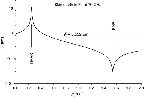
with the effective permeability ![]() . Only the wave with Im(k) > 0 can propagate into metal. The magnetic skin depth δ = 1/Im(k) depends on frequency ω but also on magnetic field H and material parameters Ms, γ, and α. An example of field dependence of δ at the frequency of 70 GHz calculated for an isotropic material with material parameters typical for iron is shown in Figure 15.2. The skin depth shows the typical magnetic field dependence with the maximum at antiresonance (FMAR) and minimum at the resonance (FMR) fields corresponding to the Kittel’s resonance conditions for a planar tangentially magnetized film. As can be seen, the magnetic skin depth changes by nearly three orders of magnitude. Whereas at FMAR the skin depth is more than 20 times larger than the nonmagnetic skin depth δ0, at FMR it is more than 20 times smaller. This indicates that only few tens of nm on the Fe surface are involved in the FMR.
. Only the wave with Im(k) > 0 can propagate into metal. The magnetic skin depth δ = 1/Im(k) depends on frequency ω but also on magnetic field H and material parameters Ms, γ, and α. An example of field dependence of δ at the frequency of 70 GHz calculated for an isotropic material with material parameters typical for iron is shown in Figure 15.2. The skin depth shows the typical magnetic field dependence with the maximum at antiresonance (FMAR) and minimum at the resonance (FMR) fields corresponding to the Kittel’s resonance conditions for a planar tangentially magnetized film. As can be seen, the magnetic skin depth changes by nearly three orders of magnitude. Whereas at FMAR the skin depth is more than 20 times larger than the nonmagnetic skin depth δ0, at FMR it is more than 20 times smaller. This indicates that only few tens of nm on the Fe surface are involved in the FMR.
15.2.2 Exchange-conductivity effects
So far we have neglected the exchange coupling. In a bulk ferromagnetic insulator, where the RF magnetization m is nearly uniform, the exchange interactions play only a minor role. In ferromagnetic metals, however, the RF magnetization is highly nonuniform due to the skin effect, and the exchange effects become important also in bulk samples. To take into account the exchange coupling the term A∇2m/μ0Ms, where A is the exchange stiffness constant, must be introduced into the effective field heff in Eq. (15.2). Using the plane wave solution, as previously, we get the same relations for the components of permeability tensor as those in Eqs. (15.8a) and (15.8b), but the field H must be now replaced by H + Ak2/μ0Ms. Thus the effective permeability μeff depends also on the wave vector k, and Eq. (15.9) represents a bicubic equation for k. The three pairs of roots correspond to three branches of waves propagating in the positive or negative direction of the y-axis. For any particular orientation of static magnetization M0 with respect to the air–metal boundary (plane xz) the secular equation is of the fourth order in k2 with four pairs of roots. In the case of tangentially magnetized half-space, investigated here, the fourth wave branch corresponds to the skin effect in a nonmagnetic metal (μeff = μ0), which takes place if the RF field h is polarized along the static magnetization M0.
Among the four branches of waves propagating in a ferromagnetic metal, we can distinguish two electromagnetic and two of spin-wave branches. In the limit of zero exchange, the electromagnetic branches belong to purely electromagnetic waves investigated in the previous subsection. In a lossless insulator limit, the spin-wave branches correspond to pure spin waves. The interaction between the branches due to electric conductivity results in a mixed electromagnetic and spin-wave character of actual waves (for a detailed discussion, see Patton, 1976). The consequences of this wave hybridization are the exchange conductivity effects, which lead to the shift and broadening of resonance curves due to excitation of spin waves and additional (eddy current) losses. The amplitude of individual waves excited by the RF field can be determined from the boundary conditions at the air–metal interface. If some sample dimensions are smaller than the penetration depth of the ‘Larmor’ spin-wave branch, as for example in thin films, then the standing spin-wave resonances (SWRs) can be observed.
15.2.3 Boundary conditions and surface impedance
In FMR experiments usually the power absorbed by the sample Pabs is measured. According to the Poynting theorem this power is given by
where S in the surface of the sample, n the inward normal of the surface, ht the tangential component of RF magnetic field and η = et/ht the surface impedance. For the metallic half-space with exchange coupling neglected (investigated in Section 15.2.1) the surface impedance η = − ikρ, with k determined from Eq. (15.9), can be easily obtained from the Maxwell equation (15.4). If, however, the exchange coupling is taken into account, all individual wave branches should be included. Their amplitudes can be calculated from the air–metal boundary conditions. The standard electromagnetic boundary conditions, requiring the continuity of tangential components of electric and magnetic fields and the normal component of magnetic induction, must be supplemented by the exchange boundary condition (Rado and Weertman, 1959)
where Esurf is the surface anisotropy energy density. Frequently only the two limit cases: completely free surface spins (∂m/∂n = 0) or fully pined spins (m = 0) are considered.
If the amplitude of tangential component of RF magnetic field ht on the sample surface is constant during FMR experiment, the resonance curve is determined by the field dependence of surface impedance η itself. This condition, however, can be fulfilled only if the sample represents only a little load to the measuring circuit. In more complicated situations and for some applications, the solution of Laplace equation (15.6) is required. Then the surface impedance can be used in the boundary condition for the sample surface. Generally the analytic expression for η is rather complicated. For some purposes the simple solution obtained in the local approximation η = − ikρ is sufficient. Then the resonance field of metallic half-space with static magnetization M0 at any angle to the surface can be obtained from the Kittel’s resonance condition for a thin film magnetized at the same angle.
Concluding this section, we should note that the theory of FMR for the planar air–metal boundary can be used also for bulk metallic samples of any shape if the radius of surface curvature is much larger than the magnetic skin depth. In this case, however, we should keep in mind that the orientation of static magnetization M0 with respect to the sample surface and the corresponding resonance field can vary over the surface. Then the resonance is inhomogeneously broadened and the total resonance curve is obtained as the envelope of local resonance curves.
15.3 Characteristic features of FMR in wires
FMR in metallic wires exhibits some particular features. They are mainly:
• Dependence of surface impedance on wire diameter
• Electric polarization of the wire
As we have already mentioned, FMR in metallic samples substantially differs from FMR in insulators. The basic resonance mode in an insulator sample is the uniform precession mode. The nonuniform resonance modes are observed only if the RF exciting field or the exchange boundary condition are nonuniform. Due to the skin effect, however, metallic samples are more predestined to appearance of nonuniform resonance modes. Particularly, if some dimensions of the sample become comparable to the skin depth, the magnetostatic or dipole-exchange modes can be intensely excited. As we have shown in Section 15.2.1 the magnetic skin depth depends on the applied magnetic field. It is maximum at FMAR and minimum at FMR. The effect of sample dimensions on FMAR therefore appears already for dimensions much larger than the classical skin depth. However, for FMR it becomes most remarkable at submicron dimensions.
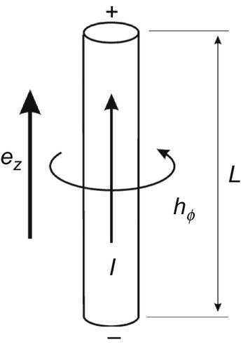
The effect of electric polarization utilizes the large aspect ratio of the wire sample. When a conducting body is placed in an external electric field, the electric charges on its surface rearrange so that the electric field in the interior vanishes. This leads to electric polarization of the body and appearance of electric dipole moment. In the RF electric field the alternating electric charges on the surface produce electric current along the wire and strong circumferential magnetic field hϕ in the wire (see Figure 15.3). The influence of polarization effect on FMR in elongated metallic specimens was first investigated by Rodbell (1959a,b). For a large-aspect ratio the electric charges at the ends can be approximated by point charges ± q ∝ ezL2, where L is the sample length and ez the projection of electric field e into its axis. Then the circumferential RF magnetic field hϕ is proportional to L2 and the absorbed power to L5, as was experimentally verified (Rodbell, 1959b). The circumferential field can be several orders of magnitude larger than the microwave magnetic field in an empty microwave cavity or waveguide. If the wire is placed in free space and its length is equal to an odd multiple of electromagnetic half-wavelength, it can act as a dipole antenna. Then the circumferential field can be even much more enhanced. The polarization effect can substantially increase the sensitivity of FMR measurements. As will be shown in Section 15.7, it can also be used for investigation of nonlinear phenomena in ferromagnetic metals.
There is another feature by which the FMR in a metallic wire differs from FMR in a long insulator cylinder. FMR in an insulating sample does not depend on microwave electric field e in the sample and its surrounding. Therefore, in an isotropic insulator cylinder the resonance field depends only on the angle between the static magnetic field and the sample axis. Two basic orientations can be denoted as: PC—parallel configuration, with the static field along the wire axis, and TC—transversal configuration, with the static field perpendicular to the axis. As a consequence of conductivity the resonance field and the line shape in the metallic wire are also sensitive to the magnitude of microwave electric field e in the wire proximity and its orientation with respect to wire axis. It is therefore useful to extend the nomenclature for some basic experimental configurations (Figure 15.4). The letter e denotes the situation when electric field is parallel to the wire axis. In this case the polarization effect is strong. The letter h is used for electric field perpendicular to the wire axis and the microwave magnetic field parallel to it. For such configuration the electric polarization of wire is absent. The other possible orientations of microwave fields are not considered because they have not been used in the experiments described in the following sections. The configuration PCh correspond to ‘parallel pumping’, which is usually used for investigation of nonlinear effects. It, however, is useless for standard FMR measurements because field h is parallel to static magnetization M0. As will be shown later, using different orientations of microwave fields, different resonance modes can be excited.

15.4 Experimental techniques
FMR is usually measured at microwave frequencies (from a few GHz up to about 100 GHz) and the applied magnetic fields range from 0 up to a few T. In principle the FMR measurement can be done in two different ways. Either the frequency is kept constant and magnetic field changes or at constant field and varying frequency. The old and commonly used method is the FMR spectrometer. Very often the conventional EPR spectrometer is used for this purpose. A simplified block diagram of such spectrometer is shown in Figure 15.5. The microwave power is supplied by klystron or other microwave generator. The power reflected from the device under test (DUT) containing the sample is measured by microwave detector. DUT can be microwave cavity, short-ended waveguide or other microwave device. To increase the signal-to-noise ratio, the field modulation technique is used. The reference signal from lock-in amplifier is amplified and fed to a modulation coil, which modulates the external field with the reference frequency. The signal from the detector is lock-in amplified at this frequency. The output of the lock-in amplifier is then proportional to the field derivative of the reflected power. The high-quality microwave cavities supplied with the commercial spectrometers are designed for the cavity perturbation technique, which is suitable for the measurements of insulating samples with a small magnetic moment. They can be used also for very thin metallic films. Larger metallic samples, however, represent large load to the cavity and can completely smear out its characteristics, particularly if the sample is in the place a where the electric field is nonzero. Therefore, for metallic samples other arrangements are used. Most frequently short-ended waveguides are employed. If a part of sample surface is planar it can be used as a part of the waveguide wall. Then electric field on the surface is nearly zero, and only microwave magnetic field excites the resonance. This method, however, cannot be used for thin wires. A suitable waveguide device for wire samples is shown in Figure 15.6. It consists of a rectangular TE10 waveguide, short-ended by a tuning plunger. The holes for inserting the sample are drilled in the centre of wide sides. It can be used for the measurements in both PCe and TCe configurations. By changing the distance x of the plunger from the sample, the magnitudes of microwave fields e and h at the sample position can be changed. For odd multiples of λg/4, where λg is the wavelength in the waveguide, the magnetic field h is zero, and the electric field e is maximum. At this position the electric polarization of wire is most effective. On the other hand, for even multiples of λg/4 the electric field is zero and magnetic field is maximum. As will be shown later, by changing the plunger position the excitation of various resonance modes can be controlled.


With the development of broadband microwave sources other types of experimental techniques for FMR measurement began to be frequently used. The most commonly used method is the network-analyzer ferromagnetic resonance (NA-FMR). In this case the scattering parameters (S parameters) of a sample fixture are measured as a function of frequency at constant magnetic field. One-port or two-port fixtures can be used. Some fixtures for the measurements of wire samples are shown in Figure 15.7. A one-port coaxial arrangement (Britel et al., 2000) is shown in Figure 15.7a. The wire forms the central conductor of a segment of shorted coaxial line with air as the dielectric. The length of the wire, L, obeys the condition L < λg/4. The second one is a two-port DUT consisting of an interrupted microstrip line with the wire bridging the gap (Kraus et al., 2009). A simple test fixture is shown in Figure 15.7c. The rear side of a SMA connector is flattened by a milling cutter, and the contacts between the sample and the inner and outer conductors are made by silver paint (Raposo et al., 2010). A portion of rectangular TE10 waveguide (similar to that shown in Figure 15.6) was also used for the measurements of transmission parameters (Carbonell et al., 2010). The advantages of NA-FMR are the wide range of measuring frequencies and the possibility to evaluate both the real and imaginary parts of impedance. The disadvantages, however, are the lower sensitivity of measurements and more difficult interpretation of experimental results. As the parameters of the DUT itself also depend on frequency, the evaluation of sample impedance from the scattering parameters is sometimes rather difficult. The network analyzer is suitable for measurements of load impedances around 50 Ω. For impedances much smaller or much larger, the precision of measurements decreases. Then the impedance analyzer is more convenient.

Various modifications of the two methods described earlier were used for FMR measurements in wires. Other possibility, which wire samples offer, is the simultaneous observation of FMR and electric transport properties. For example, low-frequency current passing through microwires can modulate the microwave absorption at resonance (García-Miquel et al., 2012). On the other hand, increase of absorption at resonance raises the wire temperature, which can be measured by means of its electric resistance (Kraus, 2015b). FMR in nanowires can be detected also by DC voltage appearing between its ends due to the rectifying effect. The precession of magnetic moment causes oscillations of resistance originating from the anisotropic magnetoresistance. These oscillations combined with RF current generate the dc voltage (Yamaguchi et al., 2007).
15.5 Parallel field configuration
15.5.1 Theoretical model
From the theoretical point of view the parallel configuration (PC) is much simpler for investigation because for the static magnetic field parallel to the wire axis the problem is axially symmetric. Absorption of microwaves by a long metallic cylinder magnetized to saturation along its axis was investigated by several authors using different approaches (Kraus, 1982; Lofland et al., 2002; Arias and Mills, 2001); for details, see Kraus et al. (2011).
The theory of FMR in an axially magnetized metallic cylinder is similar to that described in Section 15.2 for metallic half-space. The solution, however, is assumed in the form of cylindrical waves
where r, ϕ, and z are the cylindrical coordinates, n is an integer number, Jn(x) the Bessel function and k and β represent the propagation constants in radial and axial directions, respectively. For wire diameter much smaller than the electromagnetic wavelength the dependence on the coordinate z can be neglected and β put zero. Substituting solution (15.12) with β = 0 into the linearized equations (15.2) and (15.5), we get the dispersion relation (15.9) for the radial propagation constant k. It should be noted that it is independent of azimuthal mode number n and is the same as for the metallic half-space. Thus the discussion of Sections 15.2.2 and 15.2.3 applies also to metallic wires.
If the exchange effects are neglected μeff is independent of k, and Eq. (15.9) has only one solution. Then the circumferential components of magnetic field hϕ and the axial electric field ez for the azimuthal mode number n are (Kraus et al., 2011).


and the corresponding surface impedance ηn is given by

where a is the wire radius. As can be seen, besides the material parameters, frequency and magnetic field, the surface impedance depends also on wire diameter and the mode number n. General solution of Eqs. (15.2) and (15.5) is given by a linear combination of particular solutions (15.13) and the total absorption of the wire by the sum of absorptions Pn by individual resonance modes, where
The intensity of a particular mode depends on the actual microwave field h in the wire and on its coupling to the RF magnetization m(n) of the given mode, which is proportional to ![]() . It is evident that homogeneous field h couples only with the resonance modes with odd mode numbers n, whereas the circumferential field produced by electric polarization of wire couples only with the modes of even n. The RF magnetization m(n) of the first two and most important modes (n = 0 and 1) are schematically shown in Figure 15.8. The n = 0 mode is cylindrically symmetric with the closed flux vortex-like structure. It is called the circumferential mode because it couples strongly with the circumferential magnetic field. In most experimental arrangements this is the most intensive resonance mode. From Eq. (15.14) we get the surface impedance
. It is evident that homogeneous field h couples only with the resonance modes with odd mode numbers n, whereas the circumferential field produced by electric polarization of wire couples only with the modes of even n. The RF magnetization m(n) of the first two and most important modes (n = 0 and 1) are schematically shown in Figure 15.8. The n = 0 mode is cylindrically symmetric with the closed flux vortex-like structure. It is called the circumferential mode because it couples strongly with the circumferential magnetic field. In most experimental arrangements this is the most intensive resonance mode. From Eq. (15.14) we get the surface impedance

which is the well-known formula for GMI in wires (Knobel et al., 2003). The mode n = 1 resembles the uniform precession mode of an insulating cylinder. The magnetic charges appearing inside and on the surface of the cylinder produce a dipole-like magnetic field. It is therefore called the dipolar mode. This resonance mode strongly couples with the uniform microwave magnetic field and can be observed only if the circumferential mode is suppressed.

The resonance curve of the mode with number n is determined by the dependence of power absorption Pn on applied magnetic field or on microwave frequency, depending on the used experimental method. Equation (15.15) is suitable only for the cavity perturbation technique, where the sample represents only a small load of the measuring circuit and the field hϕ(n) on the sample surface can be assumed to be constant during the measurement. To get the accurate resonance curve the field (or frequency) dependence of hϕ(n) must be known. In principle, it could be obtained from the solution of the Laplace equation for the actual sample fixture with the electromagnetic boundary conditions at the fixture walls and the sample surface. Because this is practically an insoluble problem, some approximation must be used. Lofland et al. assumed the incident electromagnetic wave in the form of a planar wave, which is suitable for rectangular waveguides or microwave cavities (Lofland et al., 2002). Kraus, on the other hand, proposed to expand the incident radiation into cylindrical waves (Kraus, 1982). The ratio of absorbed-to-incident power Pn/Pin is then given by ![]() , where An is the corresponding scattering moment. The expressions for the scattering moments of both the planar and cylindrical waves can be found in Kraus et al. (2011).
, where An is the corresponding scattering moment. The expressions for the scattering moments of both the planar and cylindrical waves can be found in Kraus et al. (2011).
It is interesting to observe how the resonance modes n = 0 and n = 1 change when the wire diameter decreases from micrometric to nanometric dimensions. For wire diameters much larger than the skin depth the RF magnetization is confined to a thin layer under the surface as schematically shown in Figure 15.9. For n = 0 the layer is magnetized in the circumferential direction. This is equivalent to the case of tangentially magnetized metallic half-space for which the Kittel’s resonance condition of a tangentially magnetized thin film

can be used, as discussed in Section 15.2. For the mode n = 1 the situation is similar, with the exception that the layers in the upper and lower parts are magnetized in the opposite sense, and small magnetic charges appear where these two parts head each other. The resonance condition (15.17) holds in this case as well. The situation changes when the ratio δ0/a increases. The most significant changes are observed when the wire radius is comparable to the nonmagnetic skin depth δ0. The absorption curves of the two resonance modes, calculated for Fe wires of different diameters at the frequency of 70 GHz, are compared in Figure 15.10. For δ0/a ~ 1 the resonance curves become broad and distorted. With further decrease of diameter the curves again narrow. For the circumferential mode (n = 0), the resonance field remains unchanged but the absorption peak overturns to an absorption dip. For the dipolar mode the (n = 1) the resonance field shifts to lower values. It is caused by an increase of dipolar energy because the volume and surface magnetic charges increase.


For wire diameters much smaller than the skin depth, the RF magnetic field penetrates into the whole volume (see the lower row in Figure 15.9). The dipolar mode now becomes equivalent to the uniform precession of magnetization in an insulating cylinder, and the resonance field satisfies the Kittel’s resonance condition
The resonance fields calculated from Eqs. (15.17) and (15.18) are denoted by the vertical dotted lines in Figure 15.10.
When the exchange coupling is taken into account the theory becomes more complicated. As was mentioned in Section 15.2, in this case the secular equation (15.9) becomes bicubic, and three wave branches (one electromagnetic and two spin-wave) must be taken into account. The analytical expression for the surface impedances ηn was derived in Kraus et al. (2011) for three different types of surface magnetic anisotropy. Using the surface impedance ηn in the expressions for the scattering moment An, shown in the same reference, the resonance curves can be calculated. Numerical simulations for wires made of different materials verified the presence of the same exchange effects as those already known from planar samples, such as:
• Exchange-conductivity broadening of resonance curve (Ament and Rado, 1955)
• Existence of surface spin-wave modes for some kinds of surface anisotropy (Murtinová and Frait, 1972)
• Radial standing SWRs in very thin wires
Another effect, which does not have analogous counterpart in thin films, was discovered. It is the exchange shift of the main resonance field of the circumferential mode in very thin wires. Because the exchange energy for the vortex-like structure (Figure 15.8) increases with decreasing wire diameter, the resonance field shifts downward. The numerical calculations proved that the shift is proportional to 2A/(μ0Msa2) (Kraus et al., 2011).
15.5.2 Experimental results
FMR measurements on single amorphous wires have been described in many papers. For the measurements both the conventional FMR and NA-FMR techniques have been used. The wire diameters were few μm and more, for which the condition δ0/a ![]() 1 is well satisfied. Moreover, usually no care was taken of the electric polarization of the wire. Therefore, mainly the circumferential mode was excited, and for the interpretation of such experiments the resonance condition (15.17) should be used. Possible magnetic anisotropy was included by adding the anisotropy field HK to H0. The influence of decreasing wire diameter on FMR in individual wires has been systematically investigated only by Lofland et al. (2002) and by Kraus and Jirsa (1984) and Kraus et al. (2011, 2012, 2013).
1 is well satisfied. Moreover, usually no care was taken of the electric polarization of the wire. Therefore, mainly the circumferential mode was excited, and for the interpretation of such experiments the resonance condition (15.17) should be used. Possible magnetic anisotropy was included by adding the anisotropy field HK to H0. The influence of decreasing wire diameter on FMR in individual wires has been systematically investigated only by Lofland et al. (2002) and by Kraus and Jirsa (1984) and Kraus et al. (2011, 2012, 2013).
Lofland et al. investigated wires with diameters from 3 to 6 μm in the frequency range 10–60 GHz. The conventional cavity perturbation technique was used. The sample was carefully located in the cavity such that the RF electric field at the wire was close to zero. The absorption curves were rather distorted, but the characteristic resonances were observed at the fields satisfying the resonance conditions (15.17) and (15.18). Whereas at the lower resonance field the peak of absorption was observed, at the higher one a dip in absorption (reminiscent of FMAR) appeared. From what was shown before, it seems evident that the two resonance modes n = 0 and 1 were observed in this experiment. The lower resonance corresponded to the dipolar resonance mode, whereas the upper one corresponded to the weak circumferential mode (due to the residual electric field at the sample). Also the dip of absorption for very thin wires has been theoretically predicted.
The FMR measurements on a glass-coated amorphous wire Fe76Si9B10P5 with the diameter 2a = 1.5 μm (Kraus et al., 2011), and a series of wires Fe77.5Si7.5B15 with diameters ranging from 133 nm to 25 μm (Kraus et al., 2012) confirmed the existence of the two resonance modes. For the measurements, the PCe configuration and a short-ended waveguide were used. The exception from the sample fixture shown in Figure 15.7 was that a circular waveguide was employed. By changing the position of the tuning plunger, the intensity of electric field at the sample position could be changed. Examples of resonance curves, measured with maximum electric field at the sample, for two wires with different diameters are shown in Figure 15.11. These resonance curves correspond to the circumferential resonance modes (n = 0) excited by electric polarization of the wire. The resonance curve of the thick wire (2a = 25 μm) shows a broad antiresonance (FMAR) dip at lower field and narrow resonance (FMR) peak at higher field. As expected, both the antiresonance and resonance fields well satisfy the Kittel’s resonance conditions for a tangentially magnetized planar film (the dotted lines). When the wire diameter decreases, the resonance curves start to change. First, the antiresonance broadens and finally disappears for diameters less than about 10 μm. This can be well understood because at FMAR the magnetic skin depth becomes much larger than the wire radius (see Figure 15.2), and the antiresonance is smeared out. With decreasing diameter the intensity of resonance peak decreases and its position and shape little change. The small shift to lower fields is caused by an increase of axial anisotropy due to larger tensile stress produced by the glass coat. The splitting of the main resonance may be ascribed to the surface spin wave. The resonance peak of surface mode appears above the main (bulk) resonance peak. It was found that with decreasing wire diameter the relative intensity of the surface mode increases at the expense of bulk resonance, as can be expected. The experimental curve can be well fitted with the perpendicular surface anisotropy Ks ≈ 6 10− 4 J/m2 (see the dotted curve). It has been theoretically predicted (Kraus, 1982) and experimentally verified (Kraus and Jirsa, 1984) that in very thin wires radial standing spin waves can be excited. On the magnified part of low-field side of resonance curve shown in Figure 15.11 a tiny ripple can be seen. The period of the ripple increases with increasing distance from the main resonance field and scales as 1/a2 for wires with different diameters. From the theoretical fit of the experimental curve the exchange stiffness constant A = 8.2 10− 12 J/m was obtained.
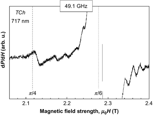
When the tuning plunger is moved to the distance x close to an integer multiple of λg/2, the electric field at the sample position is substantially reduced, and the intensity of circumferential resonance mode decreases nearly by three orders of magnitude. Then on very thin wires the dipolar resonance mode (n = 1) can be observed. The resonance curve measured on the wire with the diameter of 717 nm is shown in Figure 15.12. The peak at lower fields corresponds to the dipolar mode (n = 1). The resonance field calculated from the Kittel’s resonance condition (15.18) is shown by the dotted line. The peak observed at higher field corresponds to the residual circumferential resonance mode (n = 0) because the microwave electric field is not exactly zero. The theoretically calculated resonance curve for the dipolar mode is also shown in the figure. For wires with diameters larger than 10 μm, the dipolar mode could not be observed, in agreement with the theoretical prediction.

 . The vertical dotted lines correspond to resonance fields calculated from Kittel’s resonance conditions. Reprinted with permission from Kraus et al. (2012). © 2012 American Institute of Physics.
15.6 Transversal field configuration
Transversal field configuration (i.e., static magnetic field perpendicular to the axis) is the second most commonly used configuration for FMR measurements in cylindrical samples of ferromagnetic insulators. For bulk metallic samples this configuration is less appropriate because the skin effect leads to the inhomogeneous broadening of resonance curve, as was mentioned in Section 15.2. Both configurations PC and TC are, however, frequently used for the investigation of magnetic anisotropy in arrays of self-organized magnetic nanowires. It is therefore useful to know how the FMR spectra depend on wire diameter.
Theoretical description of FMR in transversal configuration is much more difficult because the cylindrical symmetry is broken. Therefore only approximate models for two limit cases of large and small wire diameter will be discussed. Two polarization arrangements TCe and TCh (see Figure 15.4) will be investigated.
15.6.1 Theoretical models
For thick wires, where the skin depth is much smaller than the wire diameter, the strong-skin-effect approximation (SE) is used (Kraus et al., 2012). Then the dynamic components of the fields are confined to a very thin layer on the wire surface (Figure 15.13). Neglecting the exchange-conductivity effect, the dynamics of the skin layer can be approximated by uniform precession of magnetization. Then the local resonance field can be calculated from the Kittel’s resonance condition of an obliquely magnetized thin film

where ϕ is the angle between the DC field and the local normal ur of the surface. It should be noted that the demagnetizing field − Ms/2 of transversally magnetized long cylinder has been taken into account. The resonance field varies between the minimum value for ϕ = π/2 and the maximum one for ϕ = 0. The resulting absorption curve is given by the envelope of the local resonance curves (Gurevich and Melkov, 1996)

whereμ0 is the permeability of free space, ![]() and
and ![]() the imaginary parts of diagonal elements of susceptibility tensor, and hx, hy the components of RF field perpendicular to the DC field. For TCe configuration we have hx = 0,
the imaginary parts of diagonal elements of susceptibility tensor, and hx, hy the components of RF field perpendicular to the DC field. For TCe configuration we have hx = 0, ![]() cos ϕ and for TCh configuration hx = h, hy = 0. The absorption curves calculated using the material parameters of amorphous Fe77.5Si7.5B15 alloy are shown in Figure 15.14. For TCh configuration there are two well-distinguished maxima on the curve near the resonance fields corresponding to ϕ = 0 and ϕ = π/2. For TCe configuration the lower maximum is suppressed because the part of surface close to ϕ = π/2, where the circumferential magnetic field is parallel to the static field, does not contribute to the resonance.
cos ϕ and for TCh configuration hx = h, hy = 0. The absorption curves calculated using the material parameters of amorphous Fe77.5Si7.5B15 alloy are shown in Figure 15.14. For TCh configuration there are two well-distinguished maxima on the curve near the resonance fields corresponding to ϕ = 0 and ϕ = π/2. For TCe configuration the lower maximum is suppressed because the part of surface close to ϕ = π/2, where the circumferential magnetic field is parallel to the static field, does not contribute to the resonance.


When the skin depth is much larger than the wire diameter, the electromagnetic field fully penetrates into the sample volume, and the quasi-static (QS) approximation can be used (Boucher and Ménard, 2010). For TCh configuration the situation is quite simple. The microwave field h and consequently the dynamic magnetization m can be assumed to be uniform over the sample volume. Then the Kittel’s resonance condition for the transversally magnetized long cylinder

can be applied.
For TCe configuration the situation is much more complicated. In QS approximation the RF current I induced by electric polarization of the wire can be considered to be uniform. Then the RF circumferential field hϕ = 2Ir/(πd2) is proportional to the distance r from the wire axis. The inhomogeneous field hϕ can excite spatially nonuniform oscillations of magnetization, such as magnetostatic or dipole-exchange modes. Though the magnetostatic modes of an axially magnetized cylinder had been known for a long time (Joseph and Schlömann, 1961), the continuum theory for transversally magnetized cylinder was missing until recently. The microscopic model of dipole-exchange modes (Nguyen and Cottam, 2005) could hardly be used because it requires complicated numerical calculations. Magnetostatic waves are relatively long-wavelength oscillation for which the exchange interactions can be neglected. They can be obtained by solving the Walker magnetostatic equation with appropriate electromagnetic boundary conditions (Walker, 1957). In an infinite isotropic medium they are plane waves satisfying the dispersion relation (Gurevich and Melkov, 1996)

where ϕ is the angle between the wave vector k and the direction of static magnetization M0. If the demagnetizing field of a transversally magnetized infinite cylinder is included into H0 one gets Eq. (15.19). Because any bulk magnetostatic mode can be expanded into a series of plane waves the energy of bulk magnetostatic modes of transversally magnetized cylinder must lie in the energy band determined by Eq. (15.19). An approximate solution of Walker equation for transversally magnetized long cylinder is reported in Kraus et al. (2013). We have found that solutions that satisfy the boundary condition and couple with the circumferential field hϕ can be obtained when the diagonal element μ of the Polder permeability tensor satisfies the approximate relation
which implies the resonance conditions
This equation gives the resonance frequencies of two magnetostatic modes. It can be alternatively described by Eq. (15.19) with ![]() and
and ![]() . As will be shown later, the two magnetostatic modes can be excited in submicron wires using TCe configuration.
. As will be shown later, the two magnetostatic modes can be excited in submicron wires using TCe configuration.
So far we have investigated the limit cases of very thick and very thin wires. At present there is no theory for an intermediate case when the wire diameter is comparable with the skin depth.
15.6.2 Experimental results
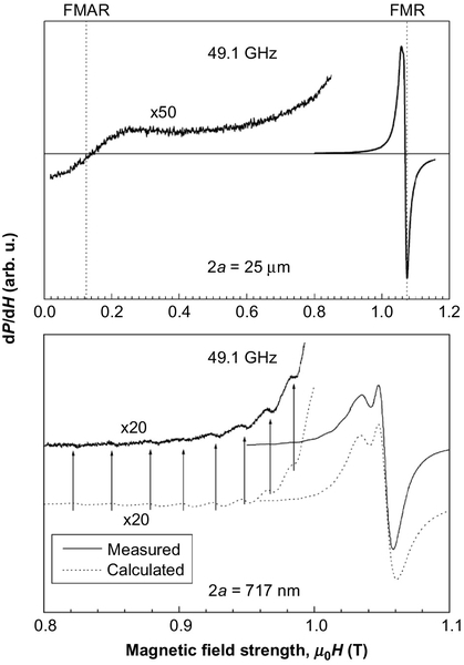
In TCe configuration a strong FMR signal is obtained due to electric polarization of the wire. As the RF magnetic field h in the waveguide is parallel to the DC field H0 (see Figure 15.4), it does not contribute to FMR. Thus in this configuration only the resonance modes excited by the circumferential magnetic field hϕ are observed, and their intensity is proportional to e2. The resonance curves measured at frequency of 49.1 GHz on amorphous wires Fe77.5Si7.5B15 with different diameters are shown in Figure 15.15. Similar spectra were observed also at 69.7 GHz (Kraus et al., 2013). For the thick wires two resonances can be distinguished, the strong one at the higher field and the weak one at the lower field. For the 25-μm wire they are closest to the limits (ϕ = 0 and π/2) of the inhomogeneously broadened resonance curve calculated in the SE approximation (Figure 15.14). The lower peak is much weaker, which is in agreement with the theoretically calculated curve in TCe configuration. With decreasing wire diameter the peaks broaden and shift closer to the centre. Finally, for submicron wires two very narrow resonances are observed with resonance fields corresponding to the magnetostatic modes (ϕ = π/6 and π/3).

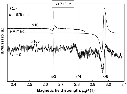
If the electric field e in the TCh configuration was exactly perpendicular to the wire axis, only the nearly uniform h would contribute to FMR. This is, however, hardly achieved, particularly in the cylindrical waveguide. There is therefore always a small component of electric field parallel to wire axis producing the circumferential magnetic field hϕ. Even if the electric field is weak, the circumferential field may be rather high. To be able to observe the resonance excited by the uniform field h the plunger must be finely tuned to get the minimum electric field at the sample. This is illustrated in Figure 15.16, where the resonance curves measured at two different positions of the tuning plunger are shown. While at the position where e is maximal both magnetostatic modes can be observed, at e = 0 only the upper one can be seen, and the weak uniform precession mode appears at ϕ = π/4. The dependence of FMR spectra on wire diameter, measured at 49.1 GHz with minimum electric field at the sample position is shown in Figure 15.17. For the wires with diameters d = 25, 14, and 9.6 μm two resonance peaks can be distinguished. The positions of both peaks well correspond to those observed in the TCe configuration (Figure 15.15). In this case, however, the intensities of both peaks are comparable as predicted theoretically for TCh configuration. The splitting of the lower peak for wire diameter 25 μm can be ascribed to the surface spin wave as in the case of PCe configuration. For the wire diameters close to the nonmagnetic skin depth, the peaks are very broad and the FMR signal is hardly distinguishable. For submicron wires again two narrow peaks appear but at new positions. The upper one (ϕ = π/6) is the residual magnetostatic mode, and the lower one (ϕ = π/4) corresponds to the uniform precession mode. For wires with diameters 318 and 133 nm, the FMR signal is already hidden in the noise.

Similarly as in the parallel configuration in the transversal configuration the standing spin waves can also be excited in submicron wires. The magnified resonance curve measured in TCh configuration with maximum electric field at the sample is shown in Figure 15.18. In this case both the uniform precession mode (ϕ = π/4) and the upper magnetostatic mode (ϕ = π/6) can be excited. The tiny ripple can be attributed to the standing dipole-exchange modes. In contrast to the parallel field configuration, where the spin-wave peaks appear only on the low-field side of the main resonance, in the normal configuration the spin-wave peaks can be found on both sides of the upper magnetostatic resonance mode. The theory of dipole-exchange modes in transversally magnetized cylinders is, unfortunately, missing.
In summary of this session we can say that the resonance peaks observed in transversally magnetized wires can be described by the general resonance condition (15.19) with several discrete values of the angle ϕ. The angles 0 and π/2 correspond to the upper and lower limits of inhomogeneously broadened resonance peak in thick wires. The angles π/6 and π/3 give the resonance fields of the upper and lower magnetostatic modes excited by the circumferential RF field. And finally, the angle π/4 belongs to the uniform precession mode of very thin wires, which is excited in nearly uniform RF field.
15.7 Nonlinear FMR in thin wires
Applications of magnetic microwires and nanowires in microwave and spintronic devices may involve large RF currents flowing through the wires. They may result in a large precession of magnetization and related nonlinear effects, such as frequency multiplication, additional power losses, soliton wave propagation, and others. The nonlinear effects, therefore, can play a crucial role in practical applications. Nonlinear FMR is an ordinary experimental technique for investigation of nonlinear effects in spin dynamics. Until recently, most experimental work on nonlinear FMR involved only yttrium iron garnet (YIG) and similar materials because they possess small Gilbert damping and require lower RF fields to induce the nonlinear behaviour (for a review of early works, see, e.g., Patton, 1984). In metals, where the resonance linewidth is of the order of 10− 2 T, large microwave powers (up to few kW) were required to achieve the threshold fields for the onset of spin-wave instabilities (Bertaud and Pascard, 1966). Therefore only a few high-power FMR investigations of Permalloy thin films have been published until recently (An et al., 2004). There has been a resurgence of interest in nonlinear effects in ferromagnetic metals because of increasing applications of such materials in magnetic recording. New experimental techniques have been developed, which allow to investigate the nonlinear phenomena in metallic thin films using moderate and low-power microwave generators (Gertis et al., 2007; Khivintsev et al., 2011).
As already mentioned in Section 15.3, polarization effect in metallic wires can substantially enhance the circumferential RF field in the sample. This allows to achieve the large critical fields for the onset of nonlinear effects in ferromagnetic metals with much lower microwave power than in the conventional high-power FMR experiments. Utilizing this method the butterfly curves for subsidiary absorption (Kraus et al., 1983) and the fine structure of FMR curves under coincidence condition of the main and subsidiary resonances (Kraus, 1983) were observed in glass-coated amorphous microwires.
15.7.1 Suhl spin-wave instabilities
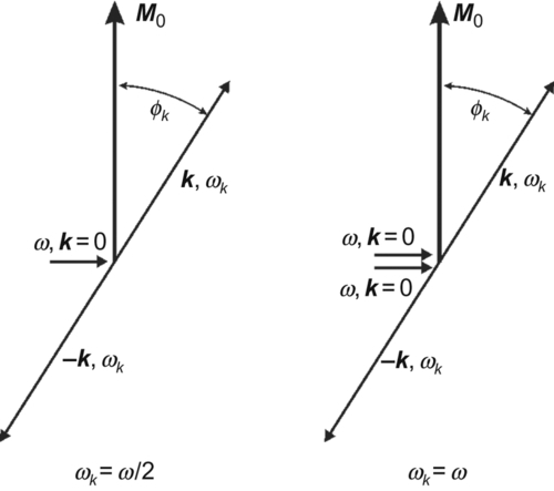
Among many nonlinear effects the most frequently investigated are the saturation of main resonance and the subsidiary absorption at lower applied magnetic fields. These are the first effects that appear when the microwave power is increased above some critical value. The theory of nonlinear FMR in bulk ferromagnetic insulators was developed by Suhl (1957). According to the theory these effects arise from the transfer of energy from the uniform precession motion to spin waves. At low signal levels such energy transfer causes only a small additional damping of uniform precession. Above a certain threshold level, however, the uniform precession becomes unstable, and a spontaneous transfer of energy (parametric excitation of spin waves) appears. Two different mechanisms responsible for the subsidiary absorption and the saturation of main resonance are schematically shown in Figure 15.19. In the first-order spin-wave instability one magnon with k = 0 (uniform precession) splits into a pair of magnons with opposite k vectors. This mechanism is responsible for the subsidiary absorption. The second-order spin-wave instability causes the saturation of main resonance. Here two magnons with k = 0 scatter and produce a pair of magnons with k and − k. From the energy conservation rule it follows ωk = ω/2 and ωk = ω for the first-order and the second-order spin-wave instabilities, respectively, where ω is the frequency of uniform precession and ωk the spin-wave frequency, which is given by the dispersion relation

where ϕk is the angle between k and static magnetization M0. The critical field hcrit for the onset of parametric excitation of spin-wave pair (k, − k) is given by

for the first-order instability and by

for the second-order instability, where ΔHk is the spin-wave linewidth and Wk(n) the dimensionless coupling coefficient for nth-order instability. The threshold fields hc are then given by minimization of right-hand sides of Eqs. (15.26) and (15.27) over all available spin-wave states. The spin waves corresponding to the minimum condition are called the critical modes. The coupling coefficients Wk depend on the sample shape, static magnetic field and its orientation and also on the polarization of RF magnetic field h (Patton, 1969). The first-order instability threshold field is usually lower than the second-order one. The dependence of hc on applied DC magnetic field is called the ‘butterfly curve’. The first-order instabilities, however, are not allowed for all magnetic fields. The maximum field, which is restricted by the condition ωk,min = γH0, < ω/2, is called the cutoff field Hc. Above the cutoff field the second-order process comes into play. Far from FMR the coupling coefficient Wk(1) is of order of unity, but at resonance it sharply increases. So if the condition ωres = ω = 2ωk is fulfilled, an exceptionally small threshold field hc of the order ΔH0ΔHk/Ms is observed. This situation is called the coincidence of the subsidiary and the main resonances.
The Suhl theory was developed for bulk isotropic insulators. It can be extended also to finite specimens of small dimensions. Then the spin-wave continuum described by the dispersion relation (15.25) must be replaced by the discrete spectrum the dipole-exchange modes, which leads, for example, to a fine structure of perpendicular or parallel pump instabilities in single crystal YIG spheres (Patton, 1984). The confinement of spin waves in samples with nanometric dimensions substantially reduces the number of spin-wave modes, which are available for parametric excitation (An et al., 2004). For ferromagnetic metals the situation is even more complicated. Due to the skin effect the main resonance mode is not a uniform precession, as assumed in the Suhl’s theory. The modified Suhl model can be applied to very thin films, where the skin effect is negligible (An et al., 2004; Olson et al., 2007). It should be, however, used with a care for thin wires. In analogy to the linear resonance, one can expect that in the case of strong skin effect (δ ![]() a) the thin film approximation can be used also for nonlinear FMR. But for medium and very thin wires, the Suhl’s theory should be substantially changed.
a) the thin film approximation can be used also for nonlinear FMR. But for medium and very thin wires, the Suhl’s theory should be substantially changed.
15.7.2 Subsidiary absorption in amorphous microwires
The conventional high-power FMR technique was used to investigate nonlinear phenomena in glass-coated amorphous FeNiPB and FeCoPB microwires at the frequency of 36 GHz (Kraus and Anisimov, 1986). The sample was placed at the centre of a rectangular TE103 cavity with RF electric field parallel to the wire. Pulse magnetron with a maximum output power of 360 W was used for the measurements. The absorption curves obtained for different levels of incident power are shown in Figure 15.20. The curve for incident power of 0.36 W corresponds to the linear FMR. With increasing incident power the main resonance peak broadens and shifts to higher fields. The shift is caused by the decrease of saturation magnetization due to heating of the sample. At lower fields a broad peak of subsidiary absorption, with the cutoff field Hc about 6 kOe, is observed. As can be seen, by using the electric polarization of wire the microwave power required for achievement of nonlinear effects in ferromagnetic metals can be substantially reduced.

The first butterfly curve for perpendicular pumping, measured on a ferromagnetic metal, was published in 1983 (Kraus et al., 1983). For the interpretation of experimental results the formula for the threshold field hc of a tangentially magnetized thin film, excited by linearly polarized RF field (Patton, 1969), was used. The experimental curve could be well fitted with ΔHk independent of k and ϕk. Unfortunately, the absolute value of ΔHk could not be determined because by that time we were not able to assign the right value of the circumferential field hϕ to the incident microwave power. Later on the problem was roughly solved. The RF electric field on the sample was calculated from the incident power, using quality factor and the reflection coefficient of the cavity (Kraus and Anisimov, 1986). Then the circumferential field on the wire surface was estimated using the antenna theory and some simplifying assumptions. The butterfly curve for an amorphous FeCoPB microwire, obtained in this way, is shown in Figure 15.21. The theoretical curve calculated for a tangentially magnetized thin film with the constant value ΔHk = 96 Oe is shown by the full line. For the fields less than 3.5 kOe, where k ≠ 0, the experimental data quite well follow the theoretical curve. The difference between the theoretical and experimental data in the range 3.5 kOe < H < Hc, indicates that for ![]() ΔHk depends on the direction of spin-wave propagation. The linewidth ΔH0 determined from the butterfly curve is about 65% larger than the linewidth ΔH = 58 Oe of the linear FMR. This may be attributed to an overestimated circumferential field hϕ by the simplified calibration procedure. The cutoff field Hc and the resonance field Hres shown in Figure 15.21 well agree with the values determined from the linear FMR. This proves that the thin film approximation can well explain the subsidiary absorption in thick wires.
ΔHk depends on the direction of spin-wave propagation. The linewidth ΔH0 determined from the butterfly curve is about 65% larger than the linewidth ΔH = 58 Oe of the linear FMR. This may be attributed to an overestimated circumferential field hϕ by the simplified calibration procedure. The cutoff field Hc and the resonance field Hres shown in Figure 15.21 well agree with the values determined from the linear FMR. This proves that the thin film approximation can well explain the subsidiary absorption in thick wires.

15.7.3 Fine structure of nonlinear FMR curves in very thin wires
As mentioned in Section 15.7.1, when the subsidiary and the main resonances coincide, exceptionally low threshold field hc can be obtained. In combination with the electric polarization effect this allows to observe the nonlinear FMR even with conventional FMR equipment. For the resonance frequency given by Eq. (15.17) the coincidence condition ωres = ω = 2ωk requires

which, for example for μ0Ms = 1 T is fulfilled for frequencies less than about 20 GHz.
X-band FMR measurements were performed on glass-coated amorphous microwires of different compositions and diameters. When the incident microwave power exceeded the threshold value a distortion of central part of resonance curve appeared. With increasing power the distortion extended in both directions, and in wires thinner than about 10 μm a fine structure of nearly equidistant sharp peaks could be seen on the distorted part of the curve (see Figure 15.22). It was found that the period δH of fine structure was inversely proportional to the wire diameter (Figure 15.23). For the submicron wires the period δH is so large that only one or two peaks could be observed on the resonance curve. With further increase on incident power other irregular peaks appeared, and the resonance curve became very complex. The development of FMR spectra with increasing incident power for an amorphous submicron wire is shown in Figure 15.24. In the upper part of the figure the measured resonance curves are shown. The corresponding absorption curves, obtained by their numeric integration, are depicted in the lower part. The sharp dip on the absorption curves indicates that at H = 355 Oe the premature saturation of absorption occurs.


The fine structure of nonlinear FMR was explained by the parametric excitation of dipole-exchange modes by the first-order instability process (Kraus and Jirsa, 1984). The dipole-exchange modes of an axially magnetized insulating cylinder were investigated by Lai et al. (1977) and by Arias and Mills (2001). The magnetostatic potential ψ was assumed in the form of cylindrical waves (Eq. 15.12). Unfortunately, no analytical expression for the dispersion relation was given. We have shown that the dispersion relation for the bulk dipole-exchange modes can be expressed by Eq. (15.25) with

(Kraus and Jirsa, 1984), where xm,n are numeric constants. The integer numbers m and n are the radial and azimuthal mode numbers of the given mode. The dependence of characteristic frequency ωm,n on the longitudinal propagation constant β is schematically shown in Figure 15.25. The dependence has a broad minimum at β = βm,n. To get the numbers xm,n the boundary condition problem must be solved numerically. To simplify the solution, the actual boundary conditions are replaced by a simple artificial one ψ(a) = 0, which means Jn(xm,n) = 0. The actual xm,n are then expected to lie between the mth and (m + 1)th root of Bessel function Jn.

The fine structure of the nonlinear resonance can be explained in the following way. Let the RF magnetic field hϕ be kept constant at some value above the minimum threshold field. When the DC magnetic field increases, the energy of the dipole-exchange modes also increases, and the (m,n) branch gradually emerges from the level ω/2. At the moment when the minimum frequency is just equal to ω/2 (as indicated by dotted curve in the figure) the number of states available for parametric pumping sharply increases, and the absorption of sample decreases. The corresponding DC field Hm,n can be calculated from this condition. It should be noted that among the dipole-exchange branches only those with the critical fields lower than the driving field hϕ are effective. The critical field of the particular mode depends on its coupling with the main resonance mode. For example, the modes with odd azimuthal number n cannot be excited at all because they do not couple with the circumferential resonance mode. The experimentally observed periods of fine structure well agree with δH = H1,n − H1,n− 2 for even azimuthal number n, calculated with the exchange stiffness constant A determined from the radial SWRs on submicron wires (Kraus, 2015a). The dipole-exchange modes with radial mode number m = 1 are localized near the surface and well couple with the circumferential resonance mode (n = 0). The increasing complexity of the nonlinear spectrum with increasing power level may be explained by the parametric excitation of the dipole-exchange modes with higher radial numbers m.
Fine structure has been also found on NA-FMR resonance curves measured on an 8.5-μm-thick amorphous microwire Co67Fe4Cr7Si8B14 (Kraus et al., 2009). A periodic ripple was observed above some critical incident power. This behaviour was attributed to the parametric excitation of dipole-exchange modes as described earlier. Later experiments with microwires of different diameters, however, showed that the period of the ripple is independent of wire diameter, but it changes with the length of the cable connecting the sample fixture and the network analyzer. Thus the interpretation of the experimental results was not correct. Possible explanation of this ripple may be the generation of harmonic signals, due to the nonlinear response of the sample, and their interference in the connecting cables. Because the calibration procedure of network analyzers does not take into account higher harmonics of the probe signal, it may lead to a spurious evaluation of S parameters.
15.8 Summary
Due to electric conductivity the FMR in metallic wires exhibits some peculiarities. They are mainly: the highly nonuniform resonance modes due to electric polarization of the wire and the skin effect. The behaviour of FMR depends on the ratio of magnetic skin depth to wire diameter. In the parallel field configuration two resonance modes can be observed—the more intense circumferential mode and a weak dipolar mode. When the wire diameter decreases the two modes behave in different ways.
For the circumferential mode first the antiresonance disappears. This happens when the diameter is less than the antiresonance skin depth, which is usually of the order of 10 μm. For wire diameters less than about 1 μm radial standing spin waves can be observed on the low-field side of the resonance curve. For even thinner wires (few 10 nm) an exchange shift of the circumferential resonance field is expected.
The weak dipolar resonance mode can be observed only if the microwave electric field at the wire is reduced to minimum. For large wire diameters its resonance field coincides with the resonance field of the circumferential mode. When the wire diameter decreases below the nonmagnetic skin depth (about few μm) the resonance field gradually shifts to a new position, which corresponds to the uniform precession mode of an infinite cylinder.
In the case of transversally magnetized wire three different resonance modes can be excited. Due to the skin effect an inhomogeneously broadened resonance peak with two distinct singularities at the edges is observed in thick wires. With decreasing wire diameter the broadening decreases and the resonance spectrum changes. In submicron wires generally three sharp resonance peaks can be observed. The relative intensity of the peaks depends on the particular experimental arrangement. Two magnetostatic modes can be excited by the circumferential RF magnetic field due to electric polarization of the wire. If the RF electric field at the wire is negligible the uniform precession resonance mode appears.
Due to the electric polarization of wires the nonlinear FMR phenomena can be observed at relatively low microwave powers. The subsidiary absorption and premature saturation of the main resonance in thick wires can be well explained by a modified Suhl’s theory of spin-wave instabilities. The fine structure of nonlinear FMR spectra observed in micron and submicron wires was attributed to the parametric excitation of dipole-exchange modes.
15.9 Perspectives in microwave applications
Ferromagnetic microwires and nanowires are perspective materials for various applications. Amorphous microwires can be used as constituents of multifunction composite materials. The microwave applications of the composites utilize both the electric polarization of wires and high magnetic permeability near FMR. Because most of the applications are intended for ambient external magnetic fields, the natural resonance (FMR at zero DC field) is required. Such resonance appears in wires with axial magnetic anisotropy. For example, for an Fe-rich wire with saturation polarization Js = 1.5 T the natural resonance frequency of 3.5 GHz requires the effective anisotropy field HK about 100 Oe (according to Eq. 15.17). Internal stresses in magnetostrictive glass-covered microwires can easily produce magnetoelastic anisotropy of this magnitude. Let us mention some of the applications of microwire composites. Because of tunable microwave properties they can be employed in remote sensing of magnetic fields, stresses or temperatures in aerospace, automotive and medical applications. Microwave absorption and shielding properties are suitable for a wide use in electronic devices or anti-radar coatings for military purposes. A comprehensive review on the properties and applications of the ferromagnetic wire-based composite materials can be found in the paper by Qin and Peng (2013).
It has been shown that periodic arrays and grids of ferromagnetic wires can serve as tunable left-handed metamaterials for microwave frequencies (Garcia-Miquel et al., 2009; Labrador et al., 2010; Liberal et al., 2011; Panina et al., 2011). Their characteristics can be tuned by external field, current and stress. These artificially structured materials are still far from practical applications. It can be, however, expected that after optimization of wire properties and the parameters of geometrical structure, they can be exploited in microwave telecommunication.
Electrodeposition into alumina or polymer nanoporous templates has proved to be an easy and low-cost fabrication method of large-area nanowire arrays. Due to large-aspect ratio and small lateral dimensions the individual nanowires are monodomain. Axial magnetic anisotropy and dipolar interactions between the wires promote the natural FMR in GHz frequency range. The resonance frequency can be controlled by the ratio of up/down magnetized nanowires. Thus changing the remanent magnetic state of the array by external magnetic field its microwave properties can be tuned. Nanowire arrays can be used in tunable filters, circulators, and other electronic devices (Darques et al., 2009).
It is difficult to estimate the future development in the field. The improvement of manufacturing of glass-covered wires and nanowire arrays will lead to more regular wire shapes and their dimensions and consequently to the improvement of microwave properties. By decreasing the wire diameters and introducing suitable magnetic anisotropy, the natural FMR could be shifted to higher frequencies so that the frequency range for microwave applications can be extended. Utilizing nano-antennas made of magnetic nanowires in THz or optical frequency ranges need not be science fiction.