
Stacks and Queues
The last few chapters have extended the depth of your knowledge in libraries so that you have the capability to do more inside of your programs. Now we are going to switch gears for a while and start looking at what goes into constructing data structures and writing some basic libraries. You started using simple data structures in the default libraries in chapter 7. We saw other types of data structures in chapter 20. Most of the time you are writing programs, you will use these types of pre-existing libraries. After all, they have been written by experienced people who put a lot of time and effort into tuning them so that they are flexible and efficient.
The fact that you will typically use libraries written by others might tempt you to believe that you really do not need to know what is going on inside of these data structures. On the contrary, understanding the inner working of data structures is an essential skill for any competent developer. One reason for this is that you often have many different options to choose from when you select a data structure and picking the right one requires knowing certain details. For example, so far we have treated the List and Array types almost interchangeably when we need a Seq with the exception that the List type is immutable. In chapter 25 we will see that the two are much more different than that and that even when we just focus on lists, there are many options.
Knowing how different data structures work and how to implement them is also required if you ever have to implement your own. This might happen for one of several reasons. One is that you are developing for a system where you are required to use a lower-level language that does not come with advanced collections libraries. Another is that you have a problem with very specific requirements for which none of the provided structures are really appropriate. If you do not understand and have experience writing data structures, you will almost certainly lack the write an efficient and correct one for a specific task. These are the types of skills that separate passable developers from the really good ones.
In this chapter, we will start our exploration with some of the simplest possible data structures, the stack and the queue. We will also write basic implementations of a stack and a queue that are based on an array for storage and which use parametric polymorphism so that they can be used with any type. Particular attention will be paid to how well these implementations perform and what we have to do to make sure they do not slow down when larger data sets are being used.
24.1 Abstract Data Types (ADTs)
Implementations of the stack and the queue are found in Scala’s collections library because they hold or collect data. They could also be referred to using the term data structure. However, the most accurate term for them is Abstract Data Type (ADT). The "abstract" part has the same meaning as the usage we first saw in chapter 19. An ADT specifies certain operations that can be performed on it, but it does not tell us how they are done. The how part can vary across implementations, just as the implementation of abstract methods varies in different subtypes.
Different implementations can have different strengths and weaknesses. One of the learning goals of this second half of the book is for you to know the capabilities of different ADTs as well as the strengths and weaknesses of different implementations so that you can make appropriate choices. In some situations, the hardest part might be knowing exactly the usage in a particular application.
24.2 Operations on Stacks and Queues
What defines a specific ADT is the set of methods that have to be included in it along with descriptions of what they do. Most implementations will go beyond the bare minimum and add extra methods to improve usability, but it is those required methods that matter most. In the case of both the stack and the queue ADT there are only two methods that are absolutely required. One adds elements and the other removes them.
In the case of the stack these methods are commonly called push and pop. For the queue they are called enqueue and dequeue. These ADTs are so remarkably simple that the removal methods, pop and dequeue, do not take arguments. You can not specify what you are taking out. What makes the stack and the queue different from one another is how each selects the item to give you when something is removed. In a stack, the object that is removed by pop is the one that was most recently added. We say that it follows a "Last In, First Out" (LIFO) ordering. Called to dequeue, conversely, it remove the item that was least recently added with enqueue. The queue has a "First In, First Out" (FIFO) ordering.
The names of the ADTs and the methods on them are meant to invoke an image. In the case of a stack, you should picture a spring-loaded plate holder like you might see in a cafeteria. When a new plate is added, its weight pushes down the rest of the stack. When a plate is removed, the stack pops up. Following this image, you only have access to the top plate on the stack. Generally these devices prevent you from randomly pulling out any plate that you want.
In many English-speaking parts of the world, the term queue is used where American’s use the term line. When you go to buy tickets for an event, you do not "get in line", instead you "get on queue". The queue ADT is intended to function in the same way that a service line should. When people get into such a line, they expect to be serviced in the order they arrive. It is a first-come, first-serve type of structure. The queue should work in this same way with the dequeue method pulling off the item that has been waiting in the queue the longest.
24.3 Real Meaning of O
Back in chapter 13, you were introduced to the concept of O order. This was used to describe how fast the searches or sorts were. We want to explore this concept a bit more deeply here because we are going to use it a lot in discussing the performance of different ADTs and we will also use it to put constraints on what we will accept as implementations of certain ADTs.
While we often care about how long something will take to run in units of time, this really is not a very good way to characterize the performance of programs or parts of programs. The runtime can vary from one machine to another and do so in odd ways that are very particular to that hardware. A more stable definition is to consider one or more operations of interest, and look at how the number of times those operations are executed varies with the size of the input set we are working with. Imagine that we have some part of a program that is of interest to us, it might be a single function/method or the running of an entire program. We would run the program on various inputs of different sizes and count how many times the operations of interest occur. We could call the variation of input size g(n). We say that g(n) is O(f(n)), for some function f(n), if ∃m, c such that c × f(n) > n(n) ∀n > m. The best way to see what this means is graphically. Figure 24.1 shows how you might imagine g(n) and c × f(n) looking in a plot.

This figure shows a graphical representation of the meaning of O. The solid line represents g(n), which would be a measure of the amount of computation done for an input size n. The dotted line is a function, c × f(n) where we want to say that g(n) is O(f(n)). This plot labels a position m, above which the dotted curve is always above the solid curve.
There are some significant things to notice about this definition. First, O is only an upper bound. If g(n) is O(n), then it is also O(n2) and O(n3). In addition, the O behavior of a piece of code only really matters when n gets large. Technically, it is an asymptotic analysis. It deals with the situation where n → ∞. In general this is very significant because so much of what we do on computers deals with large sets of data and we are always trying to push them to work with more information. However, if you have a problem where you know the size will be small, it is quite possible that using a method with an inferior O behavior could be faster.
The factor c in the definition of O means that you generally ignore all constant factors for performance. So 2n and 100n are both O(n), even though the former is clearly better than the latter. Similarly, while 100n has a better order than 3n2 (O(n) vs. O(n2)), the latter is likely to be more efficient for small inputs.
The O notation also ignores all lower-order terms. The functions n3 + 2n2 + 100 and n3 + log n are both O(n3). It is only the fastest growing term that really matters when n gets large. Despite all of the things that technically do not apply in O, it is not uncommon for people publishing new algorithms to include coefficients and lower-order terms as they can be significant in the range of input size that individuals might be concerned with.
24.4 O(1) Requirement
The fact that the stack and queue are so very simple allows us to place a strong limit on the methods that we put into them. We are going to require that all methods we put into our implementations be O(1). To understand why we want such a stringent limit, consider what would happen to the speed of a full program if a stack or queue grew to having n elements. In order to get there, and then make that useful, you have to have at least O(n) calls to both the adding and removing methods. Combine the fact that orders can be multiplied with a slower implementation that is O(n) and we would get whole program performance that is O(n2). This is prohibitively expensive for many applications.
The requirement of O(1) performance will only be for the amortized cost. This is to say that we are willing to have an occasional call take longer and scale with the size of the data structure as long as this happens infrequently enough that it averages to a constant cost per call. For example, we can accept a call with an O(n) cost as long as it happens only once every O(n) times.
For most ADTs, it is not possible to impose such a strict performance requirement. It is only the simplicity of the stack and the queue that make this possible. For others we will have to accept O(n) behavior for some of the operations or we will be happy when we can make the most expensive operation have a cost of O(log n).
24.5 Array-Based Stack
Having laid out the groundwork, it is now time to write some code. We will start with the stack ADT, and our implementations in this chapter will use arrays to store the data. For usability, we will include peek and isEmpty methods on both our stack and queue in addition to the two required methods. The peek method simply returns the value that would be taken off next without taking it off. The isEmpty method returns true if the stack or queue has nothing in it and false otherwise.
We start by defining a trait that includes our methods. This trait has a type parameter so that it can work with whatever type the user wants and provide type safety so that objects of the wrong type can not be added.
package scalabook.adt
/∗∗
∗ This trait defines a mutable Stack ADT.
∗ @tparam A the type of data stored
∗/
trait Stack[A] {
/∗∗
∗ Add an item to the stack.
∗ @param obj the item to add
∗/
def push(obj:A)
/∗∗
∗ Remove the most recently added item.
∗ @return the item that was removed
∗/
def pop():A
/∗∗
∗ Return the most recently added item without removing it.
∗ @return the most recently added item
∗/
def peek:A
/∗∗
∗ Tells whether this stack is empty.
∗ @return true if there are no items on the stack, otherwise false.
∗/
def isEmpty:Boolean
}
Scaladoc comments are added here for the trait. They will be left off of implementations to conserve space, but your own code should generally include appropriate Scaladoc comments throughout. This code should be fairly straightforward. If there is anything worthy of questioning, it is the fact that pop is followed by parentheses while peek and isEmpty are not. This was done fitting with style recommendations that any method that causes a mutation should be followed by parentheses, while methods that simply return a value, and which could potentially be implemented with a val or var should not. This makes it clear to others what methods have side effects and allows flexibility in subtypes.
This trait effectively defines the ADT in Scala. Once we have it, we can work on a class that extends the trait and provides concrete implementations of the methods. Before we show the code for such an implementation, we should pause to think about how it might work and what it would look like in memory. A possible view of this is shown in figure 24.2. For illustration purposes, this stack stores Ints. We have an array that stores the various values as well as an integer value called top that stores the index where the next element should be placed in the stack. Each time a value is pushed, it is placed in the proper location and top is incremented. When a value is popped, top is decremented and the value at that location is returned.
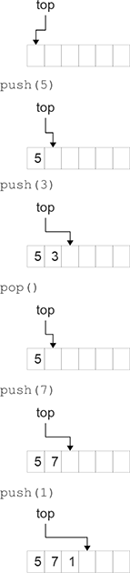
This figure shows a graphical representation of an array-based stack and how it changes over several operations. The stack stores data in the array and uses an integer index to keep track of the position of the top.
Though this figure does not show it, we also need to handle the situation where enough elements have been pushed that the array fills. In this situation, a larger array needs to be allocated and the values should be copied over so that we have room for more elements.
Code that implements this view of a stack can be seen here.
package scalabook.adt
class ArrayStack[A : Manifest] extends Stack[A]{
private var top = 0
private var data = new Array[A](10)
def push(obj:A) {
if(top >= data.length) {
val tmp = new Array[A](data.length∗2)
Array.copy(data,0,tmp,0,data.length)
data = tmp
}
data(top) = obj
top += 1
}
def pop():A = {
assert(!isEmpty,"Pop called on an empty stack.")
top -= 1
data(top)
}
def peek:A = data(top-1)
def isEmpty:Boolean = top==0
}
We will run through this beginning at the top. The class is called ArrayStack and it extends Stack. The ArrayStack takes a type parameter called A that is passed through to Stack. This type parameter is modified in a way we have not seen before, it is followed with : Manifest. This is required for us to be able to make an array of A using new Array[A](...). The details of why this is needed are explained in the advanced section below.
Inside the class we have two private var declarations for top and the array called data. The implementations of pop():A decrements top and returns the data that is there. Both peek and isEmpty are even simpler. All of these methods are clearly O(1) because they do math on an integer and direct access on an array, both operations that occur in constant time.
The only complex method is push(obj:A). This method ends with two lines that actually place the object in the array and increment top. The first part of the method is a check to make sure that there is space to place the object in the array. If there is not, a new array is made and the contents of the current array are copied into the new one, then the reference data is changed to point to the new array. Everything here is O(1) except the call to Array.copy. That call takes O(n) time because it has to move O(n) values from one array to another.
The obvious question is, will this average out to give us an amortized cost of O(1)? For this code, the answer is yes, but it is very important to see why, as it would have been very easy to write a version that has an amortized cost of O(n). The key is in how we grow the array. In this code, every time we need more space, we make the array twice as big. This might seem like overkill, and many would be tempted to instead add a certain amount each time. Perhaps make the array 10 slots bigger each time. The table below runs through the first six copy events using these two approaches. At the bottom it shows generalized formulas for the mth copy event.
To get the amortized cost, we divide the total work by the size because we had to call push that number of times to get the stack to that size. For the first approach we get
.
For the second approach we get
.
Neither the multiple of 2, nor the addition of 10 is in any way magical. Growing the array by a fixed multiple greater than one will lead to amortized constant cost. Growing the array by any fixed value will lead to an amortized linear cost. The advantage of the fixed multiple is that while the copy events gets exponentially larger, they happen inversely exponentially often.
Manifests (Advanced)
To understand Manifests, it helps to have some understanding of the history of Java as the nature of the Java Virtual Machine (JVM) plays a role in their existence. The parallel to Scala type parameters in Java is generics. Generics did not exist in the original Java language. In fact, they were not added until Java 5. At that point, there were a huge number of JVMs installed around the globe and it was deemed infeasible to make changes that would invalidate all of them. For that reason, as well as a motivation to keep the virtual machine fairly simple, generics were implemented using erasure. What this means is that the information for generics was used at compile time, but was erased in the compiled version so that at runtime it was impossible to tell what the generic type had been. In this way, the code that was produced looked like what would have been produced before generics were introduced.
This has quite a few effects on how Java programs are written. It comes through in Scala as a requirement for having a manifest on certain type parameters. The manifest basically holds some of the type information so that it is available at runtime. To understand why we need this, we should go back to the expression that was responsible for us needing a manifest: new Array[A](10). This makes a new Array[A] with 10 elements in it and sets the 10 elements to appropriate default values. It is the last part that leads to the requirement of having a manifest. For any type that is a subtype of AnyRef, the default value is null. For the subtypes of AnyVal, the default varies. For Int, it is 0. For Double it is 0.0. For Boolean it is false. In order to execute that expression, you have to know enough at least enough about the type to put in proper default values.1 Type erasure takes away that information from the runtime. The manifest allows Scala to get back access to it.
It is also worth noting that our implementation of the stack technically does not actually remove the value from the array when pop() is called. This remove is not really required for the stack to execute properly. However, it can improve memory usage and performance, especially if the type A is large. Unfortunately, that would require having a default value to put into the array in that place, which we have just discussed it is hard from a completely general type parameter.
24.6 Array-Based Queue
Like the stack, the code for the array-based queue begins by setting up the ADT as a completely abstract trait. This trait, which takes a type parameter so that it can work with any type, is shown here.
package scalabook.adt
/∗∗
∗ This trait defines a mutable Queue ADT.
∗ @tparam A the type of data stored
∗/
trait Queue[A] {
/∗∗
∗ Add an item to the queue.
∗ @param obj the item to add
∗/
def enqueue(obj:A)
/∗∗
∗ Remove the item that has been on the longest.
∗ @return the item that was removed
∗/
def dequeue():A
/∗∗
∗ Return the item that has been on the longest without removing it.
∗ @return the most recently added item
∗/
def peek:A
/∗∗
∗ Tells whether this queue is empty.
∗ @return true if there are no items on the queue, otherwise false.
∗/
def isEmpty:Boolean
}
As with the stack, this has only the signatures of the methods along with comments describing what they do.
The queue ADT can also be implemented using an array. Figure 24.3 shows how this might look for several operations. Unlike the stack, the queue needs to keep track of two locations in the array: a front and a back. The back is where new elements go when something is added to the queue and the front is where values are taken from when they are removed. Both indexes are incremented during the proper operations. When an index moves beyond the end of the array, it is wrapped back around to the beginning. This allows us to continually add and remove items without having to grow the array or copy elements around. Both of those would require O(n) operations and prevent our total performance from being O(1).

This figure shows a graphical representation of an array-based queue and how it changes over several operations. The queue stores data in the array and uses integer indexes to keep track of the front and back.
This figure does not show what happens when the queue gets full. At that point a bigger array is needed and values need to be copied from the old array into the new one. The details for the queue are not quite as straightforward as they were for the stack. Figure 24.4 demonstrates the problem and a possible solution. Doing a direct copy of elements is not appropriate because the wrapping could have resulted in a situation where the front and back are inverted. Instead, the copy needs to shift elements around so that they are contiguous. The values of front and back need to be adjusted appropriately as well. There are many ways that this could be done. Figure 24.4 demonstrates the approach that we will take in the code here where the front is moved back to the beginning of the array.
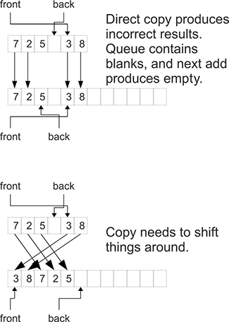
This figure shows a graphical representation of an array-based queue when it needs to grow on an enqueue. The queue is seen as empty if front==back. For that reason, the grow operation should happen when the last slot will be filled. In addition to growing a bigger array, the copy operation needs to move elements of the array around and alter the location of front and back.
This graphical description of implementing an array-based queue can be implemented in code like the following.
package scalabook.adt
class ArrayQueue[A : Manifest] extends Queue[A] {
private var front,back = 0
private var data = new Array[A](10)
def enqueue(obj:A) {
if((back+1)%data.length==front) {
val tmp = new Array[A](data.length∗2)
for(i <- 0 until data.length-1) tmp(i) = data((i+front)%data.length)
front = 0
back = data.length-1
data = tmp
}
data(back) = obj
back = (back+1)%data.length
}
def dequeue():A = {
assert(!isEmpty,"Dequeue called on an empty queue.")
val ret = data(front)
front = (front+1)%data.length
ret
}
def peek:A = data(front)
def isEmpty:Boolean = front==back
}
This code is very similar to what we had for the stack. The only element that you might find odd is that the wrapping from the end of the array back to the beginning is done with a modulo. The wrap in dequeue and the one at the end of enqueue could easily be done with an if. For the other two, the wrapping needs to be part of an expression. This makes the modulo far more effective.
All the operations have an amortized cost of O(1). As with push on the stack, the dequeue method will be O(n) on the calls where it has to grow. However, those are rare enough that they average out to constant time.
24.7 Unit Tests
As you are well aware by this time, writing code that compiles does mean that you have code that is correct. There can still be runtime and logic errors present in the code. In order to find these you need to test the code. The topic of testing was first addressed back in section 8.5. The tests described at that point were manual tests. Each test had to be run explicitly by the developer if we wanted to test the code. In addition, some of the tests would print values that had to be verified for correctness by the programmer. In large-scale development, these approaches fall short of helping us to produce reliable code. In this section we will address this by introducing the concept of automated unit tests.
A unit test is a test that checks the functionality of some particular unit of a program. Typically it is something like a single class or even some methods in a class. The unit test is intended to be run automatically and, as such, does not rely on programmer interaction to determine if the test passed or failed. That logic should be built into the test. This allows unit tests to be run frequently. The idea is that every time you make changes to the code, you rerun all the unit tests to make sure that the changes did not break anything.
There are many types of unit-testing frameworks. Some, such as ScalaTest, ScalaCheck, and Specs, have been written specifically for Scala. In this book we will use JUnit, the primary unit-testing framework for Java. The reasons for this choice include the fact that JUnit is broadly used, it is easy to use, and it has support built into Eclipse and other IDEs.
24.7.1 Setup
There are a few steps that we need to take to get JUnit running with our project in Eclipse. First, go to http://www.junit.org/ and click on "Download JUnit". That will take you to a page with many different downloads. You should get the newest release of the "Basic jar". Save this file in your Eclipse workspace or some other location where it will be easy to find.
Now go into Eclipse and right click on the project you want to add testing to. From the pop-up menu, select "Build Path" > "Configure Build Path...". Go to the "Libraries" tab and click on "Add External JARs..." button. After you have navigated to the file and selected it you are done setting up that project to run JUnit tests.
24.7.2 Writing Tests
Unlike tests that we would put in a main method in a companion object, unit tests are put in separate files and even in separate packages or projects. We will take the approach of putting all test code in a parallel package hierarchy that begins with test. As the ArrayStack and ArrayQueue were in the scalabook.adt package, our tests will be in test.scalabook.adt. To make the tests we simply write classes with methods and annotate our test methods with the @Test annotation from JUnit. For that to compile you should do an import for org.junit. _. Every method that you put the @Test annotation on will be run at part of the unit testing.
Inside of the test methods, you need to have calls to JUnit assert methods. There are methods such as assertTrue, assertFalse, and assertEquals. Typically, tests are written building up from those that test very simple requirements to more significant ones. To understand how simple, consider the following examples.
@Test def emptyOnCreate {
val stack = new ArrayStack[Int]
assertTrue(stack.isEmpty)
}
@Test def nonEmptyOnPush {
val stack = new ArrayStack[Int]
stack.push(5)
assertFalse(stack.isEmpty)
}
@Test def pushPop {
val stack = new ArrayStack[Int]
stack.push(5)
assertEquals(5,stack.pop)
}
The first two only check that a new stack is empty and that after something has been pushed it is not empty. It is not until the third test that we even pop the stack and check that we get back the correct value.
You should notice that all of these methods begin with the same line. Code duplication like this is frowned on in testing as much as it is in normal code development. However, because JUnit runs every test separately, you have to use a tag to make sure that the code you want to run happens before each and every test. The tag for this purpose is the @Before tag. If you have code that needs to follow every test to clean up after something that happens in the "before" method, there is also a @After tag. You can see these used, along with a more complete set of tests for the ArrayStack in this code.
package test.scalabook.adt
import org.junit._
import org.junit.Assert._
import scalabook.adt._
class TestArrayStack {
var stack:Stack[Int] = null
@Before def initStack {
stack = new ArrayStack[Int]
}
@Test def emptyOnCreate {
assertTrue(stack.isEmpty)
}
@Test def nonEmptyOnPush {
stack.push(5)
assertFalse(stack.isEmpty)
}
@Test def pushPop {
stack.push(5)
assertEquals(5,stack.pop)
}
@Test def pushPopPushPop {
stack.push(5)
assertEquals(5,stack.pop)
stack.push(3)
assertEquals(3,stack.pop)
}
@Test def pushPushPopPop {
stack.push(5)
stack.push(3)
assertEquals(3,stack.pop)
assertEquals(5,stack.pop)
}
@Test def push100Pop100 {
val nums = Array.fill(100)(util.Random.nextInt)
nums.foreach(stack.push(_))
nums.reverse.foreach(assertEquals(_,stack.pop))
}
}
These tests are incomplete. It is left as an exercise for the student to come up with and implement additional tests.
With these tests written now we just need to run them and make certain that our implementation passes all the tests. If you select a run option for that file in Eclipse, you should have an option for "JUnit Test". If you select that, you should see something similar to what is shown in figure 24.5. This shows the six tests from above all passing. When everything passes, we get a green bar. If any tests fail there would be a red bar and the tests that fail would be shown in red. You can click on failed tests to find out what assert caused them to fail.
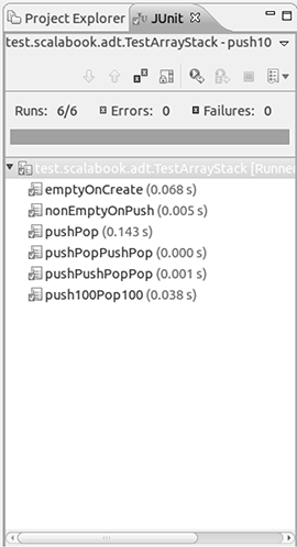
This is what Eclipse shows when a JUnit test is run and all tests are passed. A green bar means that everything is good. If you get a red bar then one or more tests have failed and they will be listed for you.
Similar tests can be written for our queue. They might look like the following.
package test.scalabook.adt
import org.junit._
import org.junit.Assert._
import scalabook.adt._
class TestArrayQueue {
var queue:Queue[Int] = null
@Before def initQueue {
queue = new ArrayQueue[Int]
}
@Test def emptyOnCreate {
assertTrue(queue.isEmpty)
}
@Test def nonEmptyOnEnqueue {
queue.enqueue(5)
assertFalse(queue.isEmpty)
}
@Test def enqueueDequeue {
queue.enqueue(5)
assertEquals(5,queue.dequeue)
}
@Test def enqueueDequeueEnqueueDequeue {
queue.enqueue(5)
assertEquals(5,queue.dequeue)
queue.enqueue(3)
assertEquals(3,queue.dequeue)
}
@Test def enqueueEnqueueDequeueDequeue {
queue.enqueue(5)
queue.enqueue(3)
assertEquals(5,queue.dequeue)
assertEquals(3,queue.dequeue)
}
@Test def enqueue100Dequeue100 {
val nums = Array.fill(100)(util.Random.nextInt)
nums.foreach(queue.enqueue(_))
nums.foreach(assertEquals(_,queue.dequeue))
}
}
You can check these as well and see that our array-based implementation of a queue passes all of these tests.
24.7.3 Test Suites
The purpose of automated testing is to make it easy to run all the tests regularly during development. Having the ability to run all of your tests on a regular basis makes you more confident when you go to make changes to your code. If you run the tests and they pass, then make a change and one or more fail, you know exactly what caused the failure and it will be easier to locate and diagnose.
Unfortunately, going through every test class and running it would be just as much of a pain as going through a large number of objects that have a main defined for testing. To consolidate your test runs, you can make a test suite. This lets you specify a group of different classes that contain test code that should be run together. To build a test suite you make a class and annotate it with the @RunWith and @Suite.SuiteClasses annotations. Here is an example of a suite that contains the two tests we just wrote.
package test
import org.junit.runner.RunWith
import org.junit.runners.Suite
@RunWith(classOf[Suite])
@Suite.SuiteClasses(Array(
classOf[scalabook.adt.TestArrayStack],
classOf[scalabook.adt.TestArrayQueue],
classOf[scalabook.util.TestRPNCalc]
))
class AllTests
Note that the class does not actually contain anything at all. It is the annotations that tell JUnit all the work that should be done here. As we add more test classes, we will also add them to our suite.
24.7.4 Test-Driven Development
Unit tests are a central part of an approach to development called "Test Driven Development" (TDD). This style of development is highlighted by the idea that you write tests for code before you write the actual code. In a TDD environment, a programmer who wants to write a new class would create the class and put in blank methods which have just enough code to get the class to compile. Methods that return a value are set to return default values such as null, 0, or false. No logic or data is put in.
After that, the developer writes a basic test for the class and runs the test to see that it fails. Then just enough code is added to make that test pass. Once all existing tests pass, another test is written which fails and this process is repeated until a sufficient set of tests have been written to demonstrate that the class must meet the desired requirements in order to pass them all.
While the textbook does not follow a TDD approach, there are some significant benefits to it. The main one is that it forces a developer to take small steps and verify that everything works on a regular basis. It also gives you a feeling of security when you are making changes because generally feeling confident that if you make a change which breaks something, it will immediately manifest as a red bar in testing. This can be important for novice programmers who often leave large sections of code in comments because they are afraid to delete them in case something goes wrong. For this reason, the literature on TDD refers to tests as giving you the "courage" to make changes.
There is a lot more to unit testing that we have not covered here. Interested readers are encouraged to look at the JUnit website or look into Scalabased testing frameworks such as ScalaCheck and ScalaTest. Full development needs more than just unit testing as well. Unit tests, by their nature, insure that small pieces of code work alone. To feel confident in a whole application, you need to test the parts working together. This is called integration testing and it too is done on a fairly regular basis in TDD.
24.8 RPN Calculator
A classic example usage of a stack is the Reverse Polish Notation (RPN) calculator. In RPN mode, operations are entered after the values that they operate on. This is also called post-fix notation. The RPN representation of "2 + 3" is "2 3 +" While this might seem like an odd way to do things, it has one very significant advantage, there is no need for parentheses to help specify order of operation. Using standard notation, also called in-fix notation, the expressions "2 + 3 ∗ 5" and "5 ∗ 3 + 2" are both 17 because multiplication occurs before addition, regardless of the order things are written. If you want the addition to happen first, you must specify that with parentheses, "(2 + 3) ∗ 5". Using post-fix notation, we can say "3 5 ∗ 2 +" to get 17 or "2 3 + 5 ∗" if we want the addition to happen first so we get 25. This lack of parentheses can significantly reduce the length of complex expressions which can be appealing when working on such things.
The evaluation of a post-fix expression can be done quite easily with a stack that holds the numbers being worked with. Simply run through the expression and for each element you do one of the following. If it is a number, you push that number onto the stack. If it is an operator, you pop two elements front the stack, perform the proper operation on them, and then push the result back on the stack. At the end there should be one value on the stack which represents the final result. We could implement this basic functionality using the following object.
object RPNCalc {
def apply(args:Seq[String]):Double = {
val stack = new ArrayStack[Double]
for(arg <- args; if(arg.nonEmpty)) arg match {
case "+" => stack.push(stack.pop+stack.pop)
case "∗" => stack.push(stack.pop∗stack.pop)
case "-" => val tmp = stack.pop; stack.push(stack.pop-tmp)
case "/" => val tmp = stack.pop; stack.push(stack.pop/tmp)
case x => stack.push(x.toDouble)
}
stack.pop
}
}
These arguments are passed in as a sequence that is traversed using a for loop. The subtract and divide operators are slightly different from those for addition and multiplication simply because they are not commutative, the order of their operands matters. This code also assumes that anything that is not one of the four operators is a number.
There are a few options that would be nice to add to this basic foundation. For example, it would be nice to have a few other functions beyond that standard four arithmetic operations. It would also be nice to have support for variables so that not every value has to be a literal numeric value. A final object that supports these additions is shown here.
package scalabook.util
import scalabook.adt.ArrayStack
object RPNCalc {
def apply(args:Seq[String],vars:collection.Map[String,Double]):Double = {
val stack = new ArrayStack[Double]
for(arg <- args; if(arg.nonEmpty)) arg match {
case "+" => stack.push(stack.pop+stack.pop)
case "∗" => stack.push(stack.pop∗stack.pop)
case "-" => val tmp = stack.pop; stack.push(stack.pop-tmp)
case "/" => val tmp = stack.pop; stack.push(stack.pop/tmp)
case "sin" => stack.push(math.sin(stack.pop))
case "cos" => stack.push(math.cos(stack.pop))
case "tan" => stack.push(math.tan(stack.pop))
case "sqrt" => stack.push(math.sqrt(stack.pop))
case v if(v(0).isLetter) => stack.push(try {vars(v)} catch {case ex => 0.0
})
case x => stack.push(try {x.toDouble} catch {case ex => 0.0})
}
stack.pop
}
}
This has added the three main trigonometric functions along with a square root function. These operations pop only a single value, apply the function, and push back the result. This code also includes an extra argument of type Map[String,Double] to store variables by name. In this case, the scala.collection.Map type is used. This is a supertype to both the mutable and immutable maps. This code does not care about mutability so this provides additional flexibility. Lastly, some error handling was added so that if a value comes in that is neither a number, nor a valid variable, we push 0.0 to the stack.
Before we can proclaim that this code works, we need to test it.2 Here is a possible test configuration.
package test.scalabook.util
import org.junit._
import org.junit.Assert._
import scalabook.util.RPNCalc
class TestRPNCalc {
@Test def basicOps {
assertEquals(5,RPNCalc("2 3 +".split(" "),null),0.0)
assertEquals(6,RPNCalc("2 3 ∗".split(" "),null),0.0)
assertEquals(3,RPNCalc("6 2 /".split(" "),null),0.0)
assertEquals(1,RPNCalc("3 2 -".split(" "),null),0.0)
}
@Test def twoOps {
assertEquals(20,RPNCalc("2 3 + 4 ∗".split(" "),null),0.0)
assertEquals(3,RPNCalc("2 3 ∗ 3 -".split(" "),null),0.0)
assertEquals(5,RPNCalc("6 2 / 2 +".split(" "),null),0.0)
assertEquals(0.25,RPNCalc("3 2 - 4 /".split(" "),null),0.0)
}
@Test def vars {
val v = Map("x" -> 3.0, "y" -> 2.0)
assertEquals(20,RPNCalc("2 x + 4 ∗".split(" "),v),0.0)
assertEquals(3,RPNCalc("y 3 ∗ x -".split(" "),v),0.0)
assertEquals(5,RPNCalc("6 2 / y +".split(" "),v),0.0)
assertEquals(0.25,RPNCalc("x y - 4 /".split(" "),v),0.0)
}
@Test def specials {
val v = Map("pi" -> 3.14159, "x" -> 3.0, "y" -> 2.0)
assertEquals(0,RPNCalc("pi cos 1 +".split(" "),v),1e-8)
assertEquals(math.sqrt(2)+3,RPNCalc("y sqrt x +".split(" "),v),1e-8)
assertEquals(1,RPNCalc("pi 2 / sin".split(" "),v),1e-8)
assertEquals(0.0,RPNCalc("x y y 2 / + - tan".split(" "),v),1e-8)
}
}
As with the earlier tests, these are fairly minimal. There are literally an infinite number of tests that could be run to verify the RPN calculator. This set simply picks a few different tests related to the different types of functionality the calculator is supposed to support.
True unit testing adherents would prefer that each assertEquals be split into a separate method because none depends on the results before it. This is not just a style issue either, there are valid functionality benefits to that approach. JUnit will run all the test methods independently, but each test method will stop when an assert fails. So if the processing of "2 3 +" were to fail, we would not get results from the other three lines of that test as it is written now. That makes it harder to know why it failed. If "2 3 +" fails and all the other single operator calls pass, we can feel fairly confident the problem is with the handling of "+". As it is written now, we will not get that extra information. The only reason for using the format shown here is that it takes less than half as many lines to make this readable.
This RPNCalc object can also be integrated into the drawing program as a command. To make use of the variables, we add an extra val to the Drawing class called vars that is a mutable.Map[String,Double]. Then we add two commands called "rpn" and "set". The first invokes that RPNCalc object with the specified arguments. The second allows you to set variables in the Map for that drawing. Here is code for the modified version of Commands
package scalabook.drawing
/∗∗
∗ This object defines the command processing features for the drawing.
∗ Use apply to invoke a command.
∗/
object Commands {
private val commands = Map[String,(String,Drawing)=>Any](
"add" -> ((rest,d) => rest.trim.split(" +").map(_.toInt).sum),
"echo" -> ((rest,d) => rest.trim),
"refresh" -> ((rest,d) => d.refresh),
"freeze" -> ((rest,d) => Thread.sleep(rest.trim.toInt∗1000)),
"rpn" -> ((rest,d) => scalabook.util.RPNCalc(rest.trim.split(" +"),d.vars)),
"set" -> ((rest,d) => {
val parts = rest.trim.split(" +")
d.vars(parts(0)) = parts(1).toDouble
parts(0)+" = "+parts(1)
})
)
def apply(input:String,drawing:Drawing):Any = {
val spaceIndex = input.indexOf(‘ ‘)
val (command,rest) = if(spaceIndex < 0) (input.toLowerCase(),"")
else (input.take(spaceIndex).toLowerCase(),input.drop(spaceIndex))
if(commands.contains(command)) commands(command)(rest,drawing)
else "Not a valid command."
}
}
Thanks to the flexibility of the original design, there is very little effort required for adding two additional commands. More effort was required to add vars to Drawing. The obvious addition is in the top line where arguments are passed in.
class Drawing(private val root:DrawTransform,private[drawing] val
vars:mutable.Map[String,Double]) extends Serializable {
The greater challenge comes from the fact that the apply method in the companion object that deserializes XML needs to be given an appropriate map. Here is code for the two versions of apply and the one method that builds a map from XML.
def apply(data:xml.Node):Drawing = {
new Drawing(DrawTransform(null,(data "drawTransform")(0)),buildVars(data
"variable"))
}
def apply():Drawing = {
new Drawing(new DrawTransform(null),mutable.Map[String,Double]())
}
def buildVars(nodes:NodeSeq):mutable.Map[String,Double] = {
mutable.Map((for(n <- nodes) yield (n "@name").text -> (n
"@value").text.toDouble):_∗)
}
To pull the data out of the XML means that it has to get there in the first place. For this reason, we must also alter the toXML method in Drawing to include extra elements for the variables. This can be done with the following code.
def toXML : xml.Node =
<drawing>
{root.toXML}
{for((n,v) <- vars) yield (<variable name={n} value={v.toString}/>)}
</drawing>
A for loop is used here to simplify the syntax of dealing with the tuples that come out of the map.
24.9 End of Chapter Material
24.9.1 Summary of Concepts
- The term Abstract Data Type, ADT, is used to describe a programmatic structure that has well-defined operations, but that does not specify how those operations are carried out. This concept links back to the ideas of separation of interface and implementation.
- A stack is a simple ADT with two basic operations, push and pop. The push operation adds an element to the top of the stack. The pop operation removes the most recently added element. This order of content removal is called Last In First Out, LIFO.
- A queue is another simple ADT with enqueue and dequeue operations. The enqueue adds an element to a queue while the dequeue takes out the element that has been in the queue the longest. This ordering scheme for removal of elements is called First In First Out, FIFO.
- Order analysis helps us understand the way in which algorithms behave as input sizes get larger. The O notation ignores constant multiples and lower-order terms. It is only really relevant when the input sizes get large.
- Due to their simplicity, any reasonable implementation of a stack or a queue should have operations that have an O(1) amortized cost.
- One way to implement that stack ADT is using an Array to store the data. Simply keep an index to the top of the stack in the Array and build up from 0. When the Array is full, it should be grown by a multiplicative factor to maintain O(1) amortized cost over copying operations.
- It is also possible to implement a queue with an Array. The implementation is a bit more complex because data is added at one end of the queue and removed at the other. The front and back are wrapped around when they hit the end so the Array stays small and no copies are needed for most operations. Like the stack, when the Array does have to grow, it should do so by a multiplicative factor.
- Testing is a very important part of software development. Unit Tests are tests of the functionality of small units of code, such as single classes. The JUnit framework provides a simple way of building unit tests that can be run regularly during software development.
24.9.2 Exercises
- Add extra functions to the RPN calculator.
- Write more tests for the JUnit tests that are shown in the book.
- Write some code so that requests that are sent across a network are queued up and handled in the order they arrive. You can simulate a long-running calculation with Thread.sleep.
- For this exercise you should implement a few possible versions of both the queue and the stack and then perform timing tests on them to see how well they scale. You will include the implementation that we developed in this chapter plus some slightly modified implementations to see how minor choices impact the final speed of the implementation.
- Build your own version of BlockingQueue using synchronized, wait, and notifyAll to reproduce the behavior of the version in java.util.concurrent.
24.9.3 Projects
As you can probably guess, the projects for this chapter have you adding stacks and/or queues to your code. A number of them have you making thread-safe queues to put into your code in places you might have been using a java.util.concurrent.BlockingQueue.
-
If you have been working on the MUD project, for this iteration you should make your own thread-safe queue, specifically for handing players who have logged in from the server socket thread to the main game thread. You can decide exactly what functionality to include, but the two critical aspects are that it needs to be a FIFO and thread-safe.
-
If you have been working on the web spider project, make and use your own threadsafe queue for handing information between the socket reading threads and the parsing threads and back. There will be at least two instances of queues for these functions with at least one for each direction of data flow.
-
If you are working on a networked graphical game you need to write a thread-safe queue for the same purposes as that needed for the MUD.
-
Back in project 4 (p.494) on the math worksheet it was suggested that you could integrate polymorphism into your project by using the command pattern. One of the main uses of the command pattern is to implement undo and redo capabilities. A stack is an ideal data structure for doing this. You have the main application keep track of two stacks. One is the undo stack, which you push commands onto as they are executed. When the user selects to undo something, you pop the last command on the undo stack, call its undo method, then push it to a second stack, which is a redo stack. When a user selects redo, things move in the opposite direction. Note that any normal activity should probably clear the redo stack.
The stack that you use for this will probably be a bit different from the default implementation. For one thing, you need the redo stack to have a clear method. In addition, you might not want unlimited undo so you might want the stack to "lose" elements after a certain number have been pushed. It is left as an exercise for the student to consider how this might be implemented in a way that preserves O(1) behavior.
-
Project 5 (p.494) suggested that you add the command pattern to the Photoshop® project in order to implement undo and redo capabilities. As was described in the project above, this is best done with two stacks. For this iteration you should do for Photoshop what is described above for the math worksheet.
-
So far the projects for the simulation workbench have had you working with N-body simulations like gravity or a cloth particle-mesh. Now we want to add a fundamentally different type of simulation to the mix, discrete event simulations. These are discussed in more depth in chapter 26, but you can create your first simple one here, a single-server queue.
The idea of a single-server queue is that you have people arriving and getting in line to be receiving service from a single server. The people arrive at random intervals and the server takes a random amount of time to process requests. When people arrive and the server is busy, they enter a queue. The simulation can keep track of things like how long people have to wait and the average length of the queue.
The key to a discrete event simulation is that all you care about are events, not the time in between. In this system, there are only two types of events, a customer arriving and a service being completed. Only one of each can be scheduled at any given time. To model arrivals you will use an exponential distribution and to model service times you will use a Weibull distribution. The following formulas can be used to generate numbers from these distributions, where r is the result of a call to math.random.
For the Weibull, use k = 2. The λ values determine the average time between arrivals or services. You should let the user alter those.
The simulation should start at t = 0 with no one in the queue. You generate a value from the exponential distribution, aexponential,1 and instantly advance to that time, when the first person enters. As no one is being served at that time, they go straight to the server. You also generate another number from the exponential distribution, aexponential,2 and keep that as the time the next person will enter. The first person going to the server causes you to generate a service time, aWeibull,1 for when that person will finish the service, and you store that.
You then instantly advance to the lower of the two event times. So either a second person arrives and enters the queue, or the first person is serviced and the server becomes free with no one present. Each time one person arrives, you schedule the next arrival. Each time a person goes to the server, you schedule when they will be done. Note that the generated times are intervals so you add them to the current time to get when the event happens.
Let the user determine how long to run the simulation. Calculate and display the average wait time, the average line length, and the fraction of time the server is busy.
-
For non-networked games, it is hard to predict what will fit well. For some you can implement undo and redo functionality as described in project 4. That applies best to turn-based games. It is also possible that you can find places where queues can be used to pass information between threads or to queue up commands from the user if there are delays on how long actions take.
1 You also need other information such as how big a memory block should be reserved. For example, Int requires 4-bytes while Double requires 8.
2 It is worth noting that there was a bug in this code originally that was caught by these tests.