Chapter 6

Recursion for Iteration

Gaining conditionals provided us with a lot of power. We are now able to express logic in our code. Adding functions gave us the ability to break problems into pieces and repeat functionality without retyping code. There is still something very significant that we are missing. Now when we write a piece of logic, it happens once. We can put that logic into a function and then call the function over and over, but it will only happen as many times as we call it. We can not easily vary the number of times that something happens. There is more than one way to make something happen multiple times in Scala. One of these ways, recursion, we can do with just functions and conditionals, constructs that we have already learned.

6.1 Basics of Recursion

Recursion is a concept that comes from mathematics. A mathematical function is recursive if it is defined in terms of itself. To see how this works, we’ll begin with factorial. You might recall from math classes that n! is the product of all the integers from 1 up to n. We might write this as n! = 1 * 2 * ... * n. More formally we could write it like this.

$n!={\displaystyle \prod _{i=1}^{n}i}$

Both of the formal and informal approaches define factorial in terms of just multiplication, and assume that we know how to make that multiplication happen repeatedly. We can be more explicit about the repetition if we write the definition using recursion like this.

$n!=\{\begin{array}{ll}1\hfill & n<2\hfill \\ n*(n-1)!\hfill & otherwise\hfill \end{array}$

In this definition, the factorial function is defined in terms of itself. To describe what factorial is, we use factorial.

To see how this works, let us run through an example and take the factorial of 5. By our definition we get that 5! = 5 * 4!. This is because 5 is not less than 2. Subsequently, we can see that 4! = 4 * 3! so 5! = 5 * 4 * 3!. This leads to 5! = 5 * 4 * 3 * 2! and finally to 5! = 5 * 4 * 3 * 2 * 1.

This definition and its application illustrate two of the key aspects of recursion. There are two possibilities for the value of this function. Which one we use depends on the value of n. In the case where n is less than 2, the value of the factorial is 1. This is called a base case. All recursive functions need some kind of base case. The critical thing about a base case is that it is not recursive. When you get to a base case, it should have a value that can be calculated directly without reference back to the function. Without this you get what is called infinite recursion. There can be multiple different base cases as well. There is no restriction that there be only one, but there must be at least one.

To see why the base case is required, consider what would happen without it. We would still get 5! = 5 * 4 * 3 * 2!, but what would happen after that? Without a base case, 2! = 2 * 1!. Technically there is not a problem there, but what about 1!? 1! = 1 * 0! in the absence of a base case and 0! = 0 * (−1)!. This process continues on forever. That is why it is called infinite recursion.

The second case of the recursive definition demonstrates the recursive case. Not only does this case refer back to the function itself, it does so with a different value and that value should be moving us toward a base case. In this case, we define n! In terms of (n – 1)!. If the recursive case were to use the same value of n we would have infinite recursion again. Similarly, if it used a value greater than n we would also have infinite recursion because our base case is for small numbers, not large numbers.

What else could we define recursively? We could define multiplication, which is used by factorial, recursively. After all, at least for the positive integers, multiplication is nothing more than repeated addition? As with the factorial, we could write a definition of multiplication between positive integers that uses a math symbol that assumes some type of repetition like this.

$m*n={\displaystyle \sum _{i=1}^{n}m}$

This says that m*n is m added to itself n times. This can be written as a recursive function in the following way.

$m*n=\{\begin{array}{ll}0\hfill & n=0\hfill \\ m+m*(n-1)\hfill & otherwise\hfill \end{array}$

This function has two cases again, with a base case for a small value and a second, recursive case, that is defined in terms of the value we are recursing using a smaller value of that argument.

We could do the same type of things to define exponentiation in terms of multiplication. We could also use an increment (adding 1) to define addition by higher numbers. It is worth taking a look at what that would look like.

$m+n=\{\begin{array}{ll}m\hfill & n=0\hfill \\ 1+m+(n-1)\hfill & otherwise\hfill \end{array}$

While this seems a bit absurd, it would be less so if we named our functions. Consider the following alternate way of writing this.

$add(m,n)=\{\begin{array}{ll}m\hfill & n=0\hfill \\ 1+add(m,n-1)\hfill & otherwise\hfill \end{array}$

Now it is clear that as long as we can do increment (+1) and decrement (-1) we could write full addition. With full addition we could write multiplication. With multiplication we can write exponentiation or factorial. It turns out that this is not all you can do. It might be hard to believe, but if you have variables, recursion (which simply requires functions and an if construct), increment, and decrement, you have a full model of computation. It can calculate anything that you want. Of course, we do not do it that way because it would be extremely slow. Still, from a theoretical standpoint it is very interesting to know that so much can be done with so little.

6.2 Writing Recursion

We have seen the mathematical side of recursion and have written some basic mathematical functions as recursive functions. Now we need to see how we write these things and more in Scala. The translation from math functions to programming functions is not hard. In fact, little will change from the math notation to the Scala notation.

As before, we will begin with the factorial function. Here is the factorial function written in Scala in the REPL.

scala> def fact(n:Int):Int = if(n<2) 1 else n*fact(n-1)

fact: (n: Int)Int

We have called the function fact, short for factorial. The body of the function is a single if expression. First it checks the value of n to see if it is less than 2. If it is, the expression has a value of 1. Otherwise it is n*fact(n-1). We can see the results of using this function here:

scala> fact(5)

res1: Int = 120

We see here that it correctly calculates the factorial of 5.

One significant difference between recursive and non-recursive functions in Scala is that we have to specify the return type of recursive functions. If you do not, Scala will quickly let you know it is needed.

scala> def fact(n:Int) = if(n<2) 1 else n*fact(n-1)

<console>:6: error: recursive method fact needs result type

  def fact(n:Int) = if(n<2) 1 else n*fact(n-1)

         ^

Factorial is an interesting function that is significant in Computer Science when we talk about how much work certain programs have to do. Some programs have to do an amount of work that scales with the factorial of the number of things they are working on. We can use our factorial function to see what that would mean. Let us take the factorial of a few different values.

scala> fact(10)

res2: Int = 3628800

scala> fact(15)

res3: Int = 2004310016

scala> fact(20)

res4: Int = -2102132736

The first two show you that the factorial function grows very quickly. Indeed, programs that do factorial work are referred to as intractable because you can not use them for even modest-size problems. The third example though shows something else interesting. The value of 20! should be quite large. It certainly should not be negative. What is going on here?

If you remember back to chapter 3, we talked about the way that numbers are represented on computers. Integers on computers are represented by a finite number of bits. As a result, they can only get so large. The built in number representations in Scala use 32 bits for Int. If we changed our function just a bit to use Long we could get 64 bits. Let’s see that in action.

scala> def fact(n:Long):Long = if(n<2) 1L else n*fact(n-1)

fact: (n: Long)Long

scala> fact(20)

res5: Long = 2432902008176640000

scala> fact(30)

res6: Long = -8764578968847253504

The 64 bits in a Long are enough to store 20!, but they still fall short of 30!. If we give up the speed of using the number types hard wired into the computer, we can represent much larger numbers. We can then be limited by the amount of memory in the computer. That is a value not measured in bits, but in billions of bytes. To do this, we use the type BigInt.

The BigInt type provides us with arbitrary precision arithmetic. It does this at the cost of speed and memory. You do not want to use BigInt unless you really need it. However, it can be fun to play with using a function like factorial which has the possibility of getting quite large. Let us redefine our function using this type and see how it works.

scala> def fact(n:BigInt):BigInt = if(n<2) 1L else n*fact(n-1)

fact: (n: BigInt)BigInt

scala> fact(30)

res7: BigInt = 265252859812191058636308480000000

scala> fact(150)

res8: BigInt = 571338395644585459047893286526105400318955357860112641

825483758331798291248453983931265744886753111453771078787468542041626

662501986845044663559491959220665749425920957357789293253572904449624

724054167907221184454371222696755200000000000000000000000000000000000

00

Not only can this version take the factorial of 30, it can go to much larger values as you see here. There are not that many applications that need these types of numbers, but they can certainly be fun to play with.

Now that we have beaten factorial to death, it is probably time to move on to a different example. The last section was all about examples pulled from mathematics. The title of this chapter though is using recursion for iteration. This is a far broader programming concept than the mathematical functions we have talked about. So let us use an example that is very specific to programming.

A simple example to start with is to write a function that will “count” down from a certain number to zero. By count here we it will print out the values. Like the factorial we will pass in a single number, the number we want to count down from. We also have to have a base case, the point where we stop counting. Since we are counting down to zero, if the value is ever below zero then we are done and should not print anything.

In the recursive case we will have a value, n, that is greater than or equal to zero. We definitely want to print n. The question is, what do we do after that? Well, if we are counting down, then following n we want to have the count down that begins with n-1. Indeed, this is how you should imagine the recursion working. Counting down from n is done by counting the n, then counting down from n-1. Converting this into code looks like the following:

def countDown(n:Int) {

 if(n>=0) {

 println(n)

 countDown(n-1)

}

}

The way this code is written, the base case does nothing so we have an if statement that will cause the function to simply return if the value of n is less than 0. You can call this function passing in different values for n to verify that it works.

Now let us try something slightly different. What if I want to count from one value up to another? In some ways, this function looks very much like what we already wrote. There are some differences though. In the last function we were always counting down to zero so the only information we needed to know was what we were counting from. In this case though, we need to be told both what we are counting from and what we are counting to. That means that our function needs two parameters passed in. A first cut at this might look like the following.

def countFromTo(from:Int,to:Int) {

 println(from)

 if(from!=to) {

 countFromTo(from+1,to)

}

}

This function will work fine under the assumption that we are counting up. However, if you call this with the intention of counting down so that from is bigger than to, you have a problem. To see why, let us trace through this function. First, let us see what happens if we call it with 2 and 5, so we are trying to count up from 2 to 5. What we are doing is referred to as tracing the code. It is the act of running through code to see what it does. This is an essential ability for any programmer. After all, how can you write code to complete a given task if you are not able to understand what the code you write will do? There are lots of different approaches to tracing. Many involve tables where you write down the values of different variables. For recursive functions you can often just write down each call and what it does, then show the calls it makes. That is what we will do here. We will leave out the method name and just put the values of the arguments as that is what changes.

(2,5) => prints 2

 ↓

(3,5) => prints 3

 ↓

(4,5) => prints 4

 ↓

(5,5) => prints 5

The last call does not call itself because the condition from!=to is false.

Now consider what happens if we called this function with the arguments reversed. It seems reasonable to ask the function to count from 5 to 2. It just has to count down. To see what it will do though we can trace it.

(5,2) => prints 5

 ↓

(6,2) => prints 6

 ↓

(7,2) => prints 7

 ↓

(8,2) => prints 8

 ↓

...

This function will count for a very long time. It is not technically infinite recursion because the Int type only has a finite number of values. Once it counts above 231 – 1 it wraps back around to –231 and counts up from there to 2 where it will stop. You have to be patient to see this behavior though. Even if it is not infinite, this is not the behavior we want. We would rather the function count down from 5 to 2. The question is, how can we do this? To answer this we should go back to the trace and figure out why it was not doing that in the first place.

Looking at the code and the trace you should quickly see that the problem is due to the fact that the recursive call is passed a value of from+1. So the next call is always using a value one larger than the previous one. What we need is to use +1 when we are counting up and -1 when we are counting down. This behavior can be easily added by replacing the 1 with an if expression. Our modified function looks like this.

def countFromTo(from:Int,to:Int) {

 println(from)

 if(from!=to) {

 countFromTo(from+(if(from<to) 1 else -1),to)

}

}

Now when the from value is less than the to value we add 1. Otherwise we will add -1. Since we do not get to that point if the two are equal, we do not have to worry about that situation. You should enter this function in and test it to make sure that it does what we want.

6.3 User Input

We are still limited in what we can realistically do because we are stuck using values that we can easily calculate. For example, we can go from one number to the one before it or the one after. We could use those values as inputs to more complex functions, but we still need them to be calculated from numbers we can nicely iterate through. These are shortcomings that will be fixed in the next chapter. For now, we can look at how to make the user (or more generally standard input) into a source of more interesting values.

We saw back in chapter 3 that we can call the function readInt to read an integer from standard input. Now we want to read multiple values and do something with them. We will start by taking the sum of a specific number of values. We can write a function called sumInputInts. We will pass this function an integer that represents how many integers we want the user to input and it will return the sum of those values. How can we define such a function recursively? Well, if we want to sum up 10 numbers, we could say that sum is the first number, plus the sum of 9 others. The base case here is that if the number of numbers we are supposed to sum gets below 1, then the sum is zero. Let us see what this would look like in code.

def sumInputInts(num:Int):Int = {

 if(num>0) {

 readInt()+sumInputInts(num-1)

} else {

 0

}

}

The if is being used as an expression here. It is the only expression in the function so it is the last one, and it will be the return value of the function. If num, the argument to the function, is not greater than zero, then the function returns zero. If it is, the function will read in a new value and return the sum of that value and what we get from summing one fewer values.

What if we don’t know in advance how many values we are going to sum? What if we want to keep going until the end is reached? We could do this. One problem is determining what represents the end. We need to have the user type in something distinctly different that tells us they have entered all the values they want to sum. An easy way to do this would be to only allow the user to sum positive values and stop as soon as a non-positive value is entered. This gives us a function that does not take any arguments. We do not have to tell it anything. It will return to us an integer for the sum of the numbers entered before the non-positive value. Such a function could be written as follows.

def sumInputPositive():Int = {

 val n=readInt()

 if(n>0) {

 n+sumInputPositive()

} else {

 0

}

}

This time we read a new value before we determine if we will continue or stop. The decision is based on that value, which we store in a variable, n. Empty parentheses have been added after the function name for both the declaration and the call. This is a style issue because they are not required. It is considered proper style to use parentheses if the function has side effects and to leave them off if it does not. You will recall from chapter 5 that side effects are the way in which a function changes things that go beyond just returning a value. What does this function do that causes us to say it has side effects? The side effects here are in the form of reading input. Reading input is a side effect because it can have an impact beyond that one function. Consider having two different functions that both read input. The order in which you call them is likely to change their behavior. That is because the second one will read input in the state that is left after the first one.

This function does a good job of letting us add together an arbitrary number of user inputs, but it has a significant limitation, it only works with positive values. That is because we reserve negative values as the stop condition. There could certainly be circumstances where this limitation was a problem. How could we get around it? What other methods could we use to tell the function to stop the recursion? We could pick some particular special value like -999 to be the end condition. While -999 might not seem like a particularly common number, this is really no better than what we had before because our function still can not operate on any valid integer value. We’d like to have it where the termination input is something like the word “quit”. Something special that is not a number.

We can do this if we do not use readInt. We could instead use the readLine function, which will read a full line of input and returns a String. You might be tempted to create a method like this:

def sumUntilQuit():Int = {

 val n=readLine()

 if(n!="quit") {

 n+sumUntilQuit()

} else {

 0

}

}

If you enter this into a file and then load it into the console, though, you will get the following error.

<console>:8: error: type mismatch;

 found : java.lang.String

 required: Int

   n+sumUntilQuit()

   ^

This is because the function is supposed to return an Int, but n is a String and when we use + with a String what we get is a String. Why is n a String? Because that is the type returned by readLine and Scala’s type inference decided on the line val n=readLine() that n must be a String.

This problem can be easily fixed. We know that if the user is giving us valid input, the only things which can be entered are integer values until the word “quit” is typed in.1 So we should be able to convert the String to an Int. That can be done as shown here.

def sumUntilQuit():Int = {

 val n=readLine()

 if(n!="quit") {

 n.toInt+sumUntilQuit()

} else {

 0

}

}

Now we have a version of the function which will read one integer at a time until it gets the word “quit”. If you do some testing you might figure out there was another slight change to the behavior. The earlier functions worked whether the numbers were placed on one line with spaces between them or each on separate lines. This version only works in the second case. We will be able to fix that problem in the next chapter.

Summing up a bunch of numbers can be helpful, but it is a bit basic. Let us try to do something more complex. A tiny step up in the complexity would be to take an average. The average is nothing more than the sum divided by the number of elements. In the first version of the function when we enter how many number would be read, this would be trivial to write. We do not even need to write it. The user knows how many numbers there were, just divide by that. Things are not so straightforward for the other versions though. It is not clear we know how many values were input and we do not want to force the user to count them. Since we need both a sum and a count of the number of values to calculate an average, we need a function that can give us both.

This is another example of a function that needs to return two values and as before, we will use a tuple to do the job. So we will write a new function called sumAndCount, which returns a tuple that has the sum of all the numbers entered as well as the count of how many there were. We will base this off the last version of sumUntilQuit so there are no restrictions on the numbers the user can input. Such a function might look like the following:

def sumAndCount():(Int,Int) = {

 val n=readLine()

 if(n!="quit") {

 val (s,c)=sumAndCount()

 (s+n.toInt,c+1)

} else {

 (0,0)

}

}

If you load this function into the REPL and call it, you can enter a set of numbers and see the return value. If, for example, you enter 3, 4, 5, and 6 on separate lines followed by “quit”, you will get this:

res0: (Int, Int) = (18,4)

This looks a lot like what we had before, only every line related to the return of the function now has a tuple for the sum and the count. We see it on the first line for the return type. We also see it on the last line of both branches of the if expression for the actual return values. The last place we see it is in the recursive branch where the return value from the recursive call is stored in a tuple. This syntax of an assignment into a tuple is actually doing pattern matching which will be discussed later in this chapter.

Now we have both the sum and the count. It is a simple matter to use this in a different function that will calculate the average. The function shown below calls sumAndCount and uses the two values that are returned to get a final answer.

def averageInput():Double = {

 val (sum,count)=sumAndCount()

 sum.toDouble/count

}

The one thing that you might at first find odd about this function is that it has two places where Double appears. That is given as the return type and in the last expression the toDouble method is called on sum. This is done because averages are not generally whole numbers. We have to call toDouble on sum or count because otherwise Scala will perform integer division which truncates the value. We could convert both to Doubles, but that is not required because numerical operations between a Double and an Int automatically convert the Int to a Double and result in a Double.

6.4 Abstraction

What if, instead of taking the sum of a bunch of user inputs, we want to take a product? What would we change in sumAndCount to make it productAndCount? The obvious change is that we change addition to multiplication in the recursive branch of the if. A less obvious change is that we also need the base case to return 1 instead of 0. So our modified function might look like this.

def productAndCount():(Int,Int) = {

 val n=readLine()

 if(n!="quit") {

 val (s,c)=productAndCount()

 (s*n.toInt,c+1)

} else {

 (1,0)

}

}

This is almost exactly the same as what we had before. We just called it a different name and changed two characters in it. This copying of code where we make minor changes is something that is generally frowned upon. You might say that it does not smell right.2 There are a number of reasons why you would want to avoid doing this type of thing. First, what happens if your first version had a bug? Well, you have now duplicated it and when you figure out something is wrong you have to fix it in multiple places. A second problem is closely related to this, that is the situation where you realize you want a bit more functionality so you need to add something. Again you now have multiple versions to add that into. In addition, it just makes the code base harder to work with. Longer code means more places things can be messed up and more code to go through when there is a problem. For this reason, we strive to reduce code duplication. One way we do this is to include abstraction. We look for ways to make the original code more flexible so it can do everything we want. We will see abstraction comes up a lot in this book. It is one of the most important tools in Computer Science and a remarkably powerful concept that you will want to understand. Here we are starting with a fairly simple example.

In order to abstract these functions to make them into one, we focus on the things that were different between them and ask if there is a way to pass that information in as arguments to a version of the function that will do both. For this, the changing of the name is not important. What is important is that we changed the operation we were doing and the base value that was returned. The base value is easy to deal with. We simply pass in an argument to the method that is the value returned at the base. That might look like this.

def inputAndCount(base:Int):(Int,Int) = {

 val n=readLine()

 if(n!="quit") {

 val (s,c)=inputAndCount(base)

 (s*n.toInt,c+1)

} else {

 (base,0)

}

}

The argument base is passed down through the recursion and is also returned in the base case. However, this version is stuck with multiplication so we have not gained all that much.

Dealing with the multiplication is a bit harder. For that we need to think about what multiplication and addition really are and in particular how they are used here. Both multiplication and addition are operators. They take in two operands and give us back a value. When described that way, we can see they are like functions. Indeed, what we need is a function that takes two Ints and returns an Int. That function could be multiplication or addition and then the inputAndCount function would be flexible enough to handle either a sum or a product. It might look like this.

def inputAndCount(base:Int,func:(Int,Int)=>Int):(Int,Int) = {

 val n=readLine()

 if(n!="quit") {

 val (s,c)=inputAndCount(base,func)

 (func(s,n.toInt),c+1)

} else {

 (base,0)

}

}

The second argument to inputAndCount, which is called func, has a more complex type. It is a function type. It is a function that takes two Ints as arguments and returns an Int. As with base, we pass func through on the recursive call. We also used func in place of the * or the + in the first element of the return tuple in the recursive case. Now instead of doing s+n.toInt or s*n.toInt, we are doing func(s,n.toInt). What that does depends on the function that is passed in.

To make sure we understand this process we need to see it in action. Let us start with doing a sum and use the longest, easiest-to-understand syntax. We define a function that does addition and pass that in. For the input we type in the numbers 3, 4, and 5 followed by “quit”. Those values are not shown by the REPL.

scala> def add(x:Int,y:Int):Int = x+y

add: (x: Int,y: Int)Int

scala> inputAndCount(0,add)

res3: (Int, Int) = (12,3)

In the call to inputAndCount we used the function add, which was defined above it as the second argument. Using a function defined in this way forces us to do a lot of typing. This is exactly the reason Scala includes function literals. You will recall from chapter 5 that a function literal allows us to define a function on the fly in Scala. The normal syntax for this looks a lot like the function type in the definition of inputAndCount. It uses a => between the parameters and the body of the function. Using a function literal we could call inputAndCount without defining the add function. That approach looks like this.

scala> inputAndCount(0,(x,y)=>x+y)

res4: (Int, Int) = (12,3)

One thing to notice about this is that we did not have to specify the types on x and y. That is because Scala knows that the second argument to inputAndCount is a function that takes to Int values. As such, it assumes that x and y must be of type Int. Not all uses of function literals will give Scala this information, but many will, and when they do we can do less typing by letting Scala figure out the types for us.

If you remember back to the section on function literals, you will recall there is an even shorter syntax for declaring them that only works in certain situations. That was the syntax that uses as a placeholder for the arguments. This syntax can only be used if each argument occurs only once and in order. In this case that happens to be true, so we are allowed to use the shorthand. That simplifies our call all the way down to this.

scala> inputAndCount(0,_+_)

res5: (Int, Int) = (12,3)

Of course, the reason for doing this was so that we could also do products without having to write a second function. The product function differed from the sum function in that the base case was 1 and it used * instead of +. If we make those two changes to what we did above, we will see that we have indeed created a single function that can do either sum or product.

scala> inputAndCount(1,_*_)

res6: (Int, Int) = (60,3)

Not only did we succeed here, we did so in a way that feels satisfying to us. Why? Because our abstraction can be used in a minimal way and only the essential variations have to be expressed. We do not have to do a lot of extra typing to use the abstraction. It is not much longer to call inputAndCount than it was to call sumAndCount or productAndCount. In addition, the only things we changed between the two calls were the changing of the 0 to 1 and the + to *. Those were the exact same things we had to change if we had done the full copy and paste of the functions. This means that the concept we want to express is coming through clearly and is not obfuscated with a lot of overhead.

The inputAndCount function is what we call a higher-order function. That is because it is a function that uses other functions to operate. We provide it with a function to help it do its job. This type of construct is seen mostly in functional languages. It is possible to create this type of effect in other languages, but the syntax is typically much longer.

You might say we only had to duplicate the code once to have the sum and the product. Is it really worth the effort of our abstraction to prevent that? Is this really all that smelly? The answer with only a sum and a product is probably “no”. A single code duplication is not the end of the world. However, if I next ask you to complete versions that return the minimum or the maximum, what do you do then? Without the abstraction, you get to copy and paste two more versions of the code and make similarly minor changes to them. With the abstraction, you just call inputAndCount with different arguments. The question of whether it is worth it to abstract really depends on how much expansion you expect in the future. If the abstraction does not take much effort it is probably worth doing to start with because it is often hard to predict if you will need to extend something in the future. You might not feel this in courses, but it becomes very significant in professional development when you often are not told up front exactly what is wanted of you and even when you are, the customer is prone to change their mind later in the process.

6.5 Matching

The if expression is not the only conditional construct in Scala. There is a second, far more expressive, conditional construct, match. While the if construct picks between two different possibilities, based on whether an expression is true or false, the match construct allows you to pick from a large number of options to see if a particular expression matches any of them. The term “matches” here is vague. Indeed, the power of the match construct comes from something called pattern matching.

The syntax of the match expression in its simplest form is as follows.

expr match {

 case pattern1 => expr1

 case pattern2 => expr2

 case pattern3 => expr3

 ...

}

The value of the expression before the match keyword is checked against each of the different patterns that follow the case keywords in order. The first pattern that matches will have its expression evaluated and that will be the value of the whole match expression.

We can use this to repeat our example from chapter 4 related to the cost of food at a theme park.

def foodPriceMatch(item:String,size:String):Double = item match {

 case "Drink" => size match {

 case "S" => 0.99

 case "M" => 1.29

 case _ => 1.39

}

 case "Side" => size match {

 case"S" => 1.29

 case "M" => 1.49

 case_ => 1.59

}

 case "Main" => size match {

 case"S" => 1.99

 case "M" => 2.59

 case_ => 2.99

}

 case _ => size match {

 case"S" => 4.09

 case"M" => 4.29

 case_ => 5.69

}

}

When an entire function is a single match, it is customary to put the start of the match after the equals sign as done here. Inside we have the four different cases, each with its own match on the size. The one thing that might seem odd here is the use of the underscore. An underscore as a pattern matches anything. This is done so that the behavior would agree with what we had in the if version where it defaulted to “Combo” as the item and “large” as the size.

This example shows that the match expressions can be nested and the can be used to match anything. There is a lot more to the match expression though. The following example shows how to use match to give responses to whether you might buy different food items.

def buy(food:(String,Double)):Boolean = food match {

 case ("Steak",cost) if(cost<10) => true

 case ("Steak",_) => false

 case (_,cost) => cost<1

}

This is a very limited example, but it demonstrates several aspects of match that are worth noting. First, food is a tuple and the cases pull the two items out of that tuple. That is part of the pattern matching aspect. We will use this later on when we have other things that work as patterns. The second thing we see is that if we put a variable name in the pattern, it will match with anything and it will be bound to the value of that thing. In the example, the second element of the tuple in the first and third cases is given the name cost. That variable could appear in the expression for the case as in the last case where we will buy anything for under a dollar. It can also be part of an if that “guards” the case. The pattern in the first case will match anything that has the word “Steak” as the food. However, the if means we will only use that case if the cost is less than 10. Otherwise it falls down and checks later cases.

For this chapter, an appropriate example of match would be to demonstrate recursion using it instead of an if. We can start with a simple example of something like countDown.

def countDown(n:Int) = n match {

 case 0 =>

 case i =>

 println(i)

 countDown(i-1)

}

This function is not quite the same as what we had with the if because it only stops on the value 0. This makes it a little less robust, but it does a good job of illustrating the syntax and style of recursion with a match. The recursive argument, the one that changes each time the function is called, is the argument to match. There is at least one case that does not involve a recursive call and one case that does.

A more significant example would be to rewrite the inputAndCount function using a match.

def inputAndCount(base:Int,func:(Int,Int)=>Int):(Int,Int) = readLine() match {

 case "quit" =>

 (base,0)

 case n =>

 val (s,c)=inputAndCount(base,func)

 (func(s,n.toInt),c+1)

}

Here the call to readLine is the argument to match. This is because there is not a standard recursive argument for this function. The decision of whether or not to recurse is based on user input instead. So the user input needs to be what we match on.

6.6 Putting it Together

Back to the theme park. Let’s take some of the functions we wrote previously, and put them to use in a recursive function that is part of a script that we could use at the front of the park where they sell admission tickets. The recursion will let us handle multiple groups paying for admission with any number of people per group. It will then add up all the admissions costs so we can get a daily total. In addition, it will keep track of the number of groups and people that come in. The code for this makes the same assumptions we made before about groups in regards to coolers and the water park.

def entryCost(age:Int, cooler:Boolean, waterPark:Boolean): Double = {

 (if(age<13 || age>65) 20 else 35) +

 (if(cooler) 5 else 0) +

 (if(waterPark) 10 else 0)

}

def individualAdding(num:Int, cooler:Boolean, waterPark:Boolean): Double = {

 if(num>0) {

 println("What is the persons age?")

 val age = readInt()

 entryCost(age, cooler, waterPark)+individualAdding(num-1, false, waterPark)

} else 0.0

}

def groupSizeCost(): (Int,Double) = {

 println("How many people are in your group?")

 val numPeople = readInt()

 println("Is the group bringing a cooler? (Y/N)")

 val cooler = readLine()=="Y"

 println("Will they be going to the water park? (Y/N)")

 val waterPark = readLine()=="Y"

 (numPeople,individualAdding(numPeople,cooler,waterPark))

}

def doAdmission(): (Int,Int,Double) = {

 println("Is there another group for the day? (Y/N)")

 val another = readLine()

 if(another=="Y") {

 val (people, cost) = groupSizeCost()

 val (morePeople, moreGroups, moreCost) = doAdmission()

 (people+morePeople, 1+moreGroups, cost+moreCost)

} else (0,0,0.0)

}

val (totalPeople, totalGroups, totalCost) = doAdmission()

println("There were "+totalPeople+" people in "+totalGroups+

 " groups who paid a total of "+totalCost)

This code has two different recursive functions, one for groups and one for people. The doAdmission function recurses over full groups. It asks each time if there is another group and if there is it uses groupSizeCost to get the number of people and total cost for the next group, then adds those values to the return of the recursive call. The groupSizeCost function uses the recursive individualAdding function to run through the proper number of people, ask their age, and add them all up.

One interesting point to notice about individualAdding is that the function takes a Boolean for whether or not there is a cooler, but when it recursively calls itself, it always passes false for that argument. This is a simple way to enforce our rule that each group only brings in one cooler. If the initial call uses true for cooler, that will be used for the first person. All following calls will use a value of false, regardless of the value for the initial call.

val num = try {

 readInt()

} catch {

 case _ => 0

}

val num = try {

 readInt()

} catch {

 case e =>

  e.printStackTrace

  0

}

def readIntRobust():Int = try {

 readInt()

} catch {

 case e:NumberFormatException =>

 println("That was not an integer. Please try again.")

 readIntRobust()

}

6.7 Looking Ahead

This will not be our last look at recursion in this book. Indeed, we have just scratched the surface. We have only used recursion in this chapter to repeat tasks, as a model for repetition. The real power of recursion comes from the fact that it can do a lot more than just repetition. Recursive calls have memory. They do not just know where they are, they remember what they have done. This really comes into play when a recursive function calls itself more than once. That is a topic for later, but before we leave this first encounter with recursion here is a little brainteaser for you to think about.

Below is a little bit of code. You will notice that it is nearly identical to the countDown function that we wrote near the beginning of this chapter. Other than changing the name of the method the only difference is that two lines have been swapped. Put this function into Scala. What does it do? More importantly, why does it do that?

def count(n:Int) {

 if(n>=0) {

 count(n-1)

 println(n)

}

}

6.8 End of Chapter Material

6.8.1 Problem-Solving Approach

While recursion gives us much greater flexibility with the ability to repeat code an arbitrary number of times, it used the same constructs we had learned before and, for that reason, it does not increase the list of options we have for any given line. It only adds new ways to think about and use options we had before. This chapter did include one new type of statement/expression, the match conditional expression. That is now included along with if as a conditional option.

1. Call a function just for the side effects. Previously print or println were the only examples we had of this, but we can now be more general.
2. Declare something:
   • A variable with val or var.
   • A function with def. Inside of the function will be statements that can pull from any of these rules.
3. Assign a value to a variable.
4. Write a conditional statement:
   • An if statement.
   • A match statement.

6.8.2 Summary of Concepts

• The concept of recursion comes from mathematics where it is used to refer to a function that is defined in terms of itself.
  • All recursive functions must have at least one base case that does not call itself in addition to at least one recursive case that does call itself.
  • Lack of a base case leads to infinite recursion.
• In a programming context, a recursive function is one that calls itself.
  • Recursion is used in this chapter to provide repetition.
  • Typically an argument is passed in to the function, and on each subsequent call the argument is moved closer to the base case.
  • If the argument is not moved toward the base case it can result in an infinite recursion.
• Recursion can also be done on user input when we do not know in advance how many times something should happen.
  • Reading from input is a mutation of the state of the input.
  • Functions that use this might not take an argument if they read from standard input.
  • The base case occurs when a certain value is input.
• It is inefficient to make copies of code that only differ in slight ways. This can often be dealt with by introducing an abstraction on the things that are different in the different copies.
  • When used with recursion, this is done by passing in other arguments that tell the code what to do in the parts that were different in the different copies.
  • Values can easily be passed through with parameters of the proper value type.
  • Variations in functionality can be dealt with using parameters of function types. This makes the abstract versions into higher-order functions.
• There is another type of conditional construct in Scala called match.
  • A match can include one or more different cases.
  • The first case that matches the initial argument will be executed. If the match is used as an expression, the value of the code in the case will be the value of the match.
  • The cases are actually patterns. This gives them the ability to match structures in the data and pull out values.
    • Tuples can be used as a pattern.
    • Lowercase names are treated as val variable declarations and bound to that part of the pattern.
    • You can use as a wildcard to match any value that you do not need to give a name to in a pattern.
  • After the pattern in a case you can put an if guard to further restrict that case.

6.8.3 Self-Directed Study

Enter the following statements into the REPL and see what they do. Try some variations to make sure you understand what is going on. Note that some lines read values so the REPL will pause until you enter those values. The outcome of other lines will depend on what you enter.

scala> def recur(n:Int):String = if(n<1) "" else readLine()+recur(n-1)

scala> recur(3)

scala> def recur2(n:Int,s:String):String = if(n<1) s else recur2(n-1,s+readLine())

scala> recur2(3,"")

scala> def log2ish(n:Int):Int = if(n<2) 0 else 1+log2ish(n/2)

scala> log2ish(8)

scala> log2ish(32)

scala> log2ish(35)

scala> log2ish(1100000)

scala> def tnp1(n:Int):Int = if(n<2) 1 else

 1+(if(n%2==0) tnp1(n/2) else tnp1(3*n+1))

scala> tnp1(4)

scala> tnp1(3)

scala> def alpha(c:Char):String = if(c>’z’) "" else c+alpha((c+1).toChar)

scala> alpha(’a’)

6.8.4 Exercises

1. Write functions that will find either the minimum or the maximum value from numbers input by the user until the user types in “quit”.
2. Use inputAndCount to find the minimum and maximum of numbers that the user enters.
3. Write exponentiation using multiplication. Your function only has to work for positive integer values.
4. If you did 3, most likely you have a function where if you raise a number to the Nth power, it will do N (or maybe N – 1) multiplications. Consider how you could make this smarter. It turns out that you can make one that does a lot fewer multiplications, log2 N to be exact. Think about how you would do this and write code for it.
5. Write a recursive function that will print powers of two up to some power.
6. Write a recursive function that will print powers of two up to some value.
7. Write recursive functions that will print a multiplication table up to 10s. Try to get it running first, then consider how you could make everything line up.
8. Describe the behavior of the last count function in the chapter.
9. Write a recursive function called isPrime that returns a Boolean and lets you know whether or not a number is prime.
10. Write a function that prints the prime factors of a number.
11. An efficient method of finding the greatest common divisor, gcd, of two integers is Euclid’s algorithm. This is a recursive algorithm that can be expressed in mathematical notation in the following way.

    $gcd(a,b)=\{\begin{array}{ll}a\hfill & b=0\hfill \\ gcd(b,a\mathrm{mod}b)\hfill & otherwise\hfill \end{array}$

    Convert this to Scala code.

12. Certain problems can use a bit more information than just the gcd provided by Euclid’s algorithm shown in exercise 11. In particular, it is often helpful to have the smallest magnitude values of x and y that satisfy the equation gcd = xa + by. This information can be found efficiently using the extended Euclid’s algorithm. This is the math notation for that function.

    $eEuclid(a,b)=\{\begin{array}{ll}(a,1,0)\hfill & b=0\hfill \\ (d,x,y)=eEuclid(b,a\mathrm{mod}b),(d,y,x-\overline{)a}/\overline{)b}*y)\hfill & otherwise\hfill \end{array}$

    Convert this to Scala. Note that the [a/b] operation is naturally achieved by the truncation of integer division for positive a and b.

6.8.5 Projects

1. For this option I want you to write functions that do the basic math operations of addition, multiplication, and exponentiation on non-negative Ints. The catch is that you can not use +, *, or any functions from math. You only get to call the successor and predecessor functions shown here.

   def succ(i:Int):Int = i+1

   def pred(i:Int):Int = i-1

   These functions basically do counting for you. So you will define addition in terms of those two, then define multiplication in terms of addition and exponents in terms of multiplication.

   Put the functions that you write in a script and have the script prompt for two numbers. Using your functions, print the sum and the product of those two numbers.

2. Write a function that will return a String with the prime factorization of a positive Int. The format for the print should be p^e+p^e+... Here each p is a prime number and e is the how many times it appears in the prime factorization. If you call this function with 120 it would return 2^3+3^1+5^1 because 120 = 2*2*2*3*5. Remember that a number n is divisible by i if n%i==0. For the prime numbers start counting up from 2. If you pull out all the factors of lower numbers, you will not find any factors that are not prime. For example, when you pull 2^3=8 out of 120 you get 15, which only has factors of 3 and 5 so you can not get 4.
3. This project builds on top of project 5 (p.108). You are using the functions from that project and putting them into a format where they can be used for multiple geometric objects. The user inputs a ray first and after that is a series of spheres and planes. You want a function that returns the first object hit by the ray, smallest t value, and the parameter (t) of the hit.
4. An interesting twist in biology over the past few decades is the ability to look at the populations of different species and how they interact with one another. Often, the way in which different populations vary over time can be approximated by simple mathematical expressions. In this project you will use your basic knowledge of conditionals and functions with recursion to examine a simple case where you have two different populations that interact in a predator-prey manner.

   The simplest form of this problem is the rabbit and fox scenario. The idea is that each summer you count the population of rabbits and foxes in a certain region. This region is fairly well isolated so you do not have animals coming in or leaving. In addition, the climate is extremely temperate and there is always enough grass so environmental factors do not seem to impact the populations. All that happens is each year the rabbits try to eat and have babies while not getting eaten and the foxes try to catch rabbits. We will make up some formulas for what happens to the population from one year to the next and you will write a program to produce this sequence.

   Over the course of each year, the rabbit population will be impacted in the following ways. Some rabbits will be born, some rabbits will die of natural causes, and some rabbits will be eaten. Similarly some foxes will be born and some will die. The number of rabbits eaten depends upon the population of foxes (more foxes eat more rabbits) and the number of foxes who are born and die depends on the number of rabbits because foxes can not live long or have young without finding rabbits to eat. We can combine these things to come up with some equations that predict the numbers of foxes and rabbits in a given year based on the number in the previous year.

   $\begin{array}{l}{R}_{n+1}=R_n+A*R_n-B*R_n*F_n\\ F_{n+1}=F_n-C*F_n+D*R_n*F_n\end{array}$

   Here we assume that the natural tendency of rabbit populations is to increase without foxes around and the natural tendency of fox populations is to decrease without rabbits around. The four constants should have positive values. A represents the normal increase in rabbit population without predation. B is the predation rate and is multiplied by both the rabbit population and the fox population because if either one is small, the predation rate is small. C is the rate at which foxes would normally die out without being able to bear young (if they did not have enough food). D is the rate at which fox will bear young when they do have rabbits to feed on. In reality, foxes and rabbits only come in whole numbers, but for numeric reasons, you should use Doubles in your program.

   The input for your program is the initial rabbit population, R0, the initial fox population F0, and the four constants. To start you off, you might try values of 100, 10, 0.01, 0.001, 0.05, and 0.001. The last four numbers are A, B, C, and D respectively. You can play with these values to try to find some that produce interesting results. Print out the first 1000 iterations. To make it so that you can see your results easily, output only numbers. Never prompt for anything. The advantage of this is that you can create a file that is easy to plot. For plotting, you can input the values into a spreadsheet like Excel. Under Linux you could also use gnuplot. When you run the program you redirect the output to a file then you can run gnuplot and plot it to see what it looks like. If you print 3 numbers per line, “n R F”, and put it in a file called “pop.txt” then you can plot that in gnuplot with a command like “plot’pop.txt’ using ($1):($2),’pop.txt’ using ($1):($3)”. There are many other options in gnuplot and you can use the Help command to see them.

   Write this as a script that has the user enter R0, F0, A, B, C, and D without any prompts. It should then output only the numbers for plotting so that they can be sent to a file that can be plotted without editing.

5. Write a script that will calculate a student’s GPA with each course properly weighted by the number of hours of credit it counts for. It should prompt for a grade and a number of hours for each class. The grades are letter grades that are converted to a 4-point GPA scale according to the following table. When “quit” is entered as the grade you should stop reading values. The script should then print the cumulative GPA.

   Grade	GPA
   A	4.000
   A-	3.666
   B+	3.333
   B	3.000
   B-	2.666
   C+	2.333
   C	2.000
   C-	1.666
   D+	1.333
   D	1.000
   F	0.000

6. The Mandelbrot set is a fractal in the complex plane. It is described by the simple equation $z_{n+1}=z_n^2+c$ where z0 and c is the point in the plane. If the sequence is bounded, the point is in the set. If it heads off to infinity, it is not. Use the solution to exercise 5.3 to write a function that will take a value of c, and a value of z and return how many iterations it takes for the magnitude of zn to become greater than 4.0 or 1000 if it does not get that big in 1000 iterations.
7. Using a computer, you can estimate the value of π by picking random numbers. In fact, you can find numeric solutions for most integration problems by picking random numbers. This approach to solving such problems is called the Monte-Carlo method. For this option, you will write code to do that using calls to math.random() to generate the random numbers and use that to integrate the area under a curve. You will have a script that uses this method to solve two problems, one of which is getting an estimate for the value of π.

   The approach is illustrated in figure 6.1. If you can draw a bounding box around a region of a function, you can randomly select points inside of that box and the area under the curve is estimated by

   Figure 6.1

   

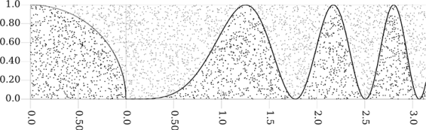
   This figure shows is associated with project 7. This shows how you can use picking random numbers to estimate the area under curves. This figure shows two curves and random points in square regions that bound those curves. The points that are below the curves are darker than those above. The fraction of points below is proportional to the area under the curve.

   $A\frac{N_{below}}{N_{total}},$

   where A is the area of the box. The more points you draw randomly, the more accurate the estimate.

   Write a recursive function with the following signature.

   def countUnder(nPnts:Int,xmin:Double, xmax:Double, ymin:Double,

    ymax:Double,f: Double=>Double):Int

   This function should generate the specified number of random points in the rectangle with the given bounds and return how many of them were below the curve defined by the function f. Note that you can get a random number in the range [min, max) with code like this.

   val r = min+math.random()*(max-min)

   You want to do this for the x and y axes.

   To estimate π use a function of $\sqrt{1-x^2}$ with x and y in the range of [0, 1). The full rectangle has an area of 1 while the area under the curve is π/4. If you multiply the fraction of points under the curve by 4, you get an estimate of pi.3

   In addition to printing out your estimate of π, you should print out an estimate of

   ${\displaystyle \underset{0}{\overset{\pi }{\int }}{(\sin x^2)}^2}$

   for the same number of random points.

8. If you did project 1 (p.108), you can now add another option to it. Write a function that takes a rational number as an (Int,Int) and returns an (Int,Int) where all common factors have been removed so that it is in the lowest form.

   With that added in, write a script that uses a recursive function to do calculations on rational numbers. The script presents the user with a menu with options for add, subtract, multiply, divide, and quit. If one of the first four options is selected, it should ask for a fraction and perform that operation between the “current” fraction and the one entered. When the program starts, the “current” value will be $\frac{1}{1}$ represented by (1,1). After each operation you print the new current value, making sure it is always in the lowest form.

   The website provides additional exercises and projects with data files that you can process using input redirection.

1In the first half of this book, we generally assume that user input will be valid. Dealing with invalid input requires exception handling, which is discussed in chapter 22.

2Indeed, the term “smell” is the actual terminology used in the field of refactoring for things in code that are not quite right and should probably be fixed.