
Spatial Trees
A lot of the data that you deal with in certain fields of computing is spatial. There are certain data structures that you can use to make the process of finding elements in certain parts of space more efficient. These spatial data structures can increase the speed of certain operations dramatically, especially when there are large numbers of elements involved. This chapter will consider a few of the many options for doing this.
31.1 Spatial Data and Grids
Examples of spatial data can be bodies in a physics simulation or characters spread out across a large world in a game. The way these bodies or agents behave is generally influenced by the other things that are near them. This makes the problem of finding nearby neighbors an important one. To illustrate the nature of this problem, let us consider a simplified example. You are given N points in some M dimensional space. For visualization purposes, we will typically treat M = 2, but it could be higher. We want to find all pairs of points (p1, p2) such that the distance between them is less than a given threshold, |p2− p1| < T .
The easiest-to-write solution to this problem is a brute force approach that runs through all particles in one loop, with a nested loop that runs through all the particles after that one in the sequence and calculates and compares distances. If we model the points as anything that can be converted to Int => Double we can write a class that serves as the interface for all the approaches to basic neighbor visits that we will write.1
package scalabook.adt

abstract class NeighborVisitor[A <% Int => Double](val dim:Int) {

  def visitAllNeighbors(tDist:Double, visit:(A,A) => Unit)

  def visitNeighbors(i:Int, tDist:Double, visit:(A,A) => Unit)

  var distCalcs = 0

  def dist[A <% Int => Double](p1:A, p2:A):Double = {

    distCalcs += 1

    math.sqrt((0 until dim).foldLeft(0.0)((d,i) => {

    val di = p1(i)-p2(i)

    d+di∗di

   }))

  }

}
This class has a dist method as all of its subtypes will need to perform this calculation. It also takes an argument for the dimensionality of the space the points should be considered for. There are two methods defined here. One of them does a complete search across all the pairs of particles. The other does a search relative to just one point. The member named distCalcs is there simply for the purposes of benchmarking our different methods to see how many times they have to calculate the distance between points.
The brute force implementation of this looks like the following.
package scalabook.adt
class BruteForceNeighborVisitor[A <% Int => Double](
d:Int,
val p:IndexedSeq[A]
) extends NeighborVisitor[A](d) {
def visitAllNeighbors(tDist:Double, visit:(A,A) => Unit) {
for{i <- 0 until p.length
val pi = p(i)
j <- i+1 until p.length
val pj = p(j)
if dist(pi,pj)<=tDist} visit(pi,pj)
}
def visitNeighbors(i:Int, tDist:Double, visit:(A,A) => Unit) {
val pi = p(i)
for{j <- 0 until p.length
val pj = p(j)
if dist(pi,pj)<=tDist} visit(pi,pj)
}
}
The method for finding all pairs has an outer loop using the variable i that goes through all the indices. Inside that it runs through all the points after the current point in the sequence. This way it does not deal with the same pair of particles, in opposite order, twice. The creation of the variables pi and pj where they are in the code is intended to prevent unnecessary indexing into the IndexedSeq p.
While this code is easy to write it if fairly easy to see that the number of calls to dist scales as O(N2). This is acceptable for smaller values of N, but it makes the approach infeasible when N gets large.2 For that reason, we need to use alternate approaches that allow neighbors to be found with less effort than running through all of the other particles.
The simplest approach to doing this is a regular spatial grid. Using this approach, you break the space that the particles are in down into a grid of regularly spaced boxes of the appropriate dimension. For each box in the grid, we keep a list of the particles that fall inside of it. Searching for neighbors then requires only searching against particles that are on lists in cells that are sufficiently nearby. Here is code for an implementation of NeighborVisitor which uses this method.
package scalabook.adt
import collection.mutable
class RegularGridNeighborVisitor[A <% Int => Double](
val p:IndexedSeq[A]
) extends NeighborVisitor[A](2) {
private val grid = mutable.ArrayBuffer.fill(1,1)(mutable.Buffer[Int]())
private var currentSpacing = 0.0
private var min = (0 until dim).map(i => p.foldLeft(1e100)((d,p) => d min p(i)))
private var max = (0 until dim).map(i => p.foldLeft(-1e100)((d,p) => d max p(i)))
def visitAllNeighbors(tDist:Double, visit:(A,A) => Unit) {
if(tDist<0.5∗currentSpacing || tDist>5∗currentSpacing) rebuildGrid(tDist)
val mult = math.ceil(tDist/currentSpacing).toInt
val offsets = Array.tabulate(2∗mult+1,2∗mult+1)((i,j) => (i-mult,j-mult)).
flatMap(i => i).filter(t => t._2>0 || t._2==0 && t._1>=0)
for{cx <- grid.indices
cy <- grid(cx).indices
(dx,dy) <- offsets
val gx = cx+dx
val gy = cy+dy
if gx>=0 && gx<grid.length && gy>=0 && gy<grid(gx).length
i <- grid(cx)(cy).indices
val pi = p(grid(cx)(cy)(i))} {
if(dx==0 && dy==0) {
for{j <- i+1 until grid(cx)(cy).length
val pj = p(grid(cx)(cy)(j))
if dist(pi,pj)<=tDist} visit(pi,pj)
} else {
for{j <- grid(gx)(gy)
val pj = p(j)
if dist(pi,pj)<=tDist} visit(pi,pj)
}
}
}
def visitNeighbors(i:Int, tDist:Double, visit:(A,A) => Unit) {
if(tDist<0.5∗currentSpacing || tDist>5∗currentSpacing) rebuildGrid(tDist)
val mult = math.ceil(tDist/currentSpacing).toInt
val offsets = Array.tabulate(2∗mult+1,2∗mult+1)((i,j) => (i-mult,j-mult)).
flatMap(i => i)
val cx = ((p(i)(0)-min(0))/currentSpacing).toInt
val cy = ((p(i)(1)-min(1))/currentSpacing).toInt
val pi = p(i)
for{(dx,dy) <- offsets
val gx = cx+dx
val gy = cy+dy
if gx>=0 && gx<grid.length && gy>=0 && gy<grid(gx).length
j <- grid(gx)(gy)
if i!=j
val pj = p(j)
if dist(pi,pj)<=tDist} visit(pi,pj)
}
/∗∗
∗ Rebuild the grid to a size that is appropriate for the searches. Note that
∗ this method was not written for efficiency. A true implementation should
∗ include a rewrite of this method.
∗/
def rebuildGrid(spacing:Double) {
min = (0 until dim).map(i => p.foldLeft(1e100)((d,p) => d min p(i)))
max = (0 until dim).map(i => p.foldLeft(-1e100)((d,p) => d max p(i)))
val cells = (0 until dim).map(i => ((max(i)-min(i))/spacing).toInt+1)
if(grid.size<cells(0)) grid.append(mutable.Buffer.fill(cells(0)-grid.size)
(mutable.ArrayBuffer.fill(cells(1)) (mutable.Buffer[Int]())):_∗)
else if(grid.size>cells(0)) grid.trimEnd(grid.size-cells(0))
for(col <- grid) {
if(col.size<cells(1))
col.append(mutable.Buffer.fill(cells(1)-col.size)(mutable.Buffer[Int]()):_∗)
else if(col.size>cells(1)) col.trimEnd(col.size-cells(1))
col.foreach(_.clear)
}
for(i <- p.indices) {
val cx = ((p(i)(0)-min(0))/spacing).toInt
val cy = ((p(i)(1)-min(1))/spacing).toInt
grid(cx)(cy) += i
}
currentSpacing = spacing
}
}
Clearly this code is longer and more complex than the brute force approach. However, there are many situations for which this will produce O(N) behavior for the method that visits all neighbor pairs and O(1) behavior for only the neighbors of a single particle.
This grid is hard coded to support only two dimensions. While not impossible, it is significantly more challenging to write code that uses arrays of arbitrary dimensions. Beside that point, regular grids do not work well in high dimensions. Imagine you have a n-dimensional cube and your search radius is about 1/100th the size of the cell so you want 100 divisions in each dimension. For a 2-D space this gives a modest 10, 000 = 104 cells in the grid. For a 3-D space you get a cube with 1, 000, 000 = 106 cells. As the dimensions go up, this continues to grow as 102n. This causes significant problems above three dimensions, especially as most problems will need more than 100 bins per dimension. We could write a 3-D grid, but there really are not many applications where it helps to go above that.
The situations when a grid approach is ideal are those where the particles are fairly uniformly distributed, the search radius is small compared to the whole area, and the area increases with N, not the density. In other words, if the number of neighbors for every particle is fairly similar and when N is increased, the points are added in such a way that the number of neighbors stays the same, then the grid is pretty much an optimal structure. To give an idea of how good the grid is, a simple run was done with 1000 points spread randomly and uniformly across a square region, an ideal configuration for a grid. The brute force approach always does N ∗ (N −1)/2 = 499500 distance calculations. The number for the grid varies with the random distribution of the particles and the search size. However,using a search distance 1/100th the size of the point distribution was never seen to need more than 500 distance comparisons to find between 100 and 200 neighbor pairs.
It is also important to note that building the grid is an O(N) operation. So assuming that the input for the program you are working on fits the conditions listed above, you can build a grid and find all the neighbors for all the particles in O(N) operations. That is a dramatic improvement over the O(N2) behavior of the brute force approach. The brute force approach starts to become intractable around 106 particles and even before that it is slow on most machines for N= 105. With the grid approach, speed is likely not the limiting factor. However many points you can deal with in the memory of the machine, you can probably process them as well.
31.2 Quadtrees and Octrees
What about situations for which the grid is not well suited? The most obvious example is when the points are not well distributed. Consider the distribution of points shown in figure 31.1. Here there are two regions of very high-density surrounded by reduced density around that. The sample grid drawn on the region would work fairly well for the low-density regions as each cells has only a few points in it. However, the grid is not helping much in the high-density regions. The grid based search would still be running through a very large number of particle pairs. However, if the grid were drawn with a size appropriate for the high-density regions, the low-density regions would be mostly empty cells and lots of time could be wasted processing them. It is even possible that the memory overhead of keeping all those empty cells could be a problem.
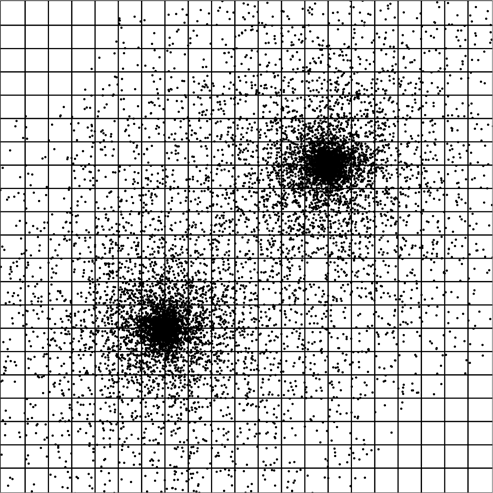
This figure shows an example set of points with a very non-uniform spatial distribution. A regular grid is laid over this to make clear how the point density in the grid cells will vary dramatically. The grid size shown here works well for many of the low-density regions where there are only a handful of particles per cell. A grid that only had a few particles per cell in the high-density regions would be a very fine grid with an extremely large fraction of the cells being empty in the low-density areas.
The way around this is to use a tree. Just like the Binary Search Tree (BST) is a more dynamic and adjustable structure than a sorted array, spatial trees have the ability to adjust resolution to the nature of the data in different areas. In some ways, you could picture a BST tree as a spatial tree in a 1-D space. There is a complete ordering of value along a given line. Some thought has to be given to how this can be extended to deal with systems where there are multiple, orthogonal orderings. Many different approaches to this have been developed, we will consider two of them explicitly in this chapter.
The easiest spatial tree to understand is probably the quadtree. There are multiple types of quadtree. We will focus on a region-based quadtree. For this tree, each node represents a square region of space. We start with a bounding square that contains all of the points we are dealing with. That region is represented by the root of the tree. Each node can have four children. The children each represent the equally sized quadrants of of their parent. With this tree the points all go into the leaves. How many points are allowed in each leaf varies with the application. Empirical testing can be used to find what works best. When there are more points in a region than is allowed, that region splits into the four children and the points are moved down.3
The results of building a quadtree with some non-uniform data is shown in figure 31.2. This tree has roughly 1000 data points in it. You can see that in regions where there are few points, the divisions are large. However, in the higher density sections of the tree, the cells divide down to very small sizes to isolate the points.
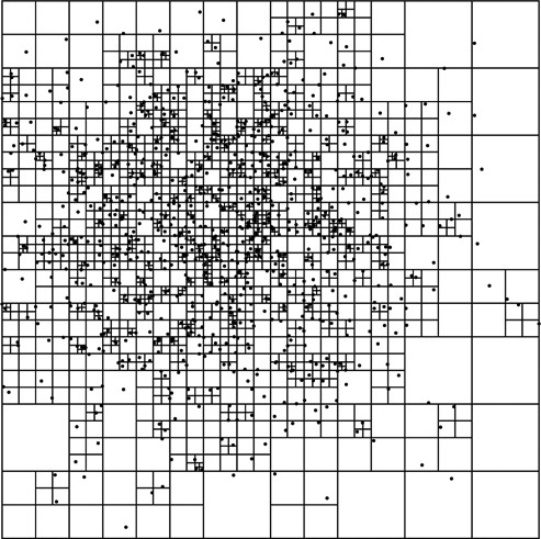
This is a quadtree with a number of non-uniformly distributed points to illustrate how the space is partitioned. For this example, each node is only allowed to hold a single point. The key advantage of the tree-based approach is that the resolution does not have to be uniform. Higher-density regions can divide the space much more finely.
The code for this tree is shown below. Like the grid, the quadtree is used for a 2-D spacial division and that is hard written into the code. The tree has a supertype called Node with two subtypes called LNode and INode for leaf node and internal node, respectively. The way this code is set up, only the leaf nodes hold particles. For this reason, it makes sense to use the approach of having two subtypes as they store very different data other than the location information. The INode also has additional functionality for splitting particles across the children and building the lower parts of the tree. The method childNum returns a number between 0 and 3 that is the index for a child based on location. The groupBy collection method is called as an easy way to get the different particles in each quadrant.
package scalabook.adt
class QuadtreeNeighborVisitor[A <% Int => Double](
val p:IndexedSeq[A]
) extends NeighborVisitor[A](2) {
private class Node(val cx:Double, val cy:Double, val size:Double)
private class LNode(x:Double, y:Double, s:Double, val pnts:IndexedSeq[Int])
extends Node(x,y,s)
private class INode(x:Double, y:Double, s:Double, pnts:IndexedSeq[Int]) extends
Node(x,y,s) {
val children = {
val groups = pnts.groupBy(pn => childNum(p(pn)(0),p(pn)(1)))
val hs = s∗0.5
val qs = s∗0.25
val ox = cx-qs
val oy = cy-qs
Array.tabulate(4)(i => makeChild(ox+hs∗(i%2),oy+hs∗(i/2), hs,
if(groups.contains(i)) groups(i) else IndexedSeq[Int]()))
}
def makeChild(x:Double, y:Double, s:Double, pnts:IndexedSeq[Int]):Node =
if(pnts.length>maxPoints) new INode(x,y,s,pnts)
else new LNode(x,y,s,pnts)
def childNum(x:Double, y:Double):Int = (if(x>cx) 1 else 0)+(if(y>cy) 2 else 0)
}
private val maxPoints = 1
private val root = {
val minx = p.foldLeft(1e100)((mx,pnt) => pnt(0) min mx)
val maxx = p.foldLeft(-1e100)((mx,pnt) => pnt(0) max mx)
val miny = p.foldLeft(1e100)((my,pnt) => pnt(1) min my)
val maxy = p.foldLeft(-1e100)((my,pnt) => pnt(1) max my)
val cx = 0.5∗(minx+maxx)
val cy = 0.5∗(miny+maxy)
val s = (maxx-minx) max (maxy-miny)
if(p.length>maxPoints) new INode(cx,cy,s,p.indices)
else new LNode(cx,cy,s,p.indices)
}
def visitAllNeighbors(tDist:Double, visit:(A,A) => Unit) {
for(i <- 0 until p.length) {
val pi = p(i)
def recur(n:Node):Unit = n match {
case ln:LNode =>
ln.pnts.filter(j => j>i && dist(pi,p(j))<=tDist).foreach(j => visit(pi,p(j)))
case in:INode =>
val x = pi(0)
val y = pi(1)
if(x+tDist>in.cx) {
if(y+tDist>in.cy) recur(in.children(3))
if(y-tDist<=in.cy) recur(in.children(1))
}
if(x-tDist<=in.cx) {
if(y+tDist>in.cy) recur(in.children(2))
if(y-tDist<=in.cy) recur(in.children(0))
}
}
recur(root)
}
}
def visitNeighbors(i:Int, tDist:Double, visit:(A,A) => Unit) {
val pi = p(i)
def recur(n:Node):Unit = n match {
case ln:LNode =>
ln.pnts.filter(j => j!=i && dist(pi,p(j))<=tDist).foreach(j =>
visit(pi,p(j)))
case in:INode =>
val x = pi(0)
val y = pi(1)
if(x+tDist>in.cx) {
if(y+tDist>in.cy) recur(in.children(3))
if(y-tDist<=in.cy) recur(in.children(1))
}
if(x-tDist<=in.cx) {
if(y+tDist>in.cy) recur(in.children(0))
if(y-tDist<=in.cy) recur(in.children(2))
}
}
recur(root)
}
}
The construction of the tree itself happens in the declaration of root. The type of quadtree must have a bounds containing the points so that is calculated first. After that is done, the proper node to is instantiated. that node serves as the root, and if it is an INode, it builds the rest of the tree below it. While this tree does not take advantage of it, one of the big benefits of the region-based quadtree is that it is fairly easy to write a mutable version that allows the user to add points one at a time as long as the user specifies an original bounding region.
The visitAllNeighbors and visitNeighbors methods include nested recursive functions that run through the tree looking for neighbors. The behavior on an INode is such that recursive calls are only made on children that the search area actually touches. When run on the same type of uniform random configuration used for the grid above, this tree did a bit fewer than twice as many distance calculations as the grid. This was still vastly better than the brute force approach and remarkably close to the grid considering the configuration of points used was ideal for the grid.4
As with the grid, the quadtree is inherently 2-D. A 3-D version that divides each node into octants is called an octree. We will build one of those in a later section. Also like the grid, this type of tree does not scale well to higher dimensions. This is due to the fact that the number of children contained in each child node scales as 2n for an n dimensional space. Given that the number of internal nodes scales as the number of points, having large internal nodes that store many children becomes inefficient. There are alternate ways of storing children, but if you really need a high-dimensional space, the next tree we will discuss is your better bet.
Before leaving the topic of the quadtree, it is also worth noting that this region-based quadtree is inherently unbalanced. The depth of the tree is significantly larger in regions of high-density. In practice, this does not introduce significant inefficiency, but it it worth noting as it is a real different from the BST tree.
31.3 kD-Trees
What should you do if you have to deal with a high-dimensional space, want a balanced spatial tree, and/or have dramatically different sizes in different dimensions that you want to resolve as needed? A possible solution to all of these is the use of a kD-tree. The "kD" in the name means k-dimensional so the name itself points to the fact that this tree is intended to scale to higher dimensions.
The way that a kD-tree works is that internal nodes have two children split across a plane that is perpendicular to one axis. Put more simply, you pick a dimension and a value, anything less than or equal to the value in that dimension goes to the left and anything greater than it goes to the right. This behavior should be fairly easy to understand as it is remarkably similar to a BST tree.
How you pick the dimension and the split value can vary greatly between applications. We will use a technique that tries to maximize the efficiency of each split and guarantees the tree is balanced. The split dimension will be the dimension with the largest spread. To pick a value, we will use the median value in that dimension. That way, the number of points on the left and the right will be as close to equal as possible, resulting in a balanced tree. Figure 31.3 shows a 2-D tree generated using this approach allowing three points per leaf. The fact that there is no bounding box here is intentional. The kD-tree puts in divisions that span as far as needed. The ones at the ends are effectively infinite. The internal ones are cut off by other splits.
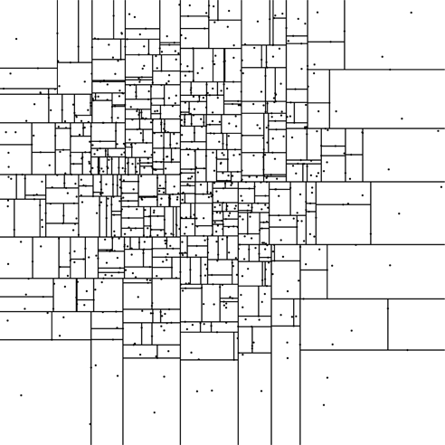
This is a kD-tree with a number of non-uniformly distributed points to illustrate how the space is partitioned. For this example, each node can hold up to three points. While this example only uses two dimensions, it is simple to scale the kD-tree up higher without adding overhead.
A sample code implementing NeighborVisitor using a kD-tree is shown here. This class is not hard coded to a specific dimensionality as there is nothing that ties it to a particular number of dimensions. There are many similarities between this code and the quadtree code so we will focus on differences. The first is that the IndexedSeq that is passed in is converted to a private Array. This forces the additional requirement of a manifest, but it greatly improves the efficiency of building the tree.
package scalabook.adt
class KDTreeNeighborVisitor[A <% Int => Double : Manifest](
d:Int,
val pIn:IndexedSeq[A]
) extends NeighborVisitor[A](d) {
private val p = pIn.toArray
private val maxPoints = 3
class Node
private class LNode(val pnts:Seq[Int]) extends Node
private class INode(start:Int, end:Int) extends Node {
val splitDim = {
val min = (0 until dim).map(i => p.view.slice(start,end).
foldLeft(1e100)((m,v) => m min v(i)))
val max = (0 until dim).map(i => p.view.slice(start,end).
foldLeft(-1e100)((m,v) => m max v(i)))
(0 until dim).reduceLeft((i,j) => if(max(j)-min(j)>max(i)-min(i)) j else i)
}
val (splitVal,left,right) = {
val mid = start+(end-start)/2
indexPartition(mid,start,end)
(p(mid)(splitDim),makeChild(start,mid+1),makeChild(mid+1,end))
}
def indexPartition(index:Int, start:Int, end:Int) {
if(end-start>1) {
val pivot = if(end-start<3) start else {
val mid = start+(end-start)/2
val ps = p(start)(splitDim)
val pm = p(mid)(splitDim)
val pe = p(end-1)(splitDim)
if(ps<=pm && ps>=pe || ps>=pm && ps<=pe) start
else if(ps<=pm && pm<=pe || ps>=pm && pm>=pe) mid else end-1
}
val ptmp = p(pivot)
p(pivot) = p(start)
p(start) = ptmp
var (low,high) = (start+1,end-1)
while(low<=high) {
if(p(low)(splitDim)<=ptmp(splitDim)) {
low += 1
} else {
val tmp = p(low)
p(low) = p(high)
p(high) = tmp
high -= 1
}
}
p(start) = p(high)
p(high) = ptmp
if(high<index) indexPartition(index,high+1,end)
else if(high>index) indexPartition(index,start,high)
}
}
def makeChild(s:Int, e:Int):Node = {
if(e-s>maxPoints) new INode(s,e) else new LNode(s until e)
}
}
private val root = new INode(0,p.length)
def visitAllNeighbors(tDist:Double, visit:(A,A) => Unit) {
for(i <- 0 until p.length) {
val pi = p(i)
def recur(n:Node):Unit = n match {
case ln:LNode =>
ln.pnts.foreach(j => if(j>i && dist(p(j),pi)<=tDist) visit(pi,p(j)))
case in:INode =>
if(pi(in.splitDim)-tDist<=in.splitVal) recur(in.left)
if(pi(in.splitDim)+tDist>in.splitVal) recur(in.right)
}
recur(root)
}
}
def visitNeighbors(i:Int, tDist:Double, visit:(A,A) => Unit) {
val pi = p(i)
def recur(n:Node):Unit = n match {
case ln:LNode =>
ln.pnts.foreach(j => if(j!=i && dist(p(j),pi)<=tDist) visit(pi,p(j)))
case in:INode =>
if(pi(in.splitDim)-tDist<=in.splitVal) recur(in.left)
if(pi(in.splitDim)+tDist>in.splitVal) recur(in.right)
}
recur(root)
}
}
The real meat of this code is in the creation of an INode. All that is passed in is a start and an end index into the array to represent what points are supposed to be under this node. All manipulations are done in place reordering elements in the array p.
The first thing done upon construction of an INode is to find the dimension in which the specified points have the largest spread to make it the split dimension. After this is the declaration and assignment to splitVal, left, and right. Most of the work done here occurs in the method indexPartition. The purpose of this method is to arrange the elements of the array along the split dimension such that the point which should be at index is located there and all the points below or above it along the appropriate dimension are above or below it in the array. In this case we happen to always be finding the median, but the code itself is more general than that. This function can find the element at any given index and do so in O(N) time.
The way this is done is that the function works very much like a quicksort. The base case is a single element. If there are more elements, a pivot it selected and that pivot is moved into place just like with would be in a quicksort. Where this differs it that it only recurses at most once. If the desired index is below the pivot, it recurses on the lower part. If it is above the pivot, the method recurses on the upper part. If the pivot happens to be at the desired index, the method returns. To see how this approach gives O(N) performance, simply recall that . As long as the pivot is always close to the center, this is roughly the way the amount of work behaves with each call.
It is interesting to note that because the elements in the p array are actually reordered, the LNode sequences of particle indices are always contiguous ranges. The visit methods are fairly straightforward. They are actually a fair bit simpler than their counterparts in the quadtree because there are only two children and a single split.
Running this code through the same 2-D tests that were done for the grid results in about four times as many distance calculations as we had for the quadtree. This is in part due to the fact that the leaves have three points in them. It is also somewhat due to the fact that nodes in the kD-tree can be elongated, even when the overall distribution of points is not. This is still far fewer distance calculations than the brute force approach and you would have to do empirical tests to determine which option was truly best for your application.
Another issue that impacts both the quadtree and the kD-tree is the problem of identical points. The quadtree will run into problems if you have any cluster of points with more than maxPoints with a spacing that is extremely small. Such a cluster will lead to very deep leaves as the nodes have to split repeatedly to resolve those points. The kD-tree does not suffer from tight clusters in the same way, but both will crash as there are more than maxPoints that all have the same location. The fact that those points can not be split, regardless of how far down the tree goes means that the code will try to create an infinite number of INodes to break them apart. The quadtree will run into this same problem if points are placed outside bounds, particular outside the corners.
31.4 Efficient Bouncing Balls
One example of an application where spatial data structures can be extremely beneficial is the bouncing balls problem that we made a Drawable for previously. For the 20-ball simulation that was performed previously, any spatial data structure is overkill. However, if the number of balls were increased by several orders of magnitude, a spatial data structure would become required.
If we were using a spatial data structure, the question of search radius arises. A single search radius that is safe for all particles is twice the maximum speed multiplied by the time step plus twice the maximum particle radius. As these values can be easily calculated in O(N) time, it is not a problem to add them to the code. It would be slightly more efficient to use a unique search radius for each particle that uses the speed and size of that particle plus the maximum values to account for the worst possibility for the other particle.
There are few changes that need to be made in the code for using a spatial data structure. You can find the original code in chapter 26 on page 687. Anyplace there is a call to findEventsFor, there is a need for the spatial data structure. The findEventsFor method takes a Seq[Int] with the indices of the particles that are to be searched against. The current implementation is brute force. It passes all indices after the current one in the timer when doing the complete search to initialize the queue and then all values other than the two involved in the collision for searching after a collision. The first one should use visitAllNeighbors with a visitor that calls the collisionTime method to see if the particles collide and adds them to the priority queue as needed. The call to findEventsFor is still needed to get wall collisions though it can be called with an empty list of other particles to check against as the call to visitAllNeighbors will have done that. The search for a single particle should use visitNeighbors to find the against list.
It is interesting to note the involvement of the timestep in the search radius. The code for the bouncing balls uses a time of 1.0 as the length of the timestep. This occurs in findEventsFor where there is a cutoff on the time for events to be added to the queue. If this were shortened, the particles would move less between frames being drawn. For the old method, there is not a significant motivation to do this other than to have the gravity integration be more accurate. For the spatial data structures, it can dramatically speed up the processing of finding collision events as it reduces the area that has to be searched.
31.5 End of Chapter Material
31.5.1 Summary of Concepts
- Spatial data comes in many forms and is associated with many areas of computing.
- Brute force techniques for doing things like finding nearby points in space tend to scale as O(N2).
- Spatial data structures can improve the scaling dramatically.
- Grids are simple and for low dimension, fairly uniform data, they are ideal.
- Region-based quadtrees and octrees divide a region that encompasses all the data into successively smaller, uniformly sized parts. This provides variable resolution for the places where it is needed.
- The kD-tree scales to arbitrarily high dimensions. Each internal node splits the data at a particular value with lower values going to the left and higher values to the right.
31.5.2 Exercises
- Write unit tests for the different spatial data structures that were presented in the chapter.
- Write a quadtree that includes an addPoint method.
- Parallelize any of the trees were presented in this chapter so that searches happen across multiple threads. If you want a bit more challenge, make it so that construction the the tree also occurs in parallel.
- Pick a spatial tree of your choosing and do speed tests on it. One way you can do this is to put random points in the tree and then search for all pairs below a certain distance. For each tree that was described, you can vary the number of points that are allowed in a leaf node. Do speed testing with different numbers of points in the data set as well as different numbers of points allowed in leaves.
It is also interesting to compare the relative speed of different trees of the same dimension.
31.5.3 Projects
- Pretty much any data can be viewed as existing in a space of the appropriate dimensions. If you ware working on the web spider, you should do exactly that to find things that are closely related in some way. What you do this on might depend on what data you are collecting. An obvious example would be if you were skimming box scores to a sport, you could make a space that has a different dimension for each significant statistical category. You could put all the entries you have in a kD-tree of that many dimensions, then do searches for everything within a certain distance of a particular point. This could show you things like players or teams that are comparable to one another in different ways.
If the data you are storing is not numerical, it is still possible to assign spatial values based on text or other information. For example, you could select a set of words that are relevant for what you are looking at and use a function of the number of times each word appears as a value for a different axis. If you have 100 different words of interest, this would mean you have a 100-D space that the pages would go into.5 These can be put into the kD-tree and that can be used to find pages that are similar according to different metrics.
Even if you are cataloging images, you can associate a sequence of numeric values with images. The numeric values could relate to factors like size, color, brightness, saturation, contrast, or many other things. The image is made of a lot of RGB values so there are many functions you could devise that produce something interesting.
- The MUD project is probably the one that has the least obvious use for spatial trees. After all, the maps in a MUD are completely text based, not spatial. Despite this, you can use an approach similar to what is described above for the web spider with the MUD as well. Characters, including player controlled and non-player controlled, likely have stats that indicate how powerful they are in different ways. These stats can be used to place them in a higher-dimensional space that you can map out with a kD-tree to enable functions like giving players the ability to find potential opponents or partners who are of similar capabilities.
It is also possible you might want to use a word count type of approach for a MUD, but this is likely to be less useful as you need many more data points than you have dimensions, and unless you have been very busy, the room count for your MUD is not likely to be all that high.
- Graphical games, both networked and not, have an automatic spatial nature to them. While your game might not really need a spatial data structure for locating things efficiently, you should put one in to give yourself experience with them. If you did create a game with a really big world, these spatial data structures could provide significant benefits.
- One interesting type of analysis that you could put into the math worksheet project is the ability to measure the fractal dimension of a set of data. There are many different formal definitions of fractal dimensions. We will use one called the correlation dimension. The correlation is determined using the correlation integral is formally defined as:
where g(ε) is the number of pairs of points with distance less than infinity. The correlation dimension can be found from using the relationship:
where ν is the correlation dimension and is equal to the slope of the correlation integral on a log-log plot. Finding this value requires two steps. First, we need to calculate C(ε). Once we have that, we need to take the log of both x and y values for all points on the curve and then do a linear fit to those points to find the slope.
Actually calculating C(ε) is O(N2) in the number of points, making it infeasible for a large data set. As the quality of the answer improves as N → ∞, it is better to have very large data sets and so a complete, brute force calculation becomes infeasible. That is where the spatial tree comes in. The number of points in nodes of different sizes provides an approximation of the number of pairs of points with a separation that length or shorter. To make this work, you need to use a tree where all the nodes at a particular level are the same size. This applies to our quadtree and octree constructions from the chapter. It can also apply to a kD-tree. The tree is constructed in a different way where splits are done down the middle spatially instead of at the median point. Once you have built such a tree, you can use the approximation that
This says that the number of pairs separated by ε or less goes as the sum over all cells of size ε of the number of cells in each cell squared. This technically over counts connections in a cell by a factor of two, but it does not count any connections between cells. In addition, any multiplicative error will be systematic across all levels so the value of ν will not be altered
Once you have a set of points representing C(ε), the last thing to do is to perform a linear fit to the points (log(ε), log(C(ε))). A linear least squares fit can be done by solving a linear equation much like what was done in project 6 (p.416). The idea is that you want to find optimal coefficients, ci, to minimize the sum of the squares of the following differences for your data points, (xj , yj) = (εj, C(εj)).
This can be done by solving the equation AT Ax = AT y, where
and y is the column vector of your yj values.
For a simple linear equation, there are only two terms so f1(x) = x and f2(x) = 1. That would reduce down to a 2x2 matrix that is fairly easy to solve. For this problem, you can typically reduce the problem even further by making the assumption that C(0) = 0. This is true as long as no two points every lie at exactly the same location. In that case, and . The value of the one coefficient can be found by simple division.
- If you have been working on the Photoshop® project, you can use a 2-D kD-tree to create an interesting filter for images. The kD-tree filter breaks the pixels in an image up into small regions and colors each leaf a single color. This can give something of a stained glass effect with rectangular regions. You can choose how to do the divisions to give the effect that you want. One recommendation is to make cuts in alternating dimensions such that you balance the brightness or the total intensity of a color channel on each side. So if the first cut is vertical, you find the location where the total amount of red to the left of the cut and the total to the right of the cut are as close as possible. Then you do horizontal cuts on each side of that following the same algorithm. After a specified number of cuts, you stop and average the total color of all pixels in each region. Use that average color to fill that region.
- Spatial trees can be used to improve collision handling in the simulation workbench. Project 6 (p.416) described how collision finding is O(n2) by default and looked at a way to improve that for most timesteps. Spatial data structures can also be used to reduce the number of pairs that have to be checked. The simplest approach just uses the tree to search for particles that are within a particular search radius of the particle in question. The search radius is given by ΔvΔt + 2Rmax, where Δv is the relative velocity of particles, Δt is the time step, and Rmax is radius of the largest particle. This should take the number of pairs checked down from O(n2) to O(n log(n)).
1This is written as a class instead of a trait to keep the code simpler. The <% symbol gets expanded out to include an implicit argument. As traits can not take arguments, we would have to get into the more complex details of this in order to use a trait. See appendix B for details.
2The author does large-scale simulations where N typically varies from 105 to more than 108. He once needed to check if a bug had caused any particles to be duplicated. As a first pass, he wrote a short piece of code like this to do the check. When it did not finish within an hour, the author took the time to do a little calculation of how long it would take. That particular simulation had a bit over 107 particles. The answer was measured in weeks. Needless to say, he took the time to implement one of the methods from this chapter instead.
3It is worth noting again that this is something of a standard implementation of a region based quadtree. Different aspects can be varied depending on the application. We will see an alternative approach later in this chapter for the closely related octree.
4The version of visitAllNeighbors shown here is very similar to putting visitAllNeighbors in a loop. This approach has one drawback that the recursion goes through the higher nodes many times, duplicating work. It is possible to write a function that recurses over two Node arguments that improves on this. It was not shown here because it is significantly more complex and difficult for the reader to understand.
5Using word counts for the value is typically not ideal because the length of a page can dramatically impact where it appears in your space. For that reason you often want to do something like take the log of the word count or the relative fraction of the number of instances of the words