
Chapter 35
Augmenting Trees
Chapter 29 covered the basics of trees and how to use a binary search tree (BST) to implement the map Abstract Data Type (ADT). This implementation gave us the possibility of O(log(n)) performance for all the operations on that ADT. Unfortunately, it also allowed the possibility of O(n) performance if the tree were built in a way that made it unbalanced. In this chapter we will see how we can fix that flaw by adding a bit more data to nodes and using the data to tell us when things are out of balance so that operations can be performed to fix the situation. In addition, we will see how we can use a similar approach to let us use a tree as the storage mechanism behind a sequence ADT implementation that is O(log(n)) for direct access, inserting, and removing.
35.1 Augmentation of Trees
The general idea of this chapter is that we are going to add some additional data into our tree nodes to give the tree additional capabilities. If you go back and look at the implementation of the BST, each node kept only a key, the data, the left child, and the right child. Augmenting data can deal with data values stored in subtrees or they can deal only with the structure of the tree itself.
There is one key rule for augmented data, it must be maintainable in O(log(n)) operations for any of the standard methods. If this is not the case, then the augmentation will become the slowest part of the tree and it will become the limiting factor in overall performance. Fortunately, any value that you can calculate for a parent based solely on the values in the children will have this characteristic assuming it does not change except when tree structure changes. You can be certain such a value is maintainable in O(log(n)) operations because operations like add and remove from a tree only touch O(log(n)) nodes as they go from the root down to a leaf. Maintaining the augmented values only requires updating nodes going back from the leaf up to the root.
Example values include tree properties like height and size. The height of a node is the maximum of the height of the two children plus one. The size is the sum of the sizes of the two children plus one. Any value where the value of the parent can be found using a binary operation like min, max, +, or ∗ or the children will generally work. Even more complex values that require more than one piece of information can be calculated. Consider the example of an average of value in a subtree. An average can not be calculated as the simple binary combination of two averages. However, the average is calculated as the quotient of two sums. The first sum is the sum of all the values you want to average. The second sum is how many there are. This is basically size, which we just described as being a sum over the children plus one. If you annotate nodes with both of those values, it is simple to produce the average for any subtree.
35.2 Balanced BSTs
The first example of any annotated tree that we will consider is a form of self-balancing BST called an AVL tree. Recall from chapter 29 that the primary shortcoming of BST was that is could become unbalanced and then exhibit O(n) performance. Whether the BST was balanced or not was completely dependent on the order in which keys were added and removed. This is something that is very hard to control. A self-balancing tree does a bit of extra work to ensure that the tree always remains properly balanced, regardless of the order of the operations that are performed on it. The AVL tree was the first such tree to be described and is fairly simple to understand. [10]
The idea behind an AVL tree is that we want the height of the two children of any given node to be within one of each other. So if one child has a height of 5, the other child has to have a height of 4, 5, or 6 to be acceptable. If it does not meet this condition, the tree has to be adjusted to bring it back into compliance. This requirement of children being within one of each other in height keeps the tree as close to balanced as possible. However, it is rather restrictive and leads to a fair bit of adjustments. For that reason, it is more common for libraries to use other self-balancing trees like a red-black tree.
The AVL tree works exactly like a normal BST for searches. It is only for operations that add or remove nodes that heights have to be recalculated and adjustments have to be made. As long at the AVL condition is maintained, we can be certain that all the standard methods will complete in O(log(n)) operations.
35.2.1 Rotations
The typical approach to re-balancing trees that have gotten unbalanced is through rotations. The idea of a rotation is to pull one of the children of a node up above the parent and swap on grandchild across to the other child in such a way that the proper BST ordering is preserved while pulling a grandchild that has grown too tall up to restore balance. The two basic rotations, to the right and the left are shown in figure 35.1. A single rotation to the right can be used when the outer left grandchild has gotten too tall so that the height of the left child is two greater than the right child. Conversely, a single left rotation can fix the problem when the outer right grandchild has gotten too tall. These types of imbalance can occur when an add operation adds a new child to a subtree that increases its total height.
Note that the subtrees A, B, and C in figure 35.1 are shown without any detail other than one of them is taller than the other two. This is intentional. We do not care about the internal structure of those subtrees, only their overall heights.
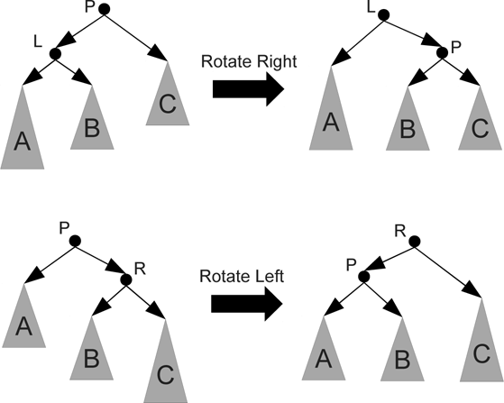
This figure shows single rotations to the left and the right. These rotations can be used when a node becomes unbalanced because the outer grandchild on the left or the right grows too tall.
In the situation where an internal grandchild, that is to say the right child of the left child or the left child of the right child, has grown to make the tree unbalanced two rotations are required. The first rotation is applied to the child that has the greater height, moving it outward. The second rotation then moves the parent to the opposite side. Figure 35.2 shows how this works. Note that each step in these double rotations is one of the single rotations shown in figure 35.1. This is significant in code as well because after the single rotations have been implemented, it is a simple task to use them to build a double rotation.
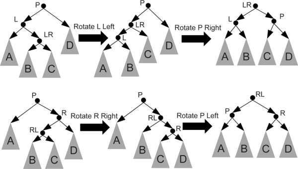
This figure shows double rotations to the left-right and the right-left. These rotations can be used when a node becomes unbalanced because the inner grandchild on the left or the right grows too tall. Note that each of this is simply two applications of the rotations from figure 35.1.
35.2.2 Implementation
To implement an AVL tree, we will use the immutable BST written in chapter 29 as a base and edit it appropriately. Making a mutable AVL tree is left as an exercise for the reader. Like that tree, we have a public type that represents a tree with no functionality. We also have two private classes that implement the public type. The top-level type has two additions for functionality, rotate and height, as well as one for debugging purposes, verifyBalance. The rotate method is supposed to check the balance and perform appropriate rotations if needed. The height member stores the height of the node. It is an abstract val so the subtypes have to provide a value. Code for this is shown here.
package scalabook.adt
abstract sealed class ImmutableAVLTreeMap[K <% Ordered[K],+V] extends Map[K,V] {
def +[B >: V](kv:(K,B)):ImmutableAVLTreeMap[K,B]
def -(k:K):ImmutableAVLTreeMap[K,V]
def rotate:ImmutableAVLTreeMap[K,V]
val height:Int
def verifyBalance:Boolean
}
private final class AVLNode[K <% Ordered[K],+V](private val key:K,
private val data:V, private val left:ImmutableAVLTreeMap[K,V],
private val right:ImmutableAVLTreeMap[K,V]) extends ImmutableAVLTreeMap[K,V] {
val height = (left.height max right.height)+1
def +[B >: V](kv:(K,B)) = {
val ret = if(kv._1 == key) new AVLNode(kv._1, kv._2, left,right)
else if(kv._1 < key) new AVLNode(key, data, left+kv, right)
else new AVLNode(key, data, left, right+kv)
ret.rotate
}
def -(k:K) = {
val ret = if(k == key) {
left match {
case _:AVLEmpty[K] => right
case i:AVLNode[K,V] => {
right match {
case _:AVLEmpty[K] => left
case _ => {
val (k, d, newLeft) = i.removeMax
new AVLNode(k, d, newLeft, right)
}
}
}
}
} else if(k < key) {
new AVLNode(key, data, left-k, right)
} else {
new AVLNode(key, data, left, right-k)
}
ret.rotate
}
def get(k:K):Option[V] = {
if(k==key) Some(data)
else if(k<key) left.get(k)
else right.get(k)
}
def iterator = new Iterator[(K,V)] {
val stack = new ListStack[AVLNode[K,V]]
pushRunLeft(AVLNode.this)
def hasNext:Boolean = !stack.isEmpty
def next:(K,V) = {
val n = stack.pop()
pushRunLeft(n.right)
n.key -> n.data
}
def pushRunLeft(n:ImmutableAVLTreeMap[K,V]) {
n match {
case e:AVLEmpty[K] =>
case i:AVLNode[K,V] =>
stack.push(i)
pushRunLeft(i.left)
}
}
}
def rotate:ImmutableAVLTreeMap[K,V] = {
if(left.height>right.height+1) {
left match {
case lNode:AVLNode[K,V] => // Always works because of height.
if(lNode.left.height>lNode.right.height) {
rotateRight
} else {
new AVLNode(key,data,lNode.rotateLeft,right).rotateRight
}
case _ => null // Can't happen.
}
} else if(right.height>left.height+1) {
right match {
case rNode:AVLNode[K,V] => // Always works because of height.
if(rNode.right.height>rNode.left.height) {
rotateLeft
} else {
new AVLNode(key,data,left,rNode.rotateRight).rotateLeft
}
case _ => null // Can't happen.
}
} else this
}
def verifyBalance:Boolean = {
left.verifyBalance && right.verifyBalance && (left.height-right.height).abs<2
}
private def removeMax:(K,V,ImmutableAVLTreeMap[K,V]) = {
right match {
case e:AVLEmpty[K] => (key, data, left)
case i:AVLNode[K,V] =>
val (k, d, r) = i.removeMax
(k, d, new AVLNode(key,data,left,r).rotate)
}
}
private def rotateLeft:AVLNode[K,V] = right match {
case rNode:AVLNode[K,V] =>
new AVLNode(rNode.key,rNode.data,new
AVLNode(key,data,left,rNode.left),rNode.right)
case _ => throw new IllegalArgumentException("Rotate left called on node with
empty right.")
}
private def rotateRight:AVLNode[K,V] = left match {
case lNode:AVLNode[K,V] =>
new AVLNode(lNode.key,lNode.data,lNode.left,new
AVLNode(key,data,lNode.right,right))
case _ => throw new IllegalArgumentException("Rotate right called on node with
empty left.")
}
}
private final class AVLEmpty[K <% Ordered[K]] extends
ImmutableAVLTreeMap[K,Nothing] {
def +[B](kv:(K,B)) = {
new AVLNode(kv._1, kv._2, this, this)
}
def -(k:K) = {
this
}
def get(k:K):Option[Nothing] = {
None
}
def iterator = new Iterator[(K,Nothing)] {
def hasNext = false
def next = null
}
def rotate:ImmutableAVLTreeMap[K,Nothing] = this
def verifyBalance:Boolean = true
val height:Int = 0
}
object ImmutableAVLTreeMap {
def apply[K <%
Ordered[K],V](data:(K,V)∗)(comp:(K,K)=>Int):ImmutableAVLTreeMap[K,V] = {
val empty = new AVLEmpty[K]()
val d = data.sortWith((a,b) => comp(a._1,b._1)<0)
def binaryAdd(start:Int,end:Int):ImmutableAVLTreeMap[K,V] = {
if(start<end) {
val mid = (start+end)/2
new AVLNode(d(mid)._1,d(mid)._2,binaryAdd(start,mid),binaryAdd(mid+1,end))
} else empty
}
binaryAdd(0,data.length)
}
}
The additions to the AVLEmpty type are simple. The height is always 0, the rotate returns this because it is always balanced, and given that the verifyBalance method always returns true.
The internal node type is slightly more complex. The height is set to the obvious value of (left.height max right.height)+1. The verifyBalance method checks the heights of the children and recursively calls itself on those children. The real meat of the change is in the rotate method. This method checks the height of the children and if they are out of balance it performs one or two rotations to return a node that has a balanced subtree. The rotations themselves are implemented in private methods called rotateLeft and rotateRight.
There are a number of matches done in the different rotate methods. This is due to the fact that they have to get hold of left and right grandchildren. This requires a match because the top-level type does not have left and right. This makes sense as they are not defined on AVLEmpty. The way the code is written, it should not be possible to those methods to be called with an AVLEmpty node. The rotation methods are written to throw exceptions should that happen.
The only other changes are the additions of calls to rotate in the + and - methods. These calls occur popping back up the stack so the entire tree is rebalanced every time. Testing for this class begins with test code from the original BST. To ensure that it is working, a tree must be built using + then checked with verifyBalance. The shortcut approach that is implemented in the companion object was created to always produce a perfectly balanced tree so using it does not actually test the rotation code.
35.3 Order-Statistic Trees: Trees as Sequences
The AVL tree used an augmentation of height to enable self-balancing. Augmenting by size can produce a tree that works as a sequence that is fairly efficient for both random access as well as random insertion and removal. By fairly efficient, we mean O(log(n)) because it will keep the height augmentation and be a balanced tree.
Both the BST and the AVL tree have been used to implement the map ADT. The type we are describing here is a sequence. This is significant because the map ADT needs a key value that has an ordering by which data can be accessed. In a sequence, things are accessed by an index, not a key. What is more, the index of an element can change if other items are inserted or removed before it. The key for a map has to be immutable. Using mutable keys is a great way to produce errors with a map. So how does this work, and what does the size augmentation have to do with it?
Assume a binary tree where we say that the index is the key. This is much like a sequence where you look up values by the index. Figure 35.3 shows what this might look like. Letters have been used as the data here. On the left there is a sequence with nine characters in it and a balanced tree that has the same nine characters with numeric annotations. The number before the letter is the size of the node. The number after it is the index. On the right the letter 't' has been inserted at index 5. Note how this changes the index values of all the letters which had indexes greater than or equal to 5.
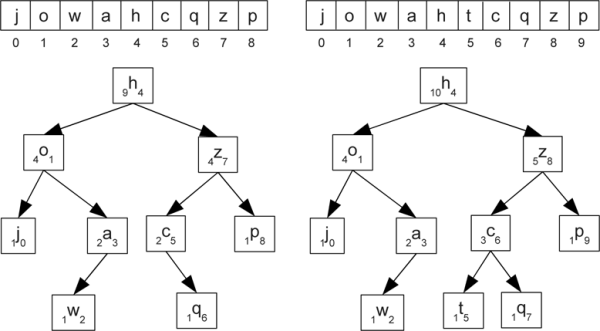
This figure shows two arrays and possible tree representations for them. The second was arrived at by adding the letter 't' at index 5 of the first. In the tree, each node has the value, a letter, drawn large with a preceding number that is the size of the node and a following number that is the index.
To use the tree as a sequence, we have to have an efficient way of finding nodes based on index. That would allow us to to direct access, as well as finding nodes or positions for inserting and removing. The key to associating index with nodes is in the size. The first indication of this is that the size of the node for 'o' is the same as the index of the root, 'h'. This is not coincidence. The size of 'o' is the number of nodes that are "before" the root in the sequence. Since indexes begin at 0, the index of the root should be the size of the left child. This logic holds throughout the tree so having the size allows us to do a binary search through an index.
To see this, assume that we want to find the item at index 6. We start by looking at the size of the left child. It is 4, which is less than 6. This tells us that what we are looking for is on the right side of the tree. This is the signature of a binary search. We do one comparison and it allows us to throw out half the data. So we go to the right child. We are not looking for index 6 on the right child though. Instead, we are looking for index 1. The left child was the first 4 and the root itself was another. So we have thrown out the first 5 elements and we subtract that from the index we are looking for.
So after one comparison we are on the subtree with 'z' at the top looking for index 1. The size of the left child is 2. This is larger than the index we are looking for, so we go to the left. When we move to the left, the index stays the same because we are not jumping past any elements. After two comparisons we are on 'c' looking for index 1. The left child of 'c' is empty and therefore has a size of zero. That is smaller than the index we are looking for so we go to the right and subtract 1 from the index we are looking for because we skipped the node with 'c'. We are now on the node with 'q' looking for index 0. The left child of 'q' is empty, giving it size zero, the same as the index we are looking for, and therefore 'q' is the value we are looking for.
This process illustrates how storing the size only can let us find values at indexes in a number of operations proportional to the height of the tree. That is slower than for an array, but significantly faster than what a linked-list would provide.
What would happen if we looked at index 6 again after adding the 't' ? Again, we start at 'h' and see the left child has size 4. Then we move to 'z' on the right looking for index 1. The left child has size 3 so we move to the left, still looking for index 1. The left child of 'c' has a size of 1 meaning that 'c' is the node we are looking for.
This same type of searching could be done with an index annotation. However, an index annotation can not be maintained efficiently. To see this, look closely at the differences between the numbers annotating the nodes in figure 35.3. The size values only changed for the nodes with 'c', 'z', and 'h'. That is the path from the new node up to the root, a path that will have length O(log(n)) in a balanced tree. The index annotation has changed for 'c', 'q', 'z', and 'p'. The is everything after the inserted value. In this case the difference is 3 to 4, but you can picture putting the new value at index 1 to see that the number of indexes that need to change scales as O(n). This tells us that we want to augment our nodes with size, not index values.
The code below is an implementation of an order-statistic tree that extends the mutable.Buffer trait. This class uses internals classes for Node and INode as well as an internal object declaration for Empty. While this mirrors some of the style of the immutable tree in the last section, this tree is mutable and everything in INode is a var. While this uses a similar class structure to the immutable AVL tree, it has a very different implementation with more overloaded methods and a lot fewer uses of match.
The code for the Buffer methods themselves are generally short, as are the methods in Empty. The majority of the code is in INode, specifically in the methods for removing and rotating. The use of Empty with methods for +, +:, and insert keep the insertion code short. The recurring theme we see in this code is comparing an index to the size of the left child.
package scalabook.adt
import collection.mutable
class OrderStatTreeBuffer[A] extends mutable.Buffer[A] {
abstract private class Node {
def size:Int
def height:Int
def +(elem:A):Node
def +:(elem:A):Node
def apply(n:Int):A
def remove(n:Int):(A,Node)
def removeMin:(A,Node)
def update(n:Int, elem:A):Unit
def insert(n:Int, elem:A):Node
def rotate:Node
}
private class INode(var data:A, var left:Node, var right:Node) extends Node {
var size = 1+left.size+right.size
var height = 1+(left.height max right.height)
private def setSizeAndHeight {
size = 1+left.size+right.size
height = 1+(left.height max right.height)
}
def +(elem:A):Node = {
right += elem
setSizeAndHeight
rotate
}
def +:(elem:A):Node = {
left += elem
setSizeAndHeight
rotate
}
def apply(n:Int):A = {
if(n==left.size) data
else if(n<left.size) left(n)
else right(n-left.size-1)
}
def remove(n:Int):(A,Node) = {
val ret = if(left.size==n) {
val d = data
if(right==Empty) (data,left)
else if(left==Empty) (data,right)
else {
val (newData,r) = right.removeMin
right = r
data = newData
setSizeAndHeight
(d,this)
}
} else if(left.size>n) {
val (d,l) = left.remove(n)
left = l
setSizeAndHeight
(d,this)
} else {
val (d,r) = right.remove(n-left.size-1)
right = r
setSizeAndHeight
(d,this)
}
(ret._1,ret._2.rotate)
}
def removeMin:(A,Node) = if(left==Empty) (data,right) else {
val (d,l) = left.removeMin
left = l
setSizeAndHeight
(d,rotate)
}
def update(n:Int, elem:A) {
if(n==left.size) data = elem
else if(n<left.size) left(n) = elem
else right(n-left.size-1) = elem
}
def insert(n:Int, elem:A):Node = {
if(n<=left.size) left = left.insert(n,elem)
else right = right.insert(n-left.size-1,elem)
setSizeAndHeight
rotate
}
def rotate:Node = {
if(left.height>right.height+1) {
left match {
case lNode:INode => // Always works because of height.
if(lNode.left.height>lNode.right.height) {
rotateRight
} else {
left = lNode.rotateLeft
rotateRight
}
case _ => null // Can't happen.
}
} else if(right.height>left.height+1) {
right match {
case rNode:INode => // Always works because of height.
if(rNode.right.height>rNode.left.height) {
rotateLeft
} else {
right = rNode.rotateRight
rotateLeft
}
case _ => null // Can't happen.
}
} else this
}
private def rotateLeft:INode = right match {
case rNode:INode =>
right = rNode.left
rNode.left = this
setSizeAndHeight
rNode.setSizeAndHeight
rNode
case _ => throw new
IllegalArgumentException("Rotate left called on node with empty right.")
}
private def rotateRight:INode = left match {
case lNode:INode =>
left = lNode.right
lNode.right = this
setSizeAndHeight
lNode.setSizeAndHeight
lNode
case _ => throw new
IllegalArgumentException("Rotate right called on node with empty left.")
}
}
private object Empty extends Node {
val size = 0
val height = 0
def +(elem:A):Node = new INode(elem,Empty,Empty)
def +:(elem:A):Node = new INode(elem,Empty,Empty)
def apply(n:Int):A = throw new
IllegalArgumentException("Called apply on Empty.")
def remove(n:Int):(A,Node) = throw new
IllegalArgumentException("Called remove on Empty.")
def removeMin:(A,Node) = throw new
IllegalArgumentException("Called removeMin on Empty.")
def update(n:Int, elem:A) = throw new
IllegalArgumentException("Called update on Empty.")
def insert(n:Int, elem:A):Node = new INode(elem,Empty,Empty)
def rotate:Node = this
}
private var root:Node = Empty
def +=(elem:A) = {
root = root+elem
this
}
def +=:(elem:A) = {
root = elem+:root
this
}
def apply(n:Int):A = {
if(n>=root.size) throw new
IndexOutOfBoundsException("Requested index "+n+" of "+root.size)
root(n)
}
def clear() {
root = Empty
}
def insertAll(n:Int, elems:Traversable[A]) {
var m = 0
for(e <- elems) {
root = root.insert(n+m,e)
m += 1
}
}
def iterator = new Iterator[A] {
var stack = mutable.Stack[INode]()
def pushRunLeft(n:Node):Unit = n match {
case in:INode =>
stack.push(in)
pushRunLeft(in.left)
case Empty =>
}
pushRunLeft(root)
def hasNext:Boolean = stack.nonEmpty
def next:A = {
val n = stack.pop
pushRunLeft(n.right)
n.data
}
}
def length:Int = root.size
def remove(n:Int):A = {
if(n>=root.size) throw new
IndexOutOfBoundsException("Remove index "+n+" of "+root.size)
val (ret,node) = root.remove(n)
root = node
ret
}
def update(n:Int, newelem:A) {
if(n>=root.size) throw new
IndexOutOfBoundsException("Update index "+n+" of "+root.size)
root(n) = newelem
}
}
Note that the rotations in this code look a bit different. This is because this code does mutating rotations where references are reset instead of building new nodes. That requires changing two references, them making sure that augmenting value are correct.
It is worth noting that the author wrote this code first without the rotations. It was a non-AVL binary tree that implemented the Buffer trait. That code was tested to make sure that it worked before it was refactored to do the AVL balancing. A non-AVL version of this data structure is likely to be little better than a linked list unless you happen to be doing a lot of random additions. With the rotations, the code behavior looks identical from the outside, but we can be certain of O(log(n)) performance for any single data element operation.1 The tree and rotations do add overhead though, so unless your collection needs to be quite large and you really need a lot of random access as well as random addition and deletion, this probably is not the ideal structure.
This data type is yet another example of why you need to know how to write your own data structures. The scala.collection.mutable package includes implementations of Buffer that are based on arrays and linked lists. It does not include an implementation based on an order-statistic tree. If your code needs the uniform O(log(n)) operations, you really need to be capable of writing it yourself.
35.4 Augmented Spatial Trees
Binary trees are not the only trees that can be augmented. There are very good reasons why you might want to augment spatial trees as well. The data you augment a spatial tree with is typically a bit different from that in a normal tree. For example, you might store average positions of points in a subtree or the total mass of particles in a subtree. In other situations, you want to know the extreme values in a tree for different directions. In the case of the collisions that we looked at in chapter 31, the tree nodes could store information on maximum velocity and radius in a subtree so that searches could be done using a search radius that adjusts to the properties of the local population. This can make things much faster in situations where one particle happens to be moving unusually fast or is significantly larger than the others.
To illustrate an augmented spatial tree, the final example in this book is going to be a bit different. We will create an octree that is intended to provide fast calculations for things like collisions or ray intersections. This tree will be different from our previous spatial trees in a few ways. Obviously, it will be augmented with some other data. We will use the minimum and maximum values in x, y, and z for the augmentation. In addition, objects that are added to the tree will be able to go in internal nodes, not just leaves. The augmentation is intended to give us an estimate of "when" a cell becomes relevant.2 The ability to store values high up in the tree is intended to let this structure work better for data sets where objects are of drastically different sizes. Something that is very large will have the ability to influence a lot more potential collisions or intersections than something very small. By placing objects at a height in the tree that relates to their size, we allow searches to "hit" them early and not have the bounds on lower levels of the tree altered by one large object. This is not the same as putting in a node that completely contains them. That would put any object, even small ones, that happen to fall near a boundary high up in the tree.
The code for such a tree is shown below. The class is called a IntersectionOctree. There is a companion object that defines two traits that need to be extended by any code wanting to use this structure. One has methods needed by object that are put in the tree and the other is a type that can be used to check for intersections based on different criteria. The type parameter on IntersectionOctree must inherit from the former. When an octree is built, the calling code needs to give it a sequence of objects, a center for the octree, a size for the octree, and a minimum size to split down to. This last parameter will prevent the tree from becoming extremely deep is a very small object is added.
package scalabook.adt
import collection.mutable
class IntersectionOctree[A <: IntersectionOctree.IntersectionObject](
objects:Seq[A], centerX:Double, centerY:Double, centerZ:Double,
treeSize:Double,minSize:Double) {
private class Node(val cx:Double,val cy:Double,val cz:Double,val size:Double) {
val objs = mutable.Buffer[A]()
var children:Array[Node] = null
var min:Array[Double] = null
var max:Array[Double] = null
import IntersectionOctree.ParamCalc
def add(obj:A) {
if(obj.size>size∗0.5 || size>minSize) objs += obj
else {
if(children==null) {
val hsize = size∗0.5
val qsize = size∗0.25
children = Array.tabulate(8)(i =>
new Node(cx-qsize+hsize∗(i%2), cy-qsize+hsize∗(i/2%2),
cz-qsize+hsize∗(i/4), hsize))
}
children(whichChild(obj)).add(obj)
}
}
private def whichChild(obj:A):Int = {
(if(obj(0)>cx) 1 else 0)+(if(obj(1)>cy) 2 else 0)+(if(obj(2)>cz) 4 else 0)
}
def finalizeNode {
if(children!=null) children.foreach(_.finalizeNode)
min = (0 to 2).map(i =>
objs.view.map(_.min(i)).min min
(if(children==null) 1e100 else children.view.map(_.min(i)).min)).toArray
max = (0 to 2).map(i =>
objs.view.map(_.max(i)).max max
(if(children==null) -1e100 else children.view.map(_.max(i)).max)).toArray
}
def findFirst(pc:ParamCalc[A]):Option[(A,Double)] = {
val o1 = firstObj(pc)
val o2 = firstChildObj(pc)
(o1,o2) match {
case (None,_) => o2
case (_,None) => o1
case (Some((_,p1)),Some((_,p2))) => if(p1<p2) o1 else o2
}
}
private def firstObj(pc:ParamCalc[A]):Option[(A,Double)] = {
objs.foldLeft(None:Option[(A,Double)])((opt,obj) => {
val param = pc(obj)
if(opt.nonEmpty && opt.get._2<param) opt else Some(obj,param)
})
}
private def firstChildObj(pc:ParamCalc[A]): Option[(A,Double)] = {
if(children==null) None else {
val cparams = for(c <- children; val p=pc(min,max); if
c!=Double.PositiveInfinity) yield c -> p
for(i <- 1 until cparams.length) {
val tmp = cparams(i)
var j = i-1
while(j>0 && cparams(j)._2>tmp._2) {
cparams(j+1) = cparams(j)
j -= 1
}
cparams(j+1) = tmp
}
var ret:Option[(A,Double)] = None
var i=0
while(i<cparams.length && (ret.isEmpty || cparams(i)._2>ret.get._2)) {</cparams.length>
val opt = cparams(i)._1.findFirst(pc)
if(opt.nonEmpty && (ret.isEmpty || opt.get._2<ret.get._2)) ret = opt
i += 1
}
ret
}
}
}
private val root = new Node(centerX,centerY,centerZ,treeSize)
objects.foreach(root.add)
root.finalizeNode
def findFirst(pc:IntersectionOctree.ParamCalc[A]):Option[(A,Double)] = {
root.findFirst(pc)
}
}
object IntersectionOctree {
trait IntersectionObject extends (Int => Double) {
def apply(dim:Int):Double
def min(dim:Int):Double
def max(dim:Int):Double
def size:Double
}
/∗∗
∗The A => Double should calculate the intersect parameter for an object.
∗The (Array[Double],Array[Double) => Double should calculate it for a box
∗with min and max values
∗/
trait ParamCalc[A <: IntersectionOctree.IntersectionObject] extends
(A => Double) with ((Array[Double],Array[Double])=>Double)
}
The way the tree is defined, it is mutable with an add method. However, before any tests can be done for intersections, the finalizeNode method has to be called on the tree. As it is written, all objects are added and the tree is finalized at the original construction.
The finalizeNode method has the task of setting the minimum and maximum bounds. This could be done as particles are added, but then higher-level nodes in the tree have their values checked and potentially adjusted for every particle that is added. Doing a finalize step at the end is more efficient.
The only method defined in IntersectionOctree is findFirst. This method is supposed to take a subtype of the ParamCalc type, which can calculate intersection parameters for planes and objects in the tree. The work for this method is done in a recursive call to on the root. The version in the node finds the first object hit as well as the first object in a child node hit. It gives back the first of all of these.
Where the tree comes into play is in firstChildObj. It starts by finding the intersection parameter for the bounds of each child node. These nodes can be overlapping. If any nodes are not intersected, they will not be considered at all. The nodes that are intersected are sorted by the intersection parameter using an insertion sort. This is one of those situations where an "inferior" sort can provide better performance. There are never more than eight items so normal order analysis is not meaningful. After being sorted, the code runs through them in order, calling findFirst on each. This is done in a while loop so that it can stop if ever an intersection is found that comes before the intersection with a bounding region. The idea here is that if something is hit with a parameter lower than even getting into a bounding box, nothing in that bounding box could come before what has already been found. The way this works, the recursion is pruned first by boxes that are never hit and second by boxes that are hit after something in a closer box. For large data sets this can reduce the total work load dramatically.
This tree requires the definition of two types to be useful. Those types would depend on the problem you want to solve. It is possible to use this for collision finding, but that might be better done with a method that instead of finding the first intersection, finds all intersections up to a certain time. A problem that truly needs the first intersection is ray tracing. Here are implementations of a ray and a sphere to work with the tree. This is the code the data structure was tested with.
case class Ray(p0:Array[Double],d:Array[Double]) extends
IntersectionOctree.ParamCalc[Sphere] {
def apply(s:Sphere):Double = {
val dist = (p0 zip s.c).map(t => t._1-t._2)
val a = d(0)∗d(0)+d(1)∗d(1)+d(2)∗d(2)
val b = 2∗(d(0)∗dist(0)+d(1)∗dist(1)+d(2)∗dist(2))
val c = (dist(0)∗dist(0)+dist(1)∗dist(1)+dist(2)∗dist(2))-s.rad∗s.rad
val root = b∗b-4∗a∗c
if(root<0) Double.PositiveInfinity
else (-b-math.sqrt(root))/(2∗a)
}
def apply(min:Array[Double], max:Array[Double]):Double = {
if((p0,min,max).zipped.forall((p,l,h) => p>=l && p<=h)) 0.0 else {
val minp = (0 to 2).map(i => (min(i)-p0(i))/d(i))
val maxp = (0 to 2).map(i => (max(i)-p0(i))/d(i))
var ret = Double.PositiveInfinity
for(i <- 0 to 2) {
val first = minp(i) min maxp(i)
if(first>=0 && first<ret) {
val (j,k) = ((i+1)%3,(i+2)%3)
if(first>=(minp(j) min maxp(j)) && first<=(minp(j) max maxp(j)) &&
first>=(minp(k) min maxp(k)) && first<=(minp(k) max maxp(k))) ret =
first
}
}
ret
}
}
}
class Sphere(val c:Array[Double],val rad:Double) extends
IntersectionOctree.IntersectionObject {
def apply(dim:Int):Double = c(dim)
def min(dim:Int):Double = c(dim)-rad
def max(dim:Int):Double = c(dim)+rad
def size:Double = rad∗2
}
The Ray type does the real work here. The first method takes a sphere and returns the parameter for when the ray intersects the sphere or positive infinity if it does not intersect. The second method takes arrays of min and max values for a bounding box and determines the parameter for the intersection of a ray and the box. If the ray starts in the box it returns 0.0.
The Sphere class does little more than return basic information about a sphere. However, it would be fairly simple to make a whole hierarchy of geometric types and add appropriate code into the first apply method in Ray for intersecting that geometry to turn this into a useful data structure for a fully functional ray tracer.
35.5 End of Chapter Material
35.5.1 Summary of Concepts
- Augmenting trees is the act of storing additional data in the nodes that can be used to provide extra functionality. The data can relate to the tree structure or the information stored in the tree.
- Augmenting values must be maintainable in O(log(n)) operations or better for standard operations in order to be useful.
- By augmenting with information related to the height of a node we can make self-balancing binary trees.
- The AVL tree enforces a rule the heights of siblings can not differ by more than one.
- When we find a parent with children that break the height restriction, the problem is corrected with the application of rotations.
- An implementation was shown based on the immutable BST. It can also be done in a mutable manner.
- Augmenting a binary tree with size produces and order-statistic tree which can be used as a sequence.
- The index is like a key, but it is not stored so that inserts and removals can change the index.
- Nodes can be found by index using a binary search where the desired index is compared to the size of the left child.
- Spatial trees can also be augmented.
- This is often done using data stored in the tree.
- An example was given where nodes store boundaries for objects inside of them to do more efficient searching for intersections.
35.5.2 Exercises
- Write a mutable AVL tree.
- Compare the speed of the AVL tree to the normal BST for random data as well as sequential or nearly sequential data.
- Write a BST that is augmented with number of leafs.
- Compare the speed of different buffer implementations. Use the ArrayBuffer and ListBuffer that are part of the Scala libraries. Use the order-statistic tree written in this chapter as well. Compare methods of adding, removing, and indexing values for collections of different sizes.
- Write findUntil for the octree. This is a method that will find all collisions up to a certain parameter value instead of just the first one. This is useful for finding collisions that can occur during a timestep.
35.5.3 Projects
- Use an order-statistic tree in place of a Buffer in your MUD. If you can think of another use for an augmented tree, implement that as well. You might consider the min-max tree described below in project 4.
- If you have been working on the web spider, see if you can come up with an augmented tree structure that helps to partition and give additional meaning to your data. If you can not think of anything, simply use the order-statistic tree in place of a Buffer.
- If you are writing a graphical game where characters move around and there are obstacles, you could build an augmented spatial tree to help expedite the process of finding safe paths through the world. Such a tree would keep track of significant points in a map and store path information between those points. When the code needs to get a character from one location to another, it should do a recursive descent of the tree with each node holding augmentation data specifying what children are significant for moving in certain ways.
The advantage of this is that exhaustive searches can be done in local spaces in the leaves of the tree. Those exhaustive searches are likely costly recursive algorithms which benefit greatly from only covering a small area. When moving over a larger area, paths are put together from one node to another. the recursive descent can prune out children that are known to not be significant.
- There is a commonly used construct in Artificial Intelligence (AI) call the min-max tree, which is an augmented tree that compares moves from different players to help a given player find the optimal move. Such a tree could be implemented in any game where you want to give computer-controlled players reasonable intelligence. The idea of a min-max tree is that you assign values to and ending where each player wins. So if player A wins, that has a value of 1. If player B wins, that has a value of -1. In games that allow a tie, 0 represents a tie. In this tree, player A wants to pick paths that maximize the value and player B wants to pick paths that minimize the value. Since each player generally alternates moves, there are alternating levels that are maximizing and minimizing values. Hence the name min-max tree.
If you can build a tree for all possible moves in a game, you can tell exactly who should win in a well-played game.3 For most games of any significance, you can not build this entire tree. Instead, you build it down to a certain level, and at that level you stop and apply a heuristic evaluation of the relative positions of the players. The heuristic should give a value between -1 and 1 based upon which player seems to be in the better position to win. No heuristic will be perfect, but using the min-max tree to evaluate many heuristics you can generally get a reasonable prediction of what the ideal move is at any given time.
How this works for games like checkers or chess is fairly obvious, but you are likely doing something different. In that case there are choices of where to move, what action to take, what to build, etc. Those can also be chosen between using such a tree. Note that if the number of options is really large, the tree becomes huge. You will probably have to do a little work to keep the tree from blowing up by trimming out really bad choices early on.
- If you have been working on the math worksheet, you can consider changing a Buffer implementation so that it uses an order-statistic tree. If you have added any features that would benefit from an augmented tree, you should write code for that.
- Use the IntersectionOctree to add a ray-tracing element to your Photoshop® program.
- The simulation workbench has two different augmentations that you can make to spatial trees to improve performance. For the collision tree, the search distance can vary with location. The earlier implementation, used a uniform search distance, which should be the maximum for any place in the tree. You can use a localized value by augmenting the tree.
Recall that the search radius is given by ΔυΔt + 2Rmax, where Δυ is the relative velocity of particles, Δt is the time step, and Rmax is radius of the largest particle. Technically these values vary for different subtrees. A more efficient implementation can be written that uses local values for those. Augment the tree with the values of Δυ and Rmax in each subtree.
A tree can also be used to improve the efficiency of gravity calculations. The technique of gravity trees was originally developed by Barnes and Hut [2]. The original work used an octree, but many newer implementations use a kD-tree. The idea of a gravity tree code is that while the gravity from nearby masses needs to be handled exactly, the precise locations of individual bodies is not significant for things that are far away. For example, when calculating the gravity due to the Jupiter system on a mass, if the mass is near Earth, you do not need to do separate calculations for all the moons. Doing a single calculation for the total mass of the system at the center of mass of the system will be fine. However, if you are at the location of one of the outer satellites of Jupiter, the exact positions of some of the moons could be significant.
To quickly approximate the force of gravity from distant collections of mass, the tree can be augmented with information about all the particles in a subtree. The simplest augmentation is that each node stores the total mass and center of mass location of that subtree. To calculate the gravity force on a particle, the code does a recursive descent of the tree. At any given node, a check is done comparing the size of the node to its distance from the particle currently under consideration. If the condition d < βs, where d is the distance between particle and node, s is the size of the node, and β is a parameter to adjust accuracy,4 then the recursion must go down to the children. If that condition is not met, the force can be calculated against the center of mass of that node and the children can be ignored.
1The insertAll method is O(mlog(n)) where m is the number of elements being added and n is the number of elements in the collection.
2The quotes around "when" signify that we want to know a threshold value for a parameter, and that parameter might not be time.
3Doing this for tic-tac-toe is an interesting exercise for the student. The result is that a well-played game always ends in a tie.
4For a monopole tree as described here, the value of β should be between 0.1 and 0.3. Smaller values made the calculations more accurate, but increase the amount of work that is done.