
Binary Heaps
Back in chapter 26 we looked at the priority queue Abstract Data Type (ADT). In that chapter, the implementation that was written used a sorted linked-list. While it was easy to write, this implementation has the downside of an O(n) enqueue method. This gives overall performance that is O(n2) for the size of the queue. In this chapter we will look at a different implementation that provides O(log(n)) performance for both enqueue and dequeue, the heap.
32.1 Binary Heaps
There are quite a few different styles of heaps. A common theme is that they have a tree structure. The simplest, and probably most broadly used, is the binary heap. As the name implies, it is based on a binary tree type of structure where each node can potentially have left and right children. For a binary tree to be a binary heap it has to have two properties:
- Complete - The tree fills in each level from left to right. There are never gaps in a proper binary heap.
- Heap Ordering - Priority queues require that elements have a complete ordering. The rule for a binary heap is that parents always have a priority that is greater than or equal to their children.
The heap ordering means that the highest priority element is always at the root of the tree. An example is shown in figure 32.1.

This figure shows an example of a binary heap. The numbers are priorities with higher values being higher priority. Note that there is no problem with duplicate priorities, unlike keys in a BST.
32.1.1 Binary Heaps as Arrays
While we conceptually think of the heap as a binary tree, we do not implement it that way. It is far more efficient to implement it as an array. This only works because the heap is complete. Figure 32.2 shows the same heap as in figure 32.1 with subscripts that number the nodes in breadth-first order. Looking closely at the subscripts you should see that there is a nice mathematical relationship between parents and children. Specifically, if you divide an index by two, using integer division, the result is the index of the parent. The reverse relationship is that the children of a node have indices that are twice the node's index and twice the node's index plus one.
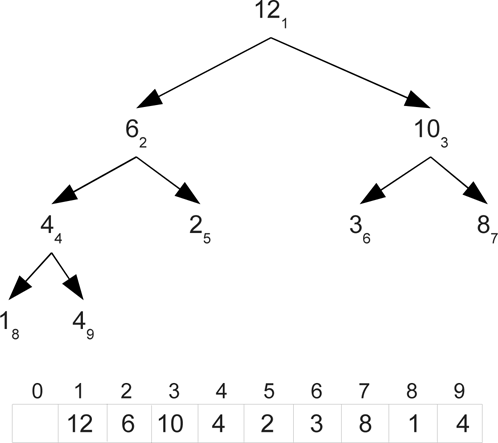
This figure shows the same heap as in figure 32.1 with subscripts that number the nodes in breadth-first order. Below that is an array with the elements at those locations.
The figure shows the array leaving the 0 index spot empty. It is possible to implement a heap with all the elements shifted down one spot so that there is not a blank. However, this requires putting +1 and -1 in the code at many different points. This complicates the code making it harder to understand and maintain. While it removes a little waste in memory, it introduces an overhead in every call on the priority queue. For that reason, and to keep the code simpler, the implementation shown here will leave the first element of the array as a default value.
32.2 Heaps as Priority Queues
To use the binary heap as a priority queue we have to be able to implement enqueue, dequeue, peek, and isEmpty. The last two are simple, the highest priority element is always the root so peek simply returns it. The isEmpty method just checks if there is anything present on the heap. The enqueue and dequeue are a bit more complex because they have to change the structure of the heap.
We start with enqueue where an element is added to the queue. Adding to a Binary Search Tree (BST) was just a task of finding the proper place to put the new element. For a heap, the job is a bit different. The heap has to remain complete so when a new element is added, there is no question about what set of nodes have to be occupied. The next open space in the row that is currently filling in or the first in the next row when the lowest row is complete has to be filled. However, the new element might not belong there. The way we deal with this is to put a "bubble" in the position that has to be filled and let it move up until it reaches the location that the new element belongs. As long as the new element has a higher priority than the parent of the bubble, the parent is copied down and the bubble moves up. An example of adding a new element with a priority of 9 to the example heap is shown in figure 32.3.

Adding a new element with a priority of 9 to the heap shown in figure 32.1 goes through the following steps. A bubble is added at the next location in a complete tree. It moves up until it reaches a point where the new value can be added without breaking the heap-order.
A call to dequeue should remove the element from the root of the tree as that will always have the highest priority. However, to keep the tree complete, the location that needs to be vacated is at the end of the last row. To deal with this, we pull the last element out of the heap and put it in a temporary variable then put a placeholder we will call a "stone" at the root. This stone then sinks through the heap until it gets to a point where the temporary can stop without breaking heap-order. When moving down through the heap there is a choice of which child the stone should sink to. In order to preserve heap-order, it has to move to the higher-priority child as we are not allowed to move the lower-priority child into the parent position above its higher-priority sibling. This process is illustrated in figure 32.4.
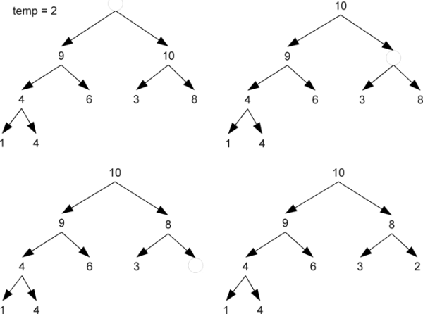
Calling dequeue on the heap at the end of figure 32.3 forces the tree to go through the following steps. The last element is moved to a temporary variable and a stone is placed at the top of the heap. This stone sinks down until it reaches a point where the temporary can stop without breaking heap-order. The stone always sinks in the direction of the higher-priority child.
Code to implement these operations using an array-based binary heap is shown below. This extends the PriorityQueue[A] type that was created in chapter 26. Like the sorted linked-list implementation, a comparison function is passed in to provide the complete ordering of elements for instances of this class. The only data needed by this class is an array we call heap and an integer called end that keeps track of where the next element should be added. These are created with 10 elements to begin with, one of which will never be used as index zero is left empty, and the other is set to be 1.
package scalabook.adt
class BinaryHeapPriorityQueue[A : Manifest](comp: (A,A)=>Int) extends
PriorityQueue[A] {
private var heap = new Array[A](10)
private var end = 1
def enqueue(obj:A) {
if(end>=heap.length) {
val tmp = new Array[A](heap.length∗2)
Array.copy(heap,0,tmp,0,heap.length)
heap = tmp
}
var bubble = end
while(bubble>1 && comp(obj,heap(bubble/2))>0) {
heap(bubble) = heap(bubble/2)
bubble /= 2
}
heap(bubble) = obj
end += 1
}
def dequeue():A = {
val ret = heap(1)
end -= 1
val temp = heap(end)
heap(end) = heap(0) // Clear reference to temp
var stone = 1
var flag = true
while(flag && stone∗2<end) {
var greaterChild = if(stone∗2+1<end && comp(heap(stone∗2+1),heap(stone∗2))>0)
stone∗2+1 else stone∗2
if(comp(heap(greaterChild),temp)>0) {
heap(stone) = heap(greaterChild)
stone = greaterChild
} else {
flag = false
}
}
heap(stone) = temp
ret
}
def peek:A = heap(1)
def isEmpty:Boolean = end==1
}
The enqueue method begins with a check to see if there is space in the array for a new element. If not, a bigger array is created. As with other similar pieces of code written in this book, the size of the array is doubled so that the amortized cost of copies will be O(1). The rest of the enqueue method makes an Int called bubble that will walk up the heap to find where the new element should go. It is initialized to end, the first unused location in the array. The main work is done in a while loop that goes as long as the bubble is greater than an index of 1 or the parent of bubble, located at index bubble/2, has a higher-priority than the new element. When the loop terminates, the new element is placed at the location of the bubble and end is incremented.
The dequeue method starts off by storing the current root in a variable that will be returned at the end of the method. It then decrements end, stores the last element in the heap in a temporary, and clears out that element with the default value stored at heap(0). A variable called stone is created that starts at the root and will fall down through the heap. There is also a flag variable created to indicate when the while loop should terminate. This style is helpful when the determinant of whether to stop the loop is complex and would be difficult to put in a single line. In this case part of the determination is easy, if the stone has gotten to a leaf, it must stop there. Otherwise, it requires checking the temporary against the child or children to see if the temporary has lower priority than the higher-priority child. That would require a complex Boolean expression that would be hard to read. The use of a flag generally improves the readability and maintainability of the code.
Inside the loop, the first task is determining which child has a higher priority. The check in the while loop condition guarantees that there is at least one. If there is a second, and it has higher priority, it is the one we want, otherwise we want the first child. Then that child is compared to the temp to see if the stone should keep sinking. If it should not keep sinking then the loop needs to stop so flag is set to false. When the loops terminates, the temporary is moved to the location where the stone stopped and the original root value is returned.
Using the image of the tree we can argue that both enqueue and dequeue are always O(log(N)). This can also be argued from the code. The variable end is effectively n. In the enqueue method the bubble starts at end and is divided by 2 in every iteration through the loop. This can only happen log2(n) times before it gets to 1. With dequeue the stone starts at 1 and each iteration it changes to either stone∗2 or stone∗2+1. This too can only happen log2(n) times before stone gets to end.
Testing this code is a simple matter of copying the test for the sorted linked-list priority queue and changing what type is instantiated. It can also be used to improve the performance of any other code that requires only the priority queue interface to operate. For example, the cell division example from chapter 26 could be altered and would gain a significant performance boost for large populations.
Priority Queue with Frequent Removes
Back in subsection 26.2.2, when the sorted linked-list was used for an event-based simulation of collisions, we had to add a method called removeMatches. This method was needed because whenever a collisions between two bodies is processed, all future events involving either of those bodies needs to be removed from the queue. The new velocity of the body will make those events invalid. This method was not hard to add to the sorted linked list implementation and the fact that it was O(n) was not a problem as the enqueue method was also O(n).
In the last chapter we saw how adding spatial data structures can improve the overall performance of a time step from O(n2) to O(n log(n)) or even, in certain ideal cases, O(n). However, the sorted linked-list priority queue will still limit performance to O(c2), where c is the number of collisions in the time step. That number generally does increase with the number of particles so using a sorted linked list is still a potential performance bottleneck.
We have just seen that a heap-based priority queue gives O(log(n)) performance for the main operations, which would provide O(n log(n)) overall performance for the number of elements added and removed. This could provide a significant performance improvement for collisions if we could implement removeMatches on the heap. Unfortunately, removing an element from the heap is O(log(n)) and can not be improved significantly when done in bulk. Fortunately, collision handling has aspects that are predictable and can be used to make an alternate implementation.
What is important about collision handling is that from one time step to the next, the number of collisions is fairly consistent and the distribution of times for collisions is fairly uniform. This points to an implementation that combines arrays and linked lists.1 Let us say that in the previous time step there were c collisions for n particles and each time step lasts Δt time units. We start with an array that spans time from 0 until Δt with c elements that each represent time. The array references nodes for linked lists. There is another array with n elements, one for each particle in the simulation, that also keeps references to nodes. Each node is part of two or three orthogonal doubly-linked lists and stores information about an event. One doubly-linked list going through a node is sorted and based on time. The others are not sorted, represent particles, and there is one for each particle involved. So particle-particle collisions are part of two of these and particle-wall collisions are part of two.
A graphical representation of this structure is shown in figure 32.5. The array across the top is for time. The first cell keeps the head of the list for any events between 0 and . The second is for events between and . The array on the right has one cell for each particle in the simulation and the list keeps track of any collisions that particle is involved in. The lists are doubly linked so that any element can be removed without knowing about the one before it in any given list. This figure is greatly simplified in many ways to make it understandable. In a real situation the number of elements in each array should be at least in the thousands for this to be relevant. In addition, while the vertical lists are sorted and there will be a nice ordering for elements, the horizontal links will often double back around and produce a far more complex structure than what is shown here.
So what is the order of this data structure? Linked lists are inherently O(n) for random access. This includes adding to sorted linked lists. On the other hand, adding to the head of a linked list is O(1). In the worst case, all the events could go into a single, long linked list. That would result in O(n2) performance. Such a situations is extremely unlikely given the nature of collision events. We expect roughly c events that are roughly evenly distributed. That would result in sorted linked lists of an average length of 1 and it should be very rare to have a length of longer than a few. The dequeue operation has to remove all the other events for any particles involved, but that is required by any implementation and the advantage of having doubly-linked lists by particles is that this can be done as fast as possible considering only the nodes involving those particles have to be visited. So the expected time for all operations is optimal. For dequeue is is always O(1), the implementation simply keeps track of the element in the time array that has the first element. The enqueue could be O(n), but we expect O(1) performance because the time lists are short. The removeParticle method will perform O(n) operations in the number of events for that particle, but this too should be a small number.
You might wonder why, if this data structure is so great, it is not used more generally. The reason is that it is not generally good. It requires knowing that there should be about c events, they will all lie in a certain finite time range, and they will be evenly distributed. Change any of those conditions and this structure can be worse than a standard sorted linked list. If you ever wonder why you should bother to learn how to create data structures, like linked lists, when there are perfectly good implementations in libraries, here if a reason why. Library priority queues are typically implemented with a heap. For the general case, that is the ideal structure. Not all problems fit the general case though. In this situation, a heap is probably worse than a sorted linked list and the only way you can get significantly better performance is if you write your own data structure.
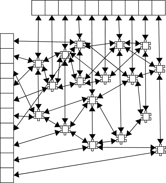
This shows a pictorial representation of the alternate data structure that can be used as an efficient priority queue for collision handling. The top array keeps the heads of lists for different time brackets during the time step. The left array is the heads of lists for different particles. All lists are doubly linked so that nodes can be removed without finding the one before it.
32.3 Heapsort
Any priority queue implementation can be turned into a sort. Simply add all the elements to the queue and remove them. They will come off in sorted order. Insertion sort is roughly what you get if you do this with a sorted array or linked list. The priority queue described in the above aside gives something like a bucket sort. If you build a sort from a heap-based priority queue, you get the heapsort. The fact that the ideal heap uses an array means that heapsort can be done completely in place. Simply build the heap on one side of the array and extract to the other
Here is an implementation of a heapsort. This builds the heap using value as priority so higher values will dequeue earlier. They are then dequeued to fill in the array starting with the end.
def heapsort[A](a:Array[A])(comp:(A,A)=>Int) {
for(end <- 1 until a.length) {
val tmp = a(end)
var bubble = end
while(bubble>0 && comp(tmp,a((bubble+1)/2-1))>0) {
a(bubble) = a((bubble+1)/2-1)
bubble = (bubble+1)/2-1
}
a(bubble) = tmp
}
for(end <- a.length-1 until 0 by -1) {
val tmp = a(end)
a(end) = a(0)
var stone = 0
var flag = true
while(flag && (stone+1)∗2-1<end) {
val greaterChild = if((stone+1)∗2<end &&
comp(a((stone+1)∗2),a((stone+1)∗2-1))>0)
(stone+1)∗2 else (stone+1)∗2-1
if(comp(a(greaterChild),tmp)>0) {
a(stone) = a(greaterChild)
stone = greaterChild
} else {
flag = false
}
}
a(stone) = tmp
}
}
You should notice similarities between parts of this code and the heap implementation. The first for loop contains code that looks like enqueue. The second loop contains code that looks like dequeue. Some modifications had to be made because the array that is passed in does not include a blank element at the front.
This sort is O(n log(n)), the same as for merge sort and quicksort. Unlike those two, the heapsort is not recursive. It is also stable, like the mergesort, and can be done in place, like the quicksort. These factors make it a nice sort for a number of different applications.
32.4 End of Chapter Material
32.4.1 Summary of Concepts
- Binary heaps are one type of data structure that allow quick retrieval of a maximum priority element.
- They are based on a binary tree structure.
- They are always complete and have heap-ordering.
- Numbering tree elements beginning with one going in breadth-first order gives a simple mathematical relationship between indices of parents and children.
- This leads to the most efficient implementation using an array because the heap is always complete.
- Binary heaps can be used to implement efficient priority queues. Both enqueue and dequeue are always O(log(n)) because the heap is a complete tree.
- The heap can be used as the basis for a sort called the heapsort.
32.4.2 Exercises
- Perform a speed test to compare the speed of the sorted list-based priority queue from chapter 26 using a sorted list to the heap version presented in this chapter. Use exponentially spaced numbers of elements to get a broad range of n values.
- Implement a binary heap that does not leave the 0 element empty. Test and debug it to make sure with works.
- If you did the exercise above, you can now do a speed comparison of the heap code in the text to that which starts the heap elements at the zero index.
- The last aside in the chapter describes an alternate implementation for a priority queue that works well for the collision simulation where scheduled events have to be removed regularly. Write code for this and compare its speed to other priority queue implementations that you have.
32.4.3 Projects
For this chapter, you should convert whatever you did in chapter 26 from the implementation you used in that chapter to one of the ones presented in this chapter. For the simulation workbench, if you have done a collisional simulation, consider doing the special priority queue that makes it easy to remove events.