Chapter 12

Modeling a Complex Structure

Tim Danaher

After studying architecture at Bath and Oxford, Tim Danaher took the architectural visualization route, producing 3D perspectives and animations. He has also produced numerous illustrations for the computer press in Great Britain and has written articles on computer graphics and architecture for the Architect’s Journal. At present, he lives in Cologne, Germany, where he teaches courses on design issues and, naturally, SketchUp at KISD (Cologne International School of Design). He is also developing a parallel career as a translator for architecture and design (he translated the chapters of this book that were originally in French).

Project: Lawyers’ chambers, Falkestrasse, Vienna (by Coop Himmelb(l)au)

Tools: SketchUp 7, Cheetah3D 4.7, Photoshop CS, Make Cubic

Project Context

Tim Danaher: “This project was chosen for several reasons: to test the limits of the software (I was sick and tired of hearing people say “you can’t do that with SketchUp!”), to test my own abilities with the software and, hopefully, to learn some new techniques along the way. I also wanted to use the model to test the rendering capabilities of a piece of software that I had not yet used but about which I had heard a lot of good things, Cheetah3D.

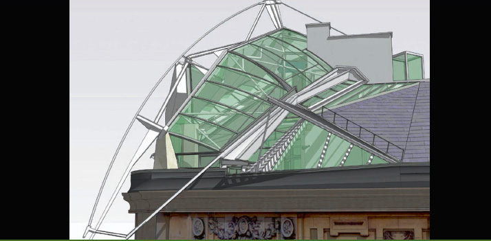
But probably the most important factor that pushed me into modeling this project was a long-held desire to understand the structure: I started at architecture school the same year (1987) that this icon of deconstruction hit the architectural headlines. When you first look at it, it seems impossible to understand – a tangle of cranked beams and glass canopy perched precariously on the edge of a roof. And just how did they make it waterproof?

Using photographs sourced from the Web, I was able to put together a first rough draft, and as I found new photographs or plans, I refined the model bit by bit. The method presented here is necessarily different from the one that I used for the first models, since here I will be using other information that I have gathered over the years, including an original plan and section.

So what did I get from this project? The satisfaction of a job well done (I hope), a mystery solved… but also a little disappointment: I can never look at this wonder again through the same eyes; it has given up (almost) all its secrets to me.

Since this was a private project, there was no deadline. Modeling was carried out as and when time allowed. If there was one major constraint, it was the lack of information: It is difficult to believe that after more than 20 years, there are so few images in circulation of such iconic structure; there is not even a single monograph on it!

I started modeling by studying the images obtained up close. Several attempts were made (including many false starts) before a model was produced that could serve as the basis for further analysis.

All the initial modeling was carried out in SketchUp 5 (the project was started nearly four years ago). Only SketchUp’s basic tool set was used – no modeling plug-ins were used, and only the Bomb.rb Ruby was used to prepare the model for export. The version 5 model was exported to version 4 to make the animations. This got around the well-known “flickering shadows” problem. Version 4 was the only version to avoid this problem. The infamous “shadow problem” came back with version 5, and it is still with us today. All the textures were applied in SketchUp, with Cheetah3D providing features like lighting, rendering, camera animation, and panorama preparation. Apple’s free MakeCubic.app was used to process the panoramic images into QTVR panoramas. Photoshop was used in the preparation of some of the textures and also in scanning and preparing the plan and section.”

Why Choose SketchUp?

SketchUp was chosen for its speed and its fluid modeling ability. It was also chosen because previous attempts to build this with two traditional modeling heavyweights – LightWave and form•Z – had to be abandoned in desperation. The idea was that SketchUp’s simpler approach might not get in the way – something that proved, indeed, to be the case.

Cheetah3D – a full-featured 3D modeling, rendering, and animation application – was chosen for postprocessing because of its unequaled render management and its blazingly fast, multitasking, multi-processor, hyperthreading rendering engine. It was also chosen because of the speed with which it can produce QTVR panoramas. After long days (and nights) of modeling, I did not want to have to wait a couple of days more for the results of a camera animation. Rendering a QuickTime panorama can be done in minutes with Cheetah. Also, it exchanges data with SketchUp very easily thanks to its FBX format support and Smart Folders feature. Oh, and did I mention that it costs only $149?

Techniques Used

As previously stated, only SketchUp’s basic modeling tools were used in this project. However, probably more important than SketchUp’s tools were observation, reflection, and a lot of head-scratching. A two-monitor setup also helped, with a second monitor dedicated to displaying the drawings and photographs that needed to be consulted constantly. The second monitor usually holds all of SketchUp’s palettes, so a shortcut was assigned to the Hide Dialogs command (from the Menu Bar, choose Windows > Hide Dialogs), enabling all of SketchUp’s floating palettes to be hidden or displayed with a single key press.

Great use was made of the Outliner palette for organizing this model (I have a motto: Group early, group often). For a model as complex as this one, clear organization is of the utmost importance. I use Layers: they just confuse me.

New Approaches

In this model, certain elements were built in free space – something that is not the usual approach in SketchUp. It was necessary to fake a feature that exists in almost all other modeling programs: working planes. These are virtual surfaces – normally defined by three coplanar points – that allow you to draw in “midair.” Normally, in SketchUp, you can only draw upon already existing surfaces, so the approach here was to draw some simple faces and then move and rotate them until they were in the correct position. They would then act as virtual “drawing boards” on which most of the main structure could be drawn in situ. Drawing these main structural elements orthogonal to the X, Y, and Z axes and trying subsequently to rotate them into place would have been a recipe for disaster.

Stage 1: Preparing a 1:1 Scale Plan

Objectives: To bring together all the photographs, plans, sections, and axonometrics from various sources (by downloading, scanning, etc.) and ensure that the imported plan and section are at 1:1 scale.

Data: JPEG images.

Tool: SketchUp Pro.

After the two JPEG scans of the plan and the section were imported, the first problem was one of scale: They both needed to be at 1:1, since a lot of the modeling was going to be eyeballed and having everything at true scale meant there would be one thing less to worry about. Once the plan was imported (where the plan’s size was arbitrarily set), a feature on the drawing was chosen whose dimensions were known (more or less). In this case, the feature was a door opening, and it was assumed that it would be around 2' 9" wide. A line was drawn across this door opening, and then the Tape measure tool was used to measure the line. The value for this line length appeared in the VCB, and then it was simply a matter of typing in the real-world measurement. At this point, SketchUp asks if you want to rescale the whole model. Click on OK, and the plan will now be at 1:1 scale (you can verify this by using the Tape Measure tool to measure the line just drawn).

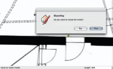
FIG 12.1 The Rescale dialog box.

Stage 2: Constructing the Base Building and Placing the Section

Objectives: To construct a floor of the original building to act as a base and to place the section.

Data: Scale plan obtained in stage 1.

Tool: SketchUp Pro.

The original building and the existing partition walls were constructed by tracing over the imported plan, whereas the cornice was modeled using the Follow Me tool. The main building structure and the interior partition walls were then assigned to different, named groups. The next stage was importing the section, and then placing it in the correct position on the model. This was rather tricky and had to be eyeballed using features that appear on both the plan and the section. In this case, the stairs and the Beak of the main girder were used.

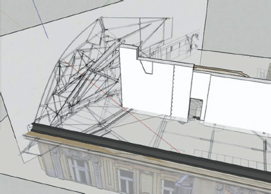
FIG 12.2 The section and the plan in place on a textured model of the original building.

Stage 3: Constructing the Path of the First Girder on Plan

Objectives: To construct the “scaffolding” for the path of the first girder.

Data: The model obtained in stage 2.

Tool: SketchUp Pro.

The problem that now needs to be confronted is that all the girders in the construction are “cranked”: They are bent both on plan and elevation. Working planes now have to be constructed that will allow the paths of the girders to be drawn in situ. As previously stated, drawing a straight girder and then trying to bend it will get you nowhere.

The first step is to draw the path of the girder on the plan. What we are trying to achieve here is a simple vertical face bent at some point along its length. Unfortunately, SketchUp does not allow you to extrude simple lines, so a 2D surface containing the bent line must be created and then Push/Pulled to the required height. This produces a volume, but only a simple surface is required; so any unwanted edges can simply be deleted using the Eraser tool. Group the working plane and give it a name.

FIG 12.3 The profile of the first girder traced on plan: Extrusion of the profile with Push/Pull is followed by the removal of unwanted edges.

Stage 4: The Construction of the Path of the First Girder on Elevation

Objective: To construct the “scaffolding” for the profile of the first girder.

Data: Model obtained in the previous stage.

Tool: SketchUp Pro.

The first step is to reduce the opacity of the working plane surface, so that the section can be seen behind it. Then, starting on either the left- or the right-hand edge of the surface, the path of the girder is traced using the Line tool, making sure that the line drawn adheres to the surface (SketchUp’s inferencing engine should do this automatically: Look out for the On Surface tooltip). The working plane surface can now be deleted or hidden; only the line is needed for the next stages. Use the Orbit tool here to verify that the line follows the path of the girder both on plan and on elevation (see Fig. 12.4).

FIG 12.4 Construction of the profile on the surface of the working plane: Final profile, showing the crank in two planes.

Stage 5: Extruding the First Girder

Objective: To create the 3D form of the first girder.

Data: Model obtained in the previous stage.

Tool: SketchUp Pro.

Next, a suitable girder cross section was chosen from the Components library (Components palette > Construction > Steel Cross-Sections > Wide Flange). It was positioned using the Move and the Rotate tools. One problem is that components align themselves either to the principal axes or to the geometry of the model, which can often mean that once they are placed they lie “flat on their back.” Luckily, since version 6, you can define an axis of rotation simply by clicking and dragging between two points with the Rotate tool. This makes rotation of off-axis groups or components much easier.

Once the girder profile was in the correct position in relation to the path, the Follow Me tool was used to extrude it along the path. And there you go. Now the girder just needed to be grouped and named.

FIG 12.5 The girder profile in situ: The girder is created with the Follow Me tool.

Stage 6: Modeling the Other Main Girders

Objective: To finish the modeling of the remaining simple girders.

Data: Model obtained in the previous stage.

Tool: SketchUp Pro.

Exactly the same technique was used to model the remaining girders. In Figure 12.6, they have each been given a different color, to better distinguish them.

FIG 12.6 The four main girders in situ.

Stage 7: Additional Modeling on the Main Bow Truss

Objective: To add more details to the main girder using working planes.

Data: Model obtained in the previous stage.

Tool: SketchUp Pro.

To add supplementary modeling of the bow truss to the main girder, additional working planes had to be constructed. Using the Axis tool, the red, green, and blue axes were aligned with the top surface of the upper flange of the lower part of the main girder. Use of the Axis tool, rather than the right-click method used in stage 6, verifies that the axes are perfectly aligned with the flange surface. The results of the right-click method can sometimes be not quite what you are expecting. Next, a working plane was constructed perpendicular to the top flange of the girder, simply by drawing in the new green and blue axes. The same method was used to construct a working plane for the upper part of the girder.

The path for the upper triangulating girder is a bit complicated: The working plane was built on the external edge of the upper flange, but the path for this element should start on the internal edge of the upper flange. The next two clicks (where the middle strut would be built) should be on the working plane itself. Then, the end of the line should terminate on the external edge of the upper flange of the upper part of the girder. Care needed to be taken here that the end of the line does not stick to any other surface in the model (e.g., the section). This was a bit of a painstaking procedure; but because of the slight kink in the main girder, it was impossible to put a planar triangulating girder in place. Once the path was drawn, the triangulating girder was extruded using the Follow Me tool (see Fig. 12.8).

FIG 12.7 The constructed working plane in place: Note the position of the axes.

FIG 12.8 The triangulating girder after its extrusion using the Follow Me tool: The line starts on the interior edge of the girder. Points two and three are on the working plane itself, and the fourth point terminates on the external edge.

Next, three additional elements were constructed. These were given nicknames in order to be able to refer to them more easily: the Beak, the Pawn, and the Swim Fin (see Fig. 12.9). These elements were constructed using the two working planes and the section, and – in conjunction with the working planes – they serve as guides for the construction of the bow. The path for the bow was constructed in two stages, starting with the Beak and constrained to the lower working plane, then up to the position of the Pawn strut (first arc), then toward the upper part of the Swim Fin (second arc), and finishing with the end of the arc constrained to the upper working plane (you should see the On Surface tooltip). Again, care has to be taken with the paths of these two arcs to avoid any kinks in the middle. Once the path was complete, a circle was extruded along it using the Follow Me tool to complete the bow.

FIG 12.9 The completed main bow truss.

Stage 8: Modeling the Lower Part of the Glass Canopy

Objective: To model the main glazing using the Push/Pull tool and working planes.

Data: Model obtained in the previous stage.

Tool: SketchUp Pro.

A working plane was constructed (yes, another one) for the panes of the lower part of the central glass canopy, bounded by the two girders on either side of it (the white and pink girders in Fig. 12.6). The axes were aligned with the central web of the main bow truss girder, and the working plane was drawn and rotated into place, scaling it as required so that it fits between the two main girders. The position of this working plane was determined by the bend on the main bow truss girder and the Shark Fin protrusion on top of the other main girder (see Figs. 12.6 and 12.11). The angle of the working plane was judged by eye, using the photographic material already collected.

FIG 12.10 The working plane used for the construction of the canopy profile: The profile is drawn on the working plane.

The canopy profile was now drawn on the grouped, locked working plane. The curve of the canopy profile was eyeballed from the photographs and a closed surface was created, since in the next step we would need to use the Push/Pull tool. The lower part of the canopy is composed of five panes, so the correct value was arrived at by dividing the length of the lower part of the main bow truss girder by five. The canopy profile was Push/Pulled by this amount to create the first pane.

The remaining four panes were created by using the Push/Pull tool on the first pane extrusion, but by double-clicking while holding down the Ctrl key (for Microsoft Windows) or the Alt key (for Mac). This applies the same Push/Pull offset as in the previous operation, creating a new segment each time. Doing this four times gave the required five panes. The canopy geometry was then grouped and named.

This is where the process got a bit tricky: The canopy needed to be rotated into place so that it lay between the two main girders. This required quite a few rotations to find the right spot (see Fig. 12.12).

FIG 12.11 The canopy after extruding it multiple times with the Push/Pull tool.

Once the canopy was finally in its correct position, the overlapping edges needed to be trimmed using the Intersection tool. The canopy group was entered, and all the geometry inside was selected by triple-clicking it and then right-clicking to give Intersect > Intersect with Selection. The unwanted geometry was then simply trimmed using the Eraser tool (see Fig. 12.13).

FIG 12.12 The canopy in position (after quite a few rotations).

FIG 12.13 The canopy after trimming it with the Intersection and Eraser tools.

Next, some more detailing was carried out: Mullions were added by using the Follow Me tool, using the curves between each canopy segment as a path. This was done using a copy of the canopy glazing, positioned using the Edit > Paste in Place option and keeping the original hidden. Once the mullions were constructed, the glass in this copy of the canopy could simply be deleted, leaving the mullions in their own group that was separate from the original canopy glazing group. The upper canopy was built using the same technique as the lower. All the difficulty in constructing this model resides in getting the relationships between the central glazed canopy and the main girders correct. After that, in comparison with the other steps, everything is plain sailing.

FIG 12.14 The mullions and some additional glazing structure in place.

FIG 12.15 The final model.

The final result can be seen in Figure 12.15. This model represents maybe three months of work spread out over a period of three years.

Stage 9: Preparing the Model for Export from SketchUp

Objective: To prepare the model for export.

Data: The completed 3D model.

Tools: SketchUp Pro, Bomb.rb.

As soon as the model was completed, a copy was made and the Bomb.rb Ruby plug-in was run on it. This plug-in explodes every group and component in the model, leaving only the edges and surfaces (the so-called raw geometry). Depending on the complexity of the model, this can take a while: Certainly, there was plenty of time to go and make – and drink – a cup of coffee. For this model, it took around an hour. Next, all the surfaces were grouped according to their material. To do this, right-click on a surface and choose the option Select > All with Same Material. The selected surfaces were then grouped, named according to material, and then hidden. When you cannot see any more geometry in your model, you are done.

FBX was chosen as the export format. From the Menu Bar, choose File > Export > 3D Model … > FBX. In the Export Options dialog, make sure that only the Export Texture Maps and Swap YZ Coordinates (Y is up) tick boxes are checked. This last option is important, since SketchUp, like all CAD programs, treats the blue (Z) axis as “up,” whereas Cheetah, like all digital content creation applications, treats the Y axis as up.

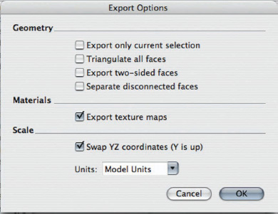
FIG 12.16 SketchUp’s Export Options dialog box.

Stage 10: Importing the Model into Cheetah3D

Objective: To import the FBX file into Cheetah using a Smart Folder.

Data: FBX file obtained in stage 9.

Tool: Cheetah3D.

If you have a Mac, Cheetah3D (available at http://www.cheetah3d.com) is the perfect partner for SketchUp. This extremely capable 3D program has an incredibly fast rendering engine – one that has become even faster since the release of version 5. This is due to the fact that it can utilize all the cores of the Mac’s CPUs and now makes use of the hyperthreading capabilities in Intel’s new chips. With an 8- or 12-core Mac Pro, rendering speeds that were unthinkable only a few years ago can be achieved. The rendering engine also supports the Radiosity/Ambient Occlusion and high dynamic range image (HDRI)/Global Illumination lighting models for an unequaled level of realism. Render management is also extremely well thought out: The number of simultaneous renders (even from different scenes) is only limited by the available RAM in your computer, and all completed renders and those that are being currently calculated are shown in a graphical browser.

Before importing the model into Cheetah, a Smart Folder was created. Smart Folders are one of the greatest advantages of Cheetah for SketchUp users, since they create a pipeline between the two programs. Placing an FBX file (or 3DS or any other format) into a Smart Folder means that every time the model is changed in SketchUp and reexported, the copy in Cheetah will update automatically to reflect those changes.

FIG 12.17 Cheetah’s Smart Folder feature makes the management and updating of exported models easy.

FIG 12.18 Parameters for the Area light in the Cheetah scene.

Stage 11: Setting Up the Initial Lighting in Cheetah3D

Objective: To create a photorealistic rendering using Radiosity and HDRI illumination.

Data: Cheetah scene created in stage 10.

Tools: Cheetah3D, Photoshop (optional).

As is always the case, lighting is the essential step in obtaining a convincing rendering. An Area light and an HDR image were chosen as the principal sources of illumination, combined with Radiosity rendering. This combination provides very natural lighting; the shadows in particular have an extremely real feel to them with natural, soft edges. Luckily – and completely by accident – the Area light was placed so that the shadow direction in the Cheetah scene corresponded almost exactly to that in the SketchUp scene. The Area light setup can be seen in Figure 12.18.

Although the choice of an Area light is essential for proper lighting, falloff, and shadows, an appropriate rendering technique must also be chosen to ensure best results. Cheetah’s rendering engine is basically a raytracer at heart, but this technology is taken to another level by the incorporation of two further technologies: Radiosity and HDRI/Global Illumination. Radiosity is a technique that simulates very accurately the effects of diffuse and scattered light, whereas HDRI/Global Illumination uses HDR images as a source of illumination. The combination of these two techniques is able to produce images of the very highest quality. Of course, there is always a compromise: In this case, it is an increased rendering time (although the multicore, hyperthreading capabilities of the renderer do much to mitigate this).

In Cheetah, all the rendering setup is done through the Camera object, and the number of cameras that you can have in any one scene is practically limitless. Each camera in Cheetah is basically a raytracing engine that can be augmented by the addition of “tags.” In Figure 12.19, from left to right these are Camera, Radiosity, and HDRI.

FIG 12.19 Camera object with Radiosity and HDRI tags attached.

Clicking on each tag reveals the setup options: For Radiosity, the most important option is Type. Here, you can choose between Radiosity and Ambient Occlusion. The latter produces results that are almost indistinguishable from Radiosity, but with significantly faster rendering times. The other two parameters that need to be noted are Intensity (brightness) and Samples. The Samples parameter is particularly important, because the higher its value, the fewer rendering artifacts there will be in the final image – but, of course, rendering time will increase. Values of around 150–200 produced the best trade-off between quality and rendering time for this project. Values of around 40 were used to run quick lighting test renders.

FIG 12.20 Choosing Ambient Occlusion reduces rendering time: Typical values for Radiosity are shown.

To set up the HDRI render, a file in .hdr format needs to be loaded into the HDRI tag. Images with the .hdr extension are high dynamic range images. They contain 32 bits per R, G, and B channels, as opposed to the standard 8 bits for formats such as JPEG and TIFF. Since the primary source of illumination in this model is daylight, an image of a partially covered sky was chosen. If the image is already in .hdr format, so much the better. If not, and if you have a Photoshop license, you can convert any 8-bit image to .hdr format in the following manner: From the Menu Bar, choose Image > Mode > 16-Bit, and then Image > Mode > 32-Bit. This has to be done in two stages, because 8-bit images cannot be converted directly into 32-bit images.

FIG 12.21 Setting up the HDRI tag.

For architectural projects, Panoramic projection for the HDR image is the correct choice in 99% of the cases: It avoids any “seams” in the image when it is used as a backdrop to the scene. The values for the Power and Clamp Power parameters will be different for each scene, according to the already existing illumination, the intensity of the Radiosity setting, etc.

After several attempts, a satisfactory initial lighting setup was achieved (this is the product of the illumination from the Area light and from the HDR image; see Fig. 12.22).

FIG 12.22 Initial lighting: The shadow quality is extremely convincing.

Stage 12: Setting Up Supplementary Lighting in Cheetah3D

Objective: To set up accent lighting for the interior shots.

Data: Cheetah scene created in the previous stage.

Tool: Cheetah3D.

At first glance, the interior illumination seems to be pretty simple: The main source of illumination is the sky and the sun. This may be true, but there are light sources everywhere in the space itself that add ambience, accent, and atmosphere – probably around 40 in total, and among them are spotlights, uplighters, and neon tubes. In Figure 12.23, each red spot represents a single luminaire. You can see the results of all this combined lighting in the second picture.

FIG 12.23 Position and number of (some) supplementary light sources: A new scene with supplementary lighting in place is shown.

Stage 13: Generation of a QTVR Panorama in Cheetah3D

Objective: To generate a QTVR panorama to enable the viewer to look around the interior space.

Data: Cheetah scene created in stage 12.

Tools: Cheetah3D, Apple MakeCubic.app.

The greatest advantage of making a QTVR panorama is the speed with which usable results can be obtained. Although the calculation of a frame-by-frame animation can take days, a fully navigable QTVR panorama that lets the viewer look around the entire space may take only a quarter of an hour to generate.

To generate the panorama, the Panorama projection was chosen for one of the cameras in the Cheetah3D scene. The location of the camera will determine the pivot point about which the QTVR panorama turns; so a camera was set up in the middle of the space to give a good, all-around 360° view. The height of the camera also influences the view obtained; so this camera was set at 5' 6" off the ground (average eye height). It was then just a matter of clicking Cheetah’s Render button and waiting for the result.

Once the render was complete, an image like the one shown in Figure 12.25 was obtained.

FIG 12.24 Setting up a Cheetah camera to record a panorama.

FIG 12.25 The panoramic image produced by Cheetah’s camera.

The next step is to turn this panoramic image into a fully navigable QTVR panorama. To do this, Apple’s own MakeCubic.app was downloaded, started up and the image obtained in stage 12 was loaded into it. Although MakeCubic’s interface is – it must be said – a little antediluvian, it does the job quickly and is free. By sticking to the default configuration, a navigable panorama was obtained with just two clicks of the mouse (from the Menu Bar choose File > Convert, then click OK in the dialog box that appears; see Fig. 12.26). Another option is to simply drag and drop the panorama onto MakeCubic’s icon.

FIG 12.26 Setting up MakeCubic.

The QTVR panorama can now be viewed in Apple’s QuickTime Player.app. More can be found at http://vizarch.blogspot.com

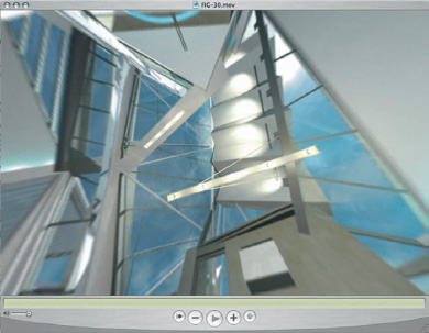
FIG 12.27 Navigating the QTVR panorama in Apple’s QuickTime Player.