
IN THIS CHAPTER
Understanding databases
Configuring data source names
Using Microsoft Query
Creating PivotTables
Using Goal Seek
Working with Scenarios
Today's Information Technology-driven offices have one thing in common: They all tend to have lots of different types of data that need to be processed. Whether it's bookkeeping, trend analysis, sales information, or basically anything, it seems that every bit of data is stored in a database for use and archival purposes.
Although Excel itself isn't really a database (at times it can almost pass for one), its variety of functions and features for working with tabular data makes it a natural complement to one. If you find yourself having to crunch numbers often, you'll find Excel's ability to pull data right from a database to be invaluable. Excel takes advantage of the power of Structured Query Language (SQL), the standard language of relational databases, to build queries that can encompass data spread over multiple relational database tables, join the data, and bring it into an Excel workbook for your use.
In this chapter, you learn how to configure Excel 2008 to use Open Database Connectivity (ODBC) to make a connection to a remote database. You also see how to use Microsoft Query to build the database request and retrieve data into a worksheet. Once there, you see how to make the best use of the data by using PivotTables, Goal Seek, and Scenarios to analyze it.
Finally, this chapter shows you some other Excel 2008 data analysis tools that can help make your number-crunching tasks faster and easier. You learn how to use Goal Seek to work backward to find data values and how to use the Scenario Manager to let Excel run various test cases into your formulas and summarize the results.
Databases come in all shapes and sizes. There are huge enterprise-class databases with many gigabytes of storage, two of the most popular being Oracle and Microsoft SQL Server. There are medium-sized open source databases such as MySQL and PostgresSQL that drive cost-conscious businesses and legions of Web applications. And there are smaller, desktop-class databases such as Microsoft Access and FileMaker Pro, which are used for smaller data storage and analysis tasks.
No matter the size, and how differently they are designed, most databases have some things in common. For example, some standards have evolved over the years for database connectivity. Many databases offer a "native" interface that allows clients to gain efficiency by connecting to them directly, but the disadvantage of this is that each application must know how to make the native connection. This puts the burden on database makers and application developers to create drivers so the products can talk to one another.
To solve this, a standard for database connectivity was created to provide a middle ground. Open Database Connectivity (ODBC) was designed by the SQL Access Group in 1992 to give database makers a standard interface to their products that any application can use. From the application point of view, adding ODBC support means they can automatically take advantage of any database that provides such an interface.
Excel 2008 can use its ODBC connectivity to retrieve data from any number of databases, so long as the database provider (or a third-party) provides an ODBC driver that works with the Macintosh's operating system. Fortunately, drivers for all of the most popular databases are available, and in many cases you have more than one option.
While drivers can come from a variety of vendors and third-party providers, after they are installed, you can create Data Source Name (DSN) entries to control access to a particular database in the ODBC Administrator utility, which can be found in your Applications/Utilities folder. Although a thorough explanation of this utility is outside the scope of this book, any driver that you purchase or download should have instructions for installing and configuring connections and likely makes use of this or a similar ODBC administration tool. Figure 17.1 shows the ODBC Administrator at work.
The two main types of DSNs that you can use with Excel are System and User. A User DSN can be used only by the user who sets it, which in most cases will be you. A System DSN, on the other hand, can be used by any user account that is set up on your computer. If you are the only user on your computer, the distinction may not seem important, but if others use your system and also need to be able to access the database, then you are better off creating a System DSN unless there is a specific reason to deny other users access. The following steps are typical in defining a database connection, in this case using the OpenLink driver to talk to a MySQL database:
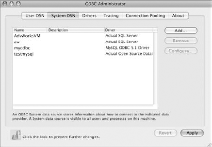
Figure 17.1. You can use the ODBC Administrator to configure Data Source Names that point to your database.
Locate and install an ODBC driver for your database.
Open the ODBC Administrator (in Applications/Utilities).
If necessary, unlock it by clicking the lock icon in the lower-left corner and entering your administrative password.
Click the System DSN tab.
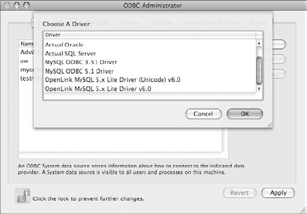
Click Add.
Choose the appropriate ODBC driver from the provided list, shown in Figure 17.2.
Enter the connection information for your database. Every database type and driver has its own setup wizard, but most ask you to enter a DSN name, connection information including a hostname or IP address, ports, and a username. Figure 17.3 shows a typical one.
You also may be asked to provide a password, but this is typically used only in the setup to obtain information from the database and then to test the connection.
Some drivers have many connection options, some are simpler. In general, you should leave settings at the default values unless you know what you are doing or have specific instructions from a database administrator.
Most driver setup wizards have a way of testing the connection at the end of the process, so verify that everything works before clicking the Finish button.

Excel is capable of importing data from a variety of sources, including database and various file formats. In Chapter 13, you learned about the basics of importing some types of external data, including from text files, CSV files, and FileMaker Pro databases. Now you learn how to import directly from an ODBC connected database into Excel. After you have a database driver installed and a DSN configured, you're ready to begin.
To retrieve data from a relational database, you have to first be able to define the tables and query parameters to retrieve it. Relational databases consist of one or more tables, each of which may have data that relates to another table. For example, you could have a table containing Orders, with fields (called columns in database parlance) that contain an order date, product number, quantity, and other relevant information, including a customer ID. The customer ID would relate to another table called Customers, which could contain information such as addresses and phone numbers. The Structured Query Language (SQL) was designed to be able to work with relational data, and it has numerous options for building queries.
Explaining how to make queries using SQL syntax is beyond the scope of this book; in fact, entire books have been written just on this subject. Fortunately, you don't need to learn SQL in order to import data into Excel, because Microsoft thoughtfully included a tool called Microsoft Query, which lets you easily create queries and test them visually. (If you happen to know SQL, you are, of course, free to use it.)
Learning how to work with Microsoft Query is the key to mastering Excel's data importing power. But first, you need to tell it which data source you want to use. Follow these steps to get started:
In Excel, choose Data
Get External Data New Database Query.
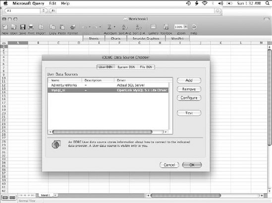
This launches the iODBC Data Source Chooser dialog box, which is a bit like a stripped-down version of the ODBC Administrator tool you used to create the data source. In fact, if you somehow skipped that step, you can do it from here, as well. (Add, Remove, Configure, and Test buttons are available here that you can use to manage your DSNs.) Figure 17.4 shows the Data Source Chooser dialog box.
Click the tab of the DSN type you created: User, System, or File.
Click the data source name.
Click OK.
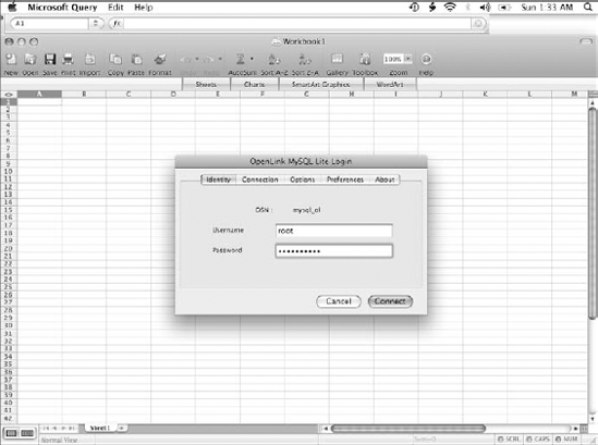
At this point, you likely will be asked for authentication information in the form of a username and password to access your database. Figure 17.5 shows an example, but yours may look different depending on the ODBC driver you are using. See the documentation that came with your ODBC driver if you have questions about what to enter here.
Enter your username and password, and click OK (or Connect, depending on your driver).
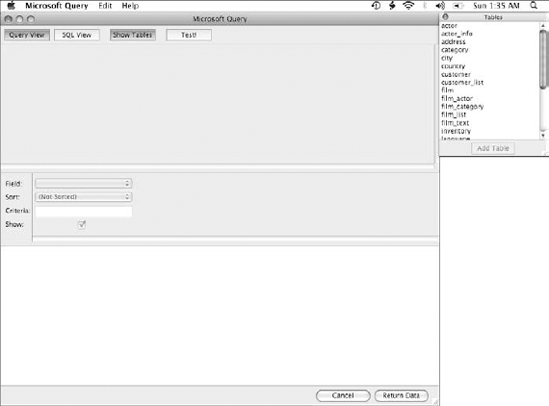
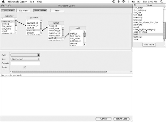
If all went well, you should now be in Microsoft Query with a floating palette of tables, similar to that shown in Figure 17.6. (Of course, the tables in your database will be different!)
At the top of the Microsoft Query menu, you see four buttons, which are the main controls for working with queries:
Query View: Use this view when you want to construct a query visually, using boxes and lines to show tables and references.
SQL View: Use this button to toggle the view to SQL view, where you can see the SQL statement that your query is using. You can edit the SQL statement directly if you prefer.
Show Tables: This can be used to open the Tables Palette again if you happen to close it.
Test!: Run the query as it currently exists. If successful, you see the data you import displayed in the lower portion of the screen.
Below the buttons, a portion of the screen is reserved for displaying either the selected tables or the SQL code depending on the view you select. Under that are controls for working with data that you retrieve (the Fields pane). The lower portion of the screen is reserved to show data retrieved using the Test! button (the Data pane).
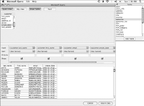
The easiest way to create a query is to use the Query view. Click that button, and open the Tables Palette if it's closed. Then follow these steps:
Click a table name in the Tables Palette to select it.
Click Add Table.
A box with the fields (or columns) in the table is displayed in the Tables pane. You can drag this box around within the window if you like.
Select fields to retrieve in the query by double-clicking them.
Fields appear in the Fields pane as you double-click them.
The first field listed in every table is the * wildcard. This can be used to include all fields in the query.
Repeat Steps 1 through 3 for any additional tables or fields you want to include in the query.
Click Test! to run your transaction. The data matching your query should be retrieved and displayed in the Data pane, similar to that shown in Figure 17.7.
If after adding tables and fields to a query you decide you don't want them included any more, it's easy to remove them.
To remove a field from the Fields pane, right-click or Control+click in the field box, outside of any of the controls. Then choose Delete.
Tables can be removed from the Tables pane in the same way. Right-click or Control+click on a table, and then choose Delete.
Although it's possible that you want to retrieve all the data in the tables that you've chosen, it is more likely that you'd like to refine the query and restrict it to only retrieving the values that you like. You can accomplish this in two ways. One is by specifying criteria for chosen fields to limit the values that can be retrieved. The other way is to create joins between tables.
In the Fields pane, you may have noticed the Criteria field. This field can be used to limit the records returned by a query by specifying criteria that a particular field must match. Every potential record retrieved is evaluated against all the criteria. If it doesn't match any of them, the record is excluded from the results.
Figure 17.8 shows a sampling of data from the Sakila database's film_list view, which is used as an example for the various criteria options.
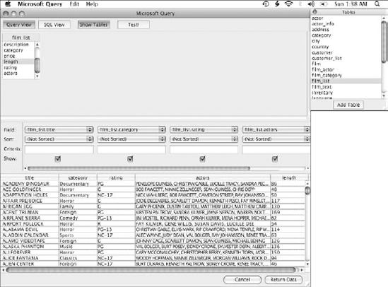
The following are some examples of criteria you can specify to restrict data from the film_list table:
You can use the LIKE operator to restrict data to that which matches a partial string. For example, you can restrict the film_list query to only include movies that being with the letter A by using LIKE 'A%'. Criteria text must be enclosed in single quotes. The % character is a wildcard character meaning that the results can include titles that start with 'A' followed by any other text. Likewise, LIKE '%KIRSTEN PALTROW%' applied to the actors field would limit the query to movies with that actress in the cast.
You can use mathematical operators such as equals (=), greater than (>), greater than or equal (>=), less than (<), less than or equal (<=), and does not equal (<>). These operators can be used on numeric, date, and text fields. > 120 applied to the length field would retrieve movies longer than two hours. Likewise, you can retrieve movies in the Horror category by applying = 'Horror' to that field.
You can use the IN operator to match a field to values in a list. For example, you can limit results to PG-13 rated movies or higher using this criteria applied to the rating field: IN ('PG-13', 'R', 'NC-17').
You can find records that are missing data. Use the IS NULL operator in the criteria box for a field to retrieve records with null values in the field.
You can use the NOT operator in front of most of these criteria to negate the results. For example, NOT LIKE '%KIRSTEN PALTROW%' applied to the actors field returns all movies that don't include her in the cast.
If you add individual fields rather than the * wildcard, you can specify a sort order for your fields. Sort orders are applied from left to right. Options include no sorting (in which case data is retrieved in the order that it exists in the database table), Ascending (from lowest to highest, numerically or alphabetically), or Descending.
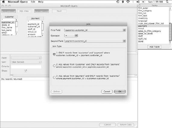
If your query includes data from multiple tables, you can refine the query in another way: You can create joins between tables. Joins are key to the power of a relational database, because they are used to define the relationship between one table and another. You can create several types of joins, and the type you choose is important to ensure that your query returns the correct results. To create a join, do the following:
Click a field in a table in the Tables pane.
Drag the field name to another table.
The Join dialog box appears, as shown in Figure 17.9.
If the fields you are joining have the same name, Excel automatically adds it to the Second Field box; if not, choose a field to use for the join comparison from the list.
Choose a join operator. In most cases, you can leave this as the default value of Equals (=), but you can use other operators to join based on unequal relationships between the fields as well.
Choose the join type. The default choice, item 1, specifies an inner join where both tables must have matching fields. Options 2 and 3 are used to specify outer joins. Inner and outer joins are explained in more detail below.
Click OK. The Tables pane now shows a line between the joined fields indicating the relationship, as shown in Figure 17.10.
You can edit or delete a join by right-clicking (or Control+clicking) the join line in the query view. The two types of joins are described here:
Inner join: The default type of join, an inner join selects records where the joined fields in both tables match. If one record doesn't have a matching record in the other table based on this field, neither record is included in the results. Figure 17.10 shows an inner join between the inventory.film_id field and the film_list.FID field. A result set using an inner join can include multiple entries for each record, because you can have many records in each table matching.
Outer join: An outer join selects all the records from one table regardless and includes records from the second table when a match exists. When a record from the table that's contributing all its records can't be matched with a record from the other table, the record still appears in the result set. Empty cells are used in place of data when no matching record is found in the other table.
When you have a query defined the way you want it, you can return it to Excel by clicking the Return Data button. Click this button to open the Return External Data to Microsoft Excel dialog box, shown in Figure 17.11. This dialog box tells Excel where to put the new data.
Choose one of the following options for returning data:
Existing sheet: The data is inserted into the existing sheet starting at the specified cell. You can choose a different starting cell by using the collapse button and selecting a cell or a range of cells.
New sheet: Excel creates a new worksheet and inserts the data starting at cell A1.
PivotTable report: Excel creates a new sheet with a PivotTable report on it. This option is explained in more detail later in this chapter.
You can choose some options for the query that Excel uses for creating the layout of the result worksheet, as well as for saving the query for later use. Click the Properties button in the Return External Data to Microsoft Excel dialog box to open the External Data Range Properties dialog box, shown in Figure 17.12.

Figure 17.11. After you've chosen the data to include in your query, you can tell Excel where to put it.

Figure 17.12. You can configure how your query is saved, along with layout and data refresh options.
You can choose the following properties:
Name: Enter a name for the data range.
Query definition: You can choose whether to save the query definition and the password used to perform the query so it can be run again to refresh the data.
Refresh control: You can set options for controlling the way data is refreshed. Choose Enable background refresh to continue working in Excel while refreshes are occurring. You can choose to have data refreshed whenever you open the worksheet and optionally to have it removed before saving.
Data layout: Choose options for the layout of the returned results. You can choose whether to include field names, row numbers, automatic formatting of cells, or importing HTML cells only. You can set how Excel deals with row count changes. If your worksheet includes formulas in a column adjacent to the data range, you can have Excel automatically copy the formulas for any new rows that are added.
One of the main advantages to using a database query to import data is the ability to remember the query so you can run it again later. If you had Excel save your query parameters, you can update the data you've imported simply by running it again.
Although most of the commands for refreshing data can be done with the Excel main menu, you might find it more convenient to work with the External Data toolbar, shown in Figure 17.13. This toolbar is activated automatically when you import data, but you also can activate it manually by choosing View
After you've defined the query and imported data into a worksheet, it's simple to keep it up to date; just refresh the data. The refresh command causes the query to be executed again without having to go back through Microsoft Query. Instead, it's all done behind the scenes. You have these two options for refreshing the data:

You may think it's silly to have to edit a saved query if you want to search for a particular name or other field value. Well, you're right, and Excel provides a way to not have to do this by allowing you to define parameters for queries. After you've defined parameters, you can edit your queries to prompt for the values you want to search for.
Remember when I said you didn't need to know SQL syntax to build queries? Well, parameters are an exception to this. Although Excel itself is fully versed in parameters, the Mac version of Microsoft Query lags behind its Windows cousin in this regard. You can define query parameters in Microsoft Query, but it's not versed in the syntax for parameters while using the Query View, so you are forced to enter parameters using the SQL View.
Tip
If you prefer working in Query View, but you want to use parameters, you can build your query visually in the Query View, and after you've determined which fields to include as parameters, you can edit the query in SQL View to add those values.
The following steps illustrate how to add parameters to a database query:
Click in the data range that you want to modify.

Click the SQL View button to switch to that view.
Add to the query's WHERE clause if it has one (you can create one if it doesn't have one). Instead of a value to compare a field to, use a question mark (?). The following example shows a query from the customer table. We added a WHERE clause that uses the LIKE operator for string comparisons:
SELECT customer.* FROM customer WHERE customer.last_name LIKE ?
Figure 17.14 shows SQL View with the sample query.
Click Return Data to return to Excel. You can't switch back to Query View after making this change, because Microsoft Query doesn't recognize the parameter syntax and gives you an error. Likewise, you can't run a test because Microsoft Query doesn't know how to prompt you for parameters.

After you have parameters defined for the query, Excel recognizes this and allows you to set parameter options such as a prompt, default value, or cell to use for the source. You should notice that the Query Parameter button on the toolbar and Parameters menu item is made active as well. Follow these steps:
Click in the data range to select it.

Choose one of the parameter options:
Prompt for value: You can enter text that will be used as a prompt so you don't have to remember which parameter is which.
Use the following value: You can predefine a value to pass to the query. Use this setting if you don't expect to change a value often, but still want the options.
Get the value from a cell: This option lets you use a cell reference as the input to a parameter. This can be useful if you want to use the results of a formula as the parameter value.
Click OK.
Refresh the data by pressing the Refresh Data button or by choosing Data
Refresh Data.You should now be prompted for a parameter. For our example, we entered
J%, as shown in Figure 17.16.
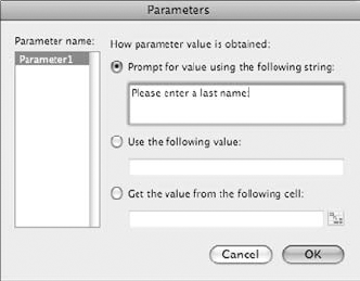

Figure 17.16. When you refresh data, you have the opportunity to enter a parameter value to pass to the query.
If all goes correctly, your list is refreshed with the data that matches the query. Figure 17.17 shows the results of our sample query. Now, every time you run the query, it plugs in the value of the parameter—from the cell, from the value you entered, or from a prompt.
Now that you've successfully imported data into a worksheet, it's time to remember why you wanted to do this in the first place: You want to take advantage of the power of Excel to work its number-crunching magic on it. One of the best ways this can be accomplished is through the use of PivotTables. A PivotTable is a special type of report that can help you analyze a set of data with contiguous values by letting you arrange it in a variety of ways. This section explains how you can build a PivotTable and illustrates with some examples. Figure 17.18 shows the data that we use for the examples.

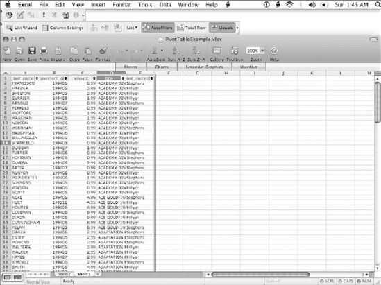
Figure 17.18. Here is the data that we have returned from a query to use as the basis for the PivotTable report. It includes customer, payment date, amount, movie title, and store manager information.
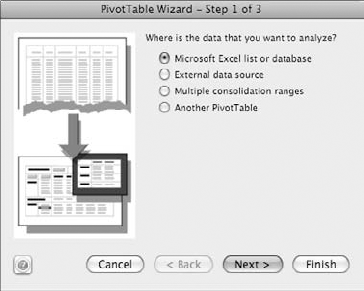
It's easy to build a PivotTable using the PivotTable Wizard. Perhaps the easiest way is to just get started. Suppose you want to create a table from a data range that you have imported into a worksheet. Follow these steps:
Select a cell in the data range that you want to use as the source of data for the PivotTable.
Choose Data
PivotTable Report.The PivotTable Wizard is launched, as shown in Figure 17.19.
In Step 1, select the first option for a data source: Microsoft Excel list or database.
You also can retrieve data directly from an external data source using Microsoft Query or choose multiple ranges to consolidate for the report. You can even use another PivotTable as a data source.
Click Next.
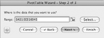
In Step 2 of the Wizard, shown in Figure 17.20, verify that Excel chose the correct data range that encompasses your selected cell. Make adjustments if necessary.
Click Next.
In Step 3, shown in Figure 17.21, you can choose to place the table in a new worksheet or an existing sheet. For this example, choose an existing sheet.
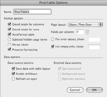
You can click the Options button to open the PivotTable Options dialog box, shown in Figure 17.22. In this dialog box, you can set various formatting and data options for the PivotTable.
You can click the Layout button to choose the cells to use for a preliminary layout. This layout can be changed later as you work with the table.
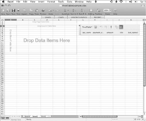
Click Finish to create the table. Figure 17.23 shows the blank PivotTable ready to have fields assigned to it.

In essence, a PivotTable is a multi-dimensional report that can be used to analyze multi-column data in various ways. To do that, you need to assign fields from the source data to the row, column, and data portions of the table, and let Excel do all the work to calculate totals based on the data.
When displaying a PivotTable, you first need to know which field you are ultimately interested in. In the case of our sample data, we want to get a sum of the payment totals for each movie title, so we drag the amount field to the data section. Because we want to tabulate payments per title, we can drag the title field to the rows section. Finally, we can drag the payment_date field to the columns section. By default, Excel automatically calculates a grand total for each title by summing the values for each month. It also calculates a grand total for each payment month, shown at the bottom of each column. This is shown in Figure 17.24.

Figure 17.24. By dragging and dropping different fields to the rows and columns, you can create PivotTable reports that show many different details from the same data. Here, we are generating a grand total for rental payments on each title.
Now, suppose we want to look at it differently and see how much each customer may have spent. We can replace the field used for the PivotTable rows with the last_name field, which is the last name of the customer. Figure 17.25 shows the new PivotTable.

Figure 17.25. By changing the field used for the PivotTable rows, we can generate a completely different table using the same data values.
Just to make it clear, let's try one more example. We'll keep the title in the rows spot and add last_name2, which is the name of the store manager. As Figure 17.26 shows, we can now see at a glance how much was spent on each title for each manager.
As you can see, PivotTable reports offer lots of options when it comes to viewing data.

So far you've seen much of what PivotTables can do, but we've barely scratched the surface. If you have looked closely, you have seen another section of the PivotTable report labeled "Drop Page Fields Here." This can be used to add yet another dimension to the PivotTable Report. If you drag one of your fields to this portion, you can filter your report to show items matching only a single value of that field. Figure 17.27 shows title versus payment date, but only for one manager.
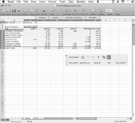
Figure 17.27. Using the Page field area, we can filter the data by a single value of that field. In this case, the table now shows sales for a single manager, Stephens.
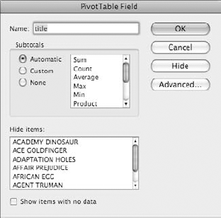
You can change these items:
Name: If you don't like the chosen name for a field, you can rename it to make your reports a little more readable. For example, we could change "last_name2" to "manager" to make it more clear what that field represents.
Subtotals: If the field is created from a calculation, you can change the function used to create it. The standard Excel functions of Sum, Count, Average, Max, Min, Product, and Count Nums can be used.
Hide Items: You can choose to hide certain fields, if you want to exclude them from the report.
Number: You can change the number format for fields that contain number values.
Hide: You can completely hide this field in the report.
Advanced: This launches the PivotTable Field Advanced Options dialog box, shown in Figure 17.29. In the Advanced dialog box, you can set AutoSort, AutoShow, and Page field data retrieval options.

When you're doing calculations, sometimes you know the result you are looking for, but you need to know what you have to do to achieve it. You can think of this as a reverse calculation, which can be handy for calculating loan terms and other financial calculations.
Excel's Goal Seek feature is designed to let you do that. Goal Seek works best when you already have data and formulas for your calculation in place and working correctly. Simply tell Excel which cell contains the formula, what the goal value is, and which cell contains the data value that you would like to change in order to meet your goal. Figure 17.30 contains an example of a worksheet with a formula in place to calculate an automobile loan.

Figure 17.30. Goal Seek is used with a working formula in place. It can vary one of the input values until the formula's result matches a goal value.
You can see in this example that cell C7 contains a formula for a loan payment:
=FMT(C6/12, C5, C4)
C6 contains the annual percentage rate (FMT requires a percentage rate based on the payment cycle, so it needs to be divided by 12 to get the monthly interest rate). C5 contains the term of the loan in months, and C4 contains the original amount of the loan. In this example, the monthly payment for a $30,000 loan for 60 months at an APR of 6.00% results in a monthly payment of $579.98.
Suppose we can only afford to pay $500 a month. In this case, we'd either need to lower the interest rate, increase the term, or decrease the loan amount. Goal Seek allows us to test any of these options.
To use Goal Seek for this example, follow these steps:
Select the cell that contains the formula. In this example, it's C7.
Choose Tools
Goal Seek. This opens the Goal Seek dialog box, shown in Figure 17.31. The Set cell should already reference the selected cell.Note
The Set cell always contains a formula or function.
Enter a value in the To value box. This is the desired result of the calculation.
Select one of the loan parameter cells as the Changing cell. The changing cell must always refer to a cell containing a value, not a formula or function.
Click OK. Excel attempts to calculate a proper value for the selected variable in order to have the formula result be the target value.

While it is calculating a goal, Excel displays the Goal Seek Status dialog box, shown in Figure 17.32. The Goal Seek Status dialog box shows you the calculations in progress. While Goal Seek runs, it iteratively substitutes new values into the Changing cell until it has run the calculation 100 times or has found an answer that is within .001 of the target value. (The maximum iterations and maximum change settings can be altered in the Calculations pane of the Excel Preferences dialog box.) If Goal Seek is unable to come up with a solution, the Step and Pause buttons become active, and you can use them to perform further iterations to try to reach your goal.

Excel can be a great tool for analyzing "what if" types of questions. You can use formulas and functions to create complex calculations, and then plug different data values into referenced cells to see how it changes the results. One problem with this is that you need to keep track of all the changes you make, and you may even need to save multiple versions of your workbook with different values in order to be able to go back to a particular calculation.
Excel 2008 offers a tool called the Scenario Manager to help you deal with these sorts of questions. You can use this tool to make changes to data values in a number of cells and save them under a unique scenario name, which can later be used to revisit or demonstrate how changes in values affect the calculations.
A scenario is simply the set of values that Excel can automatically plug into specified cells in your worksheets. This capability can be especially handy if you have a formula that calculates a result based on multiple input values. The following steps show how to use the Scenario Manager to create different scenarios:
Open the worksheet that you would like to run scenarios against.
Choose Tools
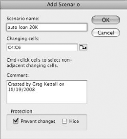
Scenarios to open the Scenario Manager dialog box, shown in Figure 17.33.Click Add to open the Add Scenario dialog box, which is shown in Figure 17.34.
Type a unique name for the scenario in the Scenario name box. Ideally, the name should provide some indication as to what conditions the scenario is testing.
Enter cell references for the cells to change in the Changing cells box. You can collapse down to the worksheet and select cells or to a range of cells. Use the

Choose protection options for the sheet. These take effect if you enable protection on the worksheet. Protection is explained in Chapter 12.
Prevent changes: This prevent users from making changes to the scenario if the worksheet is protected.
Hide: This hides the scenario from view if the worksheet is protected.
Click OK to open the Scenario Values dialog box, shown in Figure 17.35.
Enter the values that you want to use for this scenario for each selected cell.
If you want to create more scenarios, click Add and repeat Steps 4 through 8.
Click OK. All scenarios that you've created are now visible in the Scenario Manager.
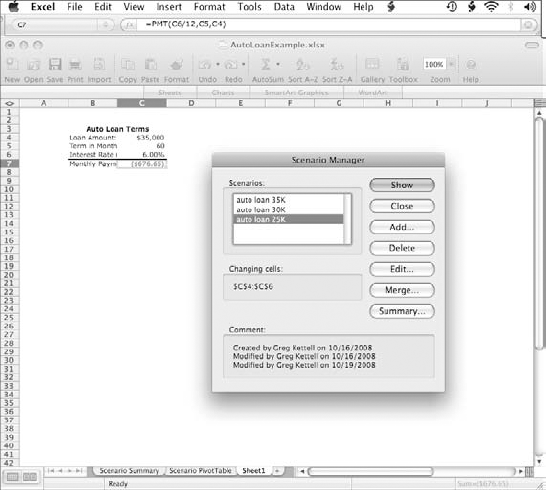

After you've created scenarios, you can test them using the Scenario Manager. Simply select the scenario you want to run, and click the Show button. The worksheet is updated with the saved values and the results recalculated. If you reach a scenario that you'd like to stick with, you can click the Close button to return to the worksheet. Alternatively, you can build a summary of all the scenarios, as explained later in this chapter.
Tip
To make your scenarios easier to understand at a glance, name your cells and use those names when entering changing cells. You can find more information about naming cells and ranges in Chapter 13.
Suppose you have workbooks with similar layouts (say, monthly or yearly reports), and you want to run the same scenarios in each of them. The Scenario Manager offers a merge capability that allows you to use scenarios created in one workbook in another. Note that this works only if the input cells are exactly the same between the two worksheets; otherwise, you must edit the imported scenarios. Follow these steps to merge scenarios from another workbook:
Open the workbook containing the original scenarios and the new one to which you want to add them.
In the new workbook, choose Tools
Scenarios to open the Scenario Manager.Click Merge to open the Merge Scenarios dialog box, shown in Figure 17.36.
Choose the workbook to import scenarios from the Book list.
If the workbook has multiple sheets, choose the sheet with the scenarios.
Click OK. The scenarios are added to the worksheet.

After you've created a few scenarios, it's nice to be able to see the effects of different data values all in one location. The Summary feature can be used to generate a new worksheet with either formatted data values or a PivotTable with the scenario values for further work. Follow these steps to create a scenario summary:
Open the Scenario Manager.
Click Summary.
Choose the option you want: Scenario Summary or Scenario PivotTable.
Enter the cell reference for the cell that contains the result of the calculation if it isn't correct.
Click OK. A new worksheet with either the Summary (shown in Figure 17.37) or PivotTable is created in the workbook.

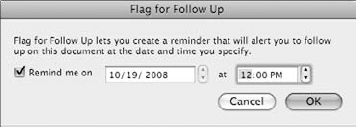
Sometimes when you are working with data, you may see something that catches your attention that you want to revisit at some point. You can flag your data for follow-up and get a notification to take a look. This can be helpful if you are working with data that you expect to be refreshed regularly. For example, you can set a follow-up notification for a time that is some point after the data has been modified so you'll be reminded to run a report. Another case where this could be useful is when you notice something amiss that you don't have time to deal with right away. Simply flag for follow-up, and you won't have to worry about it. To use this feature, choose Tools
The data form feature of Excel is intended to provide a quick and easy way to both manage and search for records in a list. If you have a row-column list with column headers, whether or not it uses the List Manager, do the following to use it in a data form:
Click any field in the list.
Choose Data
Form.The Data Form dialog box opens, as shown in Figure 17.39.
The dialog box is given a title that is the same as the worksheet from which it's launched.
To add new records to the list, click the New button or scroll to the end of the list, fill in the values in the fields, and click the New button again.
To search the list, click the Criteria button. Enter a value to search for in one of the data fields, and click the Find Next or Find Prev buttons.

Databases are ubiquitous in the corporate world, and being able to access and work efficiently with that data is a must. Excel's database connectivity capabilities using ODBC give it great flexibility in terms of the number and types of databases and data it can work with. All you need to get started is an ODBC driver for your particular database, and several third-party companies make drivers for the most popular database systems.
You learned how to create queries using the Microsoft Query tool and how to import that data into a worksheet. From there, it's a simple matter of utilizing the data, and one of the most powerful number-crunching tools Excel offers is the PivotTable report. This report can take data and present it in a myriad of ways, offering you tremendous flexibility in terms of finding out exactly what you want your data to tell you.
Finally, some additional Excel tools including Goal Seek and Scenarios were introduced, and you learned how to use them for "what-if" calculations. Finally, you saw yet another way to enter and search for data in your worksheets using the Data Form tool.