
4.6. Turbulent Reacting Flows and Turbulent Flames
Most practical combustion devices create flow conditions so that the fluid state of the fuel and oxidizer, or fuel–oxidizer mixture, is turbulent. Nearly all mobile and stationary power plants operate in this manner because turbulence increases the mass consumption rate of the reactants, or reactant mixture, to values much greater than those that can be obtained with laminar flames. A greater mass consumption rate increases the chemical energy release rate and hence the power available from a given combustor or internal engine of a given size. Indeed, few combustion engines could function without the increase in mass consumption during combustion that is brought about by turbulence. Another example of the importance of turbulence arises with respect to spark timing in automotive engines. As the RPM of the engine increases, the level of turbulence increases, whereupon the mass consumption rate (or turbulent flame speed) of the fuel–air mixture increases. This explains why spark timing does not have to be altered as the RPM of the engine changes with a given driving cycle.
As has been shown, the mass consumption rate per unit area in premixed laminar flames is simply ρSL, where ρ is the unburned gas mixture density. Correspondingly, for power plants operating under turbulent conditions, a similar consumption rate is specified as ρST, where ST is the turbulent burning velocity. Whether a well-defined turbulent burning velocity characteristic of a given combustible mixture exists as SL does under laminar conditions will be discussed later in this section. What is known is that the mass consumption rate of a given mixture varies with the state of turbulence created in the combustor. Explicit expressions for a turbulent burning velocity ST will be developed, and these expressions will show that various turbulent fields increase ST to values much larger than SL. However, increasing turbulence levels beyond a certain value increases ST little, if at all, and may lead to quenching of the flame [49].
To examine the effect of turbulence on flames, and hence the mass consumption rate of the fuel mixture, it is best to first recall the tacit assumption that in laminar flames the flow conditions alter neither the chemical mechanism nor the associated chemical energy release rate. Now one must acknowledge that in many flow configurations, there can be an interaction between the character of the flow and the reaction chemistry. When a flow becomes turbulent, there are fluctuating components of velocity, temperature, density, pressure, and concentration. The degree to which such components affect the chemical reactions, heat release rate, and flame structure in a combustion system depends upon the relative characteristic times associated with each of these individual parameters. In a general sense, if the characteristic time (τc) of the chemical reaction is much shorter than a characteristic time (τm) associated with the fluid-mechanical fluctuations, the chemistry is essentially unaffected by the flow field. But if the contra condition (τc > τm) is true, the fluid mechanics could influence the chemical reaction rate, energy release rates, and flame structure.
The interaction of turbulence and chemistry, which constitutes the field of turbulent reacting flows, is of importance whether flame structures exist or not. The concept of turbulent reacting flows encompasses many different meanings and depends on the interaction range, which is governed by the overall character of the flow environment. Associated with various flows are different characteristic times, or, as more commonly used, different characteristic lengths.
There are many different aspects to the field of turbulent reacting flows. Consider, for example, the effect of turbulence on the rate of an exothermic reaction typical of those occurring in a turbulent flow reactor. Here, the fluctuating temperatures and concentrations could affect the chemical reaction and heat release rates. Then, there is the situation in which combustion products are rapidly mixed with reactants in a time much shorter than the chemical reaction time. (This latter example is the so-called stirred reactor, which will be discussed in more detail in the next section.) In both of these examples, no flame structure is considered to exist.
Turbulence–chemistry interactions related to premixed flames comprise another major stability category. A turbulent flow field dominated by large-scale, low-intensity turbulence will affect a premixed laminar flame so that it appears as a wrinkled laminar flame. The flame would be contiguous throughout the front. As the intensity of turbulence increases, the contiguous flame front is partially destroyed and laminar flamelets exist within turbulent eddies. Finally, at very high-intensity turbulence, all laminar flame structure disappears and one has a distributed reaction zone. Time-averaged photographs of these three flames show a bushy flame front that looks thick in comparison to the smooth thin zone that characterizes a laminar flame. However, when a fast-response thermocouple is inserted into these three flames, the fluctuating temperatures in the first two cases show a bimodal probability density function with well-defined peaks at the temperatures of the unburned and completely burned gas mixtures, but a bimodal function is not found for the distributed reaction case.
Under premixed fuel–oxidizer conditions the turbulent flow field causes mixing between the different fluid elements, so the characteristic time was given the symbol τm. In general, with increasing turbulent intensity, this time approaches the chemical time, and the associated length approaches the flame or reaction zone thickness. Essentially the same is true with respect to non-premixed flames. The fuel and oxidizer (reactants) in non-premixed flames are not in the same flow stream; and since different streams can have different velocities, a gross shear effect can take place and coherent structures (eddies) can develop throughout this mixing layer. These eddies enhance the mixing of fuel and oxidizer. The same type of shear can occur under turbulent premixed conditions when large velocity gradients exist.
The complexity of the turbulent reacting flow problem is such that it is best to deal first with the effect of a turbulent field on an exothermic reaction in a plug flow reactor. Then the different turbulent reacting flow regimes will be described more precisely in terms of appropriate characteristic lengths, which will be developed from a general discussion of turbulence. Finally, the turbulent premixed flame will be examined in detail.
4.6.1. Rate of Reaction in a Turbulent Field
As an excellent, simple example of how fluctuating parameters can affect a reacting system, one can examine how the mean rate of a reaction would differ from the rate evaluated at the mean properties when there are no correlations among these properties. In flow reactors, time-averaged concentrations and temperatures are usually measured, and then rates are determined from these quantities. Only by optical techniques or fast-response thermocouples could the proper instantaneous rate values be measured, and these would fluctuate with time.
The fractional rate of change of a reactant can be written as
![]()
where the Yi's are the mass fractions of the reactants. The instantaneous change in rate is given by
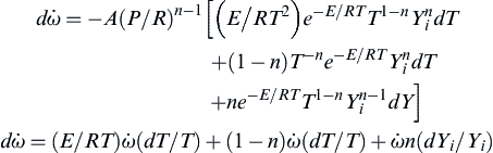
or
![]()
For most hydrocarbon flame or reacting systems the overall order of reaction is about 2, E/R is approximately 20,000 K, and the flame temperature is about 2000 K. Thus.
![]()
and it would appear that the temperature variation is the dominant factor. Since the temperature effect comes into this problem through the specific reaction rate constant, the problem simplifies to whether the mean rate constant can be represented by the rate constant evaluated at the mean temperature.
In this hypothetical simplified problem, one assumes further that the temperature T fluctuates with time around some mean represented by the form
![]()
where an is the amplitude of the fluctuation and f(t) is some time-varying function in which
![]()
and
over some time interval τ. T(t) can be considered to be composed of  , where T′ is the fluctuating component around the mean. Ignoring the temperature dependence in the pre-exponential, one writes the instantaneous-rate constant as
![]()
![]()
Dividing the two expressions, one obtains
![]()
Obviously, then, for small fluctuations
![]()
The expression for the mean rate is written as

But recall,
Examining the third term, it is apparent that

since the integral of the function can never be greater than 1. Thus,

If the amplitude of the temperature fluctuations is of the order of 10% of the mean temperature, one can take an ≈ 0.1; and if the fluctuations are considered sinusoidal, then

Thus for the example being discussed,

This result could be improved by assuming a more appropriate distribution function of T′ instead of a simple sinusoidal fluctuation; however, this example—even with its assumptions—usefully illustrates the problem. Normally, probability distribution functions are chosen. If the concentrations and temperatures are correlated, the rate expression becomes complicated. Bilger [50] presented a form of a two-component mean-reaction rate when it is expanded about the mean states, as follows:

4.6.2. Regimes of Turbulent Reacting Flows
The previous example epitomizes how the reacting media can be affected by a turbulent field. To understand the detailed effect, one must understand the elements of the field of turbulence. When considering turbulent combustion systems in this regard, a suitable starting point is the consideration of the quantities that determine the fluid characteristics of the system. The material presented subsequently has been mostly synthesized from Refs [51,52].
Most flows have at least one characteristic velocity, U, and one characteristic length scale, L, of the device in which the flow takes place. In addition there is at least one representative density ρ0 and one characteristic temperature T0, usually the unburned condition when considering combustion phenomena. Thus, a characteristic kinematic viscosity ν0 ≡ μ0/ρ0 can be defined, where μ0 is the coefficient of viscosity at the characteristic temperature T0. The Reynolds number for the system is then Re = UL/ν0. It is interesting that ν is approximately proportional to T2. Thus, an increase in temperature by a factor of three or more, modest by combustion standards, means a drop in Re by an order of magnitude. Thus, energy release can dampen turbulent fluctuations. The kinematic viscosity ν is inversely proportional to the pressure P, and changes in P are usually small; the effects of such changes in ν typically are much less than those due to changes in T.
Even though the Reynolds number gives some measure of turbulent phenomena, flow quantities characteristic of turbulence itself are of more direct relevance to modeling turbulent reacting systems. The turbulent kinetic energy  may be assigned a representative value
  at a suitable reference point. The relative intensity of the turbulence is then characterized by either
  or
or  , where
  is a representative root-mean-square velocity fluctuation. Weak turbulence corresponds to
  and intense turbulence has U′/U of the order unity.
Although a continuous distribution of length scales is associated with the turbulent fluctuations of velocity components and of state variables (P, ρ, T), it is useful to focus on two widely disparate lengths that determine separate effects in turbulent flows. First, there is a length l0, which characterizes the large eddies, those of low frequencies and long wavelengths; this length is sometimes referred to as the integral scale. Experimentally, l0 can be defined as a length beyond which various fluid-mechanical quantities become essentially uncorrelated; typically, l0 is less than L but of the same order of magnitude. This length can be used in conjunction with U′ to define a turbulent Reynolds number
![]()
which has more direct bearing on the structure of turbulence in flows than does Re. Large values of Rl can be achieved by intense turbulence, large-scale turbulence, and small values of ν produced, for example, by low temperatures or high pressures. The cascade view of turbulence dynamics is restricted to large values of Rl. From the characterization of U′ and l0, it is apparent that Rl < Re.
The second length scale characterizing turbulence is that over which molecular effects are significant; it can be introduced in terms of a representative rate of dissipation of velocity fluctuations, essentially the rate of dissipation of the turbulent kinetic energy. This rate of dissipation, which is given by the symbol ε0, is
This rate estimate corresponds to the idea that the time scale over which velocity fluctuations (turbulent kinetic energy) decay by a factor of (1/e) is the order of the turning time of a large eddy. The rate ε0 increases with turbulent kinetic energy (which is due principally to the large-scale turbulence) and decreases with increasing size of the large-scale eddies. For the small scales at which molecular dissipation occurs, the relevant parameters are the kinematic viscosity, which causes the dissipation, and the rate of dissipation. The only length scale that can be constructed from these two parameters is the so-called Kolmogorov length (scale):

However, note that
![]()
Therefore
![]()
This length is representative of the dimension at which dissipation occurs and defines a cut-off of the turbulence spectrum. For large Rl there is a large spread of the two extreme lengths characterizing turbulence. This spread is reduced with the increasing temperature found in combustion from the consequent increase in ν0.
Considerations analogous to those for velocity apply to scalar fields as well, and lengths analogous to lk have been introduced for these fields. They differ from lk by factors involving the Prandtl and Schmidt numbers, which differ relatively little from unity for representative gas mixtures. Therefore, to a first approximation for gases, lk may be used for all fields, and there is no need to introduce any new corresponding lengths.
An additional length, intermediate in size between l0 and lk, which often arises in formulations of equations for average quantities in turbulent flows is the Taylor length (λ), which is representative of the dimension over which strain occurs in a particular viscous medium. The strain can be written as (U′/l0). As before, the length that can be constructed between the strain and the viscous forces is
![]()
![]()
and then
![]()
In a sense, the Taylor microscale is similar to an average of the other scales, l0 and lk, but heavily weighted toward lk.
Recall that there are length scales associated with laminar flame structures in reacting flows. One is the characteristic thickness of a premixed flame, δL, given by
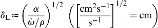
The derivation is, of course, consistent with the characteristic velocity in the flame speed problem. This velocity is obviously the laminar flame speed itself, so that
![]()
As discussed in an earlier section, δL is the characteristic length of the flame and includes the thermal preheat region and that associated with the zone of rapid chemical reaction. This reaction zone is the rapid heat release flame segment at the high-temperature end of the flame. The earlier discussion of flame structure from detailed chemical kinetic mechanisms revealed that the heat release zone need not be narrow compared with the preheat zone. Nevertheless, the magnitude of δL does not change, no matter what the analysis of the flame structure is. It is then possible to specify the characteristic time of the chemical reaction in this context to be
![]()
It may be expected, then, that the nature of the various turbulent flows, and indeed the structures of turbulent flames, may differ considerably and their characterization would depend on the comparison of these chemical and flow scales in a manner specified by the following inequalities and designated flame type:

The nature, or more precisely the structure, of a particular turbulent flame implied by these inequalities cannot be exactly established at this time. The reason is that values of δL, lk, λ, or l0 cannot be explicitly measured under a given flow condition or analytically estimated. Many of the early experiments with turbulent flames appear to have operated under the condition δL < lk, so the early theories that developed specified this condition in expressions for ST. The flow conditions under which δL would indeed be less than lk have been explored analytically in detail and will be discussed subsequently.
To expand on the understanding of the physical nature of turbulent flames, it is also beneficial to look closely at the problem from a chemical point of view, exploring how heat release and its rate affect turbulent flame structure.
One begins with the characteristic time for chemical reaction designated τc, which was defined earlier. (Note that this time would be appropriate whether a flame existed or not.) Generally, in considering turbulent reacting flows, chemical lengths are constructed to be Uτc or U′τc. Then comparison of an appropriate chemical length with a fluid dynamic length provides a nondimensional parameter that has a bearing on the relative rate of reaction. Nondimensional numbers of this type are called Damkohler numbers and are conventionally given the symbol Da. An example appropriate to the considerations here is
![]()
where τm is a mixing (turbulent) time defined as (l0/U′), and the last equality in the expression applies when there is a flame structure. Following the earlier development, it is also appropriate to define another turbulent time based on the Kolmogorov scale τk = (ν/ε0)1/2.
For large Damkohler numbers, the chemistry is fast (i.e., reaction time is short) and reaction sheets of various wrinkled types may occur. For small Da numbers, the chemistry is slow and well-stirred flames may occur.
Two other nondimensional numbers relevant to the chemical reaction aspect of this problem [51] were introduced by Frank–Kamenetskii and others. These Frank–Kamenetskii numbers (FK) are the nondimensional heat release FK1 ≡ (Qp/cpTf), where Qp is the chemical heat release of the mixture and Tf is the flame (or reaction) temperature; and the nondimensional activation energy FK2 ≡ (Ta/Tf), where the activation temperature Ta = (EA/R). Combustion, in general, and turbulent combustion, in particular, are typically characterized by large values of these numbers. When FK1 is large, chemistry is likely to have a large influence on turbulence. When FK2 is large, the rate of reaction depends strongly on the temperature. It is usually true that the larger the FK2, the thinner will be the region in which the principal chemistry occurs. Thus, irrespective of the value of the Damkohler number, reaction zones tend to be found in thin, convoluted sheets in turbulent flows, for both premixed and non-premixed systems having large FK2. For premixed flames, the thickness of the reaction region has been shown to be of the order δL/FK2. Different relative sizes of δL/FK2 and fluid-mechanical lengths, therefore, may introduce additional classes of turbulent reacting flows.
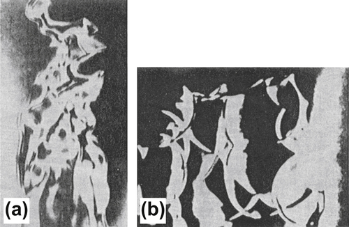
The flames themselves can alter the turbulence. In simple open Bunsen flames whose tube Reynolds number indicates that the flow is in the turbulent regime, some results have shown that the temperature effects on the viscosity are such that the resulting flame structure is completely laminar. Similarly, for a completely laminar flow in which a simple wire is oscillated near the flame surface, a wrinkled flame can be obtained (Figure 4.41). Certainly, this example is relevant to δL < lk; that is, a wrinkled flame. Nevertheless, most open flames created by a turbulent fuel jet exhibit a wrinkled flame type of structure. Indeed, short-duration Schlieren photographs suggest that these flames have continuous surfaces. Measurements of flames such as that shown in Figures. 4.42(a) and (b) have been taken at different time intervals, and the instantaneous flame shapes verify the continuous wrinkled flame structure. A plot of these instantaneous surface measurements results in a thick flame region (Figure 4.43), just as the eye would visualize that a larger number of these measurements would result in a thick flame. Indeed, turbulent premixed flames are described as bushy flames. The thickness of this turbulent flame zone appears to be related to the scale of turbulence. Essentially, this case becomes that of severe wrinkling and is categorized by lk < δL < λ. Increased turbulence changes the character of the flame wrinkling, and flamelets begin to form. These flame elements take on the character of a fluid-mechanical vortex rather than a simple distorted wrinkled front, and this case is specified by λ < δL < l0. For δL << l0, some of the flamelets fragment from the front, and the flame zone becomes highly wrinkled with pockets of combustion. To this point, the flame is considered practically contiguous. When l0 < δL, contiguous flames no longer exist, and a distributed reaction front forms. Under these conditions, the fluid mixing processes are rapid with respect to the chemical reaction time, and the reaction zone essentially approaches the condition of a stirred reactor. In such a reaction zone, products and reactants are continuously intermixed.

For a better understanding of this type of flame occurrence and for more explicit conditions that define each of these turbulent flame types, it is necessary to introduce the flame stretch concept. This will be done shortly, at which time the regions will be more clearly defined with respect to chemical and flow rates with a graph that relates the nondimensional turbulent intensity, Reynolds numbers, Damkohler number, and characteristic lengths l.
First, however, consider that in turbulent Bunsen flames the axial component of the mean velocity along the centerline remains almost constant with height above the burner; but away from the centerline, the axial mean velocity increases with height. The radial outflow component increases with distance from the centerline and reaches a peak outside the flame. Both axial and radial components of turbulent velocity fluctuations show a complex variation with position and include peaks and troughs in the flame zone. Thus, there are indications of both generation and removal of turbulence within the flame. With increasing height above the burner, the Reynolds shear stress decays from that corresponding to an initial pipe flow profile.

In all flames there is a large increase in velocity as the gases enter the burned gas state. Thus, it should not be surprising that the heat release itself can play a role in inducing turbulence. Such velocity changes in a fixed combustion configuration can cause shear effects that contribute to the turbulence phenomenon. There is no better example of some of these aspects than the case in which turbulent flames are stabilized in ducted systems. The mean axial velocity field of ducted flames involves considerable acceleration resulting from gas expansion engendered by heat release. Typically, the axial velocity of the unburned gas doubles before it is entrained into the flame, and the velocity at the centerline at least doubles again. Large mean velocity gradients are therefore produced. The streamlines in the unburned gas are deflected away from the flame.
The growth of axial turbulence in the flame zone of these ducted systems is attributed to the mean velocity gradient resulting from the combustion. The production of turbulence energy by shear depends on the product of the mean velocity gradient and the Reynolds stress. Such stresses provide the most plausible mechanism for the modest growth in turbulence observed.
Now it is important to stress that whereas the laminar flame speed is a unique thermochemical property of a fuel–oxidizer mixture ratio, a turbulent flame speed is a function not only of the fuel–oxidizer mixture ratio but also of the flow characteristics and experimental configuration. Thus, one encounters great difficulty in correlating the experimental data of various investigators. In a sense, there is no flame speed in a turbulent stream. Essentially, as a flow field is made turbulent for a given experimental configuration, the mass consumption rate (and hence the rate of energy release) of the fuel–oxidizer mixture increases. Therefore, some researchers have found it convenient to define a turbulent flame speed ST as the mean mass flux per unit area (in a coordinate system fixed to the time-averaged motion of the flame) divided by the unburned gas density ρ0. The area chosen is the smoothed surface of the time-averaged flame zone. However, this zone is thick and curved; thus, the choice of an area near the unburned gas edge can give a different result from one in which a flame position is taken in the center or the burned-gas side of the bushy flame. Therefore, a great deal of uncertainty is associated with the various experimental values of ST reported. Nevertheless, definite trends have been reported. These trends can be summarized as follows:
1. ST is always greater than SL. This trend would be expected once the increased area of the turbulent flame allows greater total mass consumption.
2. ST increases with increasing intensity of turbulence ahead of the flame. Many have found the relationship to be approximately linear. (This point will be discussed later.)
3. Some experiments show ST to be insensitive to the scale of the approach flow turbulence.
4. In open flames, the variation of ST with composition is generally much the same as for SL, and ST has a well-defined maximum close to stoichiometric. Thus, many report turbulent flame speed data as the ratio of ST/SL.
5. Very large values of ST may be observed in ducted burners at high approach flow velocities. Under these conditions, ST increases in proportion to the approach flow velocities but is insensitive to approach flow turbulence and composition. It is believed that these effects result from the dominant influence of turbulence generated within the stabilized flame by the large velocity gradients.
The definition of the flame speed as the mass flux through the flame per unit area of the flame divided by the unburned gas density ρ0 is useful for turbulent nonstationary and oblique flames as well.
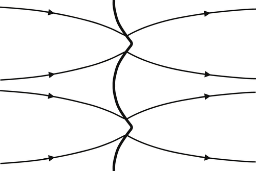
Now with regard to stretch, consider first a plane oblique flame. Because of the increase in velocity demanded by continuity, a streamline through such an oblique flame is deflected toward the direction of the normal to the flame surface. The velocity vector may be broken up into a component normal to the flame wave and a component tangential to the wave (Figure 4.44). Because of the energy release, the continuity of mass requires that the normal component increase on the burned gas side while, of course, the tangential component remains the same. A consequence of the tangential velocity is that fluid elements in the oblique flame surface move along this surface. If the surface is curved, adjacent points traveling along the flame surface may move either farther apart (flame stretch) or closer together (flame compression).

An oblique flame is curved if the velocity U of the approach flow varies in a direction y perpendicular to the direction of the approach flow. Strehlow showed that the quantity
![]()
which is known as the Karlovitz flame stretch factor, is approximately equal to the ratio of the flame thickness δL to the flame curvature. The Karlovitz school has argued that excessive stretching can lead to local quenching of the reaction. Klimov [53], and later Williams [54], analyzed the propagation of a laminar flame in a shear flow with velocity gradient in terms of a more general stretch factor
![]()
where Λ is the area of an element of flame surface, dΛ/dt is its rate of increase, and δL/SL is a measure of the transit time of the gases passing through the flame. Stretch (K2 > 0) is found to reduce the flame thickness and to increase reactant consumption per unit area of the flame and large stretch (K2 >> 0) may lead to extinction. On the other hand, compression (K2 < 0) increases flame thickness and reduces reactant consumption per unit incoming reactant area. These findings are relevant to laminar flamelets in a turbulent flame structure.
Since the concern here is with the destruction of a contiguous laminar flame in a turbulent field, consideration must also be given to certain inherent instabilities in laminar flames themselves. There is a fundamental hydrodynamic instability as well as an instability arising from the fact that mass and heat can diffuse at different rates; that is, the Lewis number (Le) is nonunity. In the latter mechanism, a flame instability can occur when the Le number (α/D) is less than 1.
Consider initially the hydrodynamic instability—that is, the one due to the flow—first described by Darrieus [55], Landau [56], and Markstein [57]. If no wrinkle occurs in a laminar flame, the flame speed SL is equal to the upstream unburned gas velocity U0. But if a minor wrinkle occurs in a laminar flame, the approach flow streamlines will either diverge or converge, as shown in Figure 4.45. Considering the two middle streamlines, one notes that because of the curvature owing to the wrinkle, the normal component of the velocity with respect to the flame is less than U0. Thus, the streamlines diverge as they enter the wrinkled flame front. Since there must be continuity of mass between the streamlines, the unburned gas velocity at the front must decrease owing to the increase of area. Since SL is now greater than the velocity of unburned approaching gas, the flame moves farther downstream and the wrinkle is accentuated. For similar reasons, between another pair of streamlines if the unburned gas velocity increases near the flame front, the flame bows in the upstream direction. It is not clear why these instabilities do not keep growing. Some have attributed the growth limit to nonlinear effects that arise in hydrodynamics.
When the Lewis number is nonunity, the mass diffusivity can be greater than the thermal diffusivity. This discrepancy in diffusivities is important with respect to the reactant that limits the reaction. Ignoring the hydrodynamic instability, consider again the condition between a pair of streamlines entering a wrinkle in a laminar flame. This time, however, look more closely at the flame structure that these streamlines encompass, noting that the limiting reactant will diffuse into the flame zone faster than heat can diffuse from the flame zone into the unburned mixture. Thus, the flame temperature rises, the flame speed increases, and the flame wrinkles bow further in the downstream direction. The result is a flame that looks much like the flame depicted for the hydrodynamic instability in Figure 4.45. The flame surface breaks up continuously into new cells in a chaotic manner, as photographed by Markstein [54]. There appears to be, however, a higher-order stabilizing effect. The fact that the phenomenon is controlled by a limiting reactant means that this cellular condition can occur when the unburned premixed gas mixture is either fuel-rich or fuel-lean. It should not be surprising, then, that the most susceptible mixture would be a lean hydrogen–air system.
Earlier it was stated that the structure of a turbulent velocity field may be presented in terms of two parameters—the scale and the intensity of turbulence. The intensity was defined as the square root of the turbulent kinetic energy, which essentially gives a root-mean-square velocity fluctuation U′. Three length scales were defined: the integral scale l0, which characterizes the large eddies; the Taylor microscale λ, which is obtained from the rate of strain; and the Kolmogorov microscale lk, which typifies the smallest dissipative eddies. These length scales and the intensity can be combined to form not one, but three turbulent Reynolds numbers: Rl = U′l0/ν, Rλ = U′λ/ν, and Rk = U′lk/ν. From the relationship between l0, λ, and lk previously derived it is found that  .
.
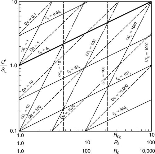
There is now sufficient information to relate the Damkohler number Da and the length ratios l0/δL, lk/δL and l0/lk to a nondimensional velocity ratio U′/SL and the three turbulence Reynolds numbers. The complex relationships are given in Figure 4.46 and are informative. The right-hand side of the figure has Rλ > 100 and ensures the length-scale separation that is characteristic of high Reynolds number behavior. The largest Damkohler numbers are found in the bottom right corner of the figure.
Using this graph and the relationship it contains, one can now address the question of whether and under what conditions a laminar flame can exist in a turbulent flow. As before, if allowance is made for flame front curvature effects, a laminar flame can be considered stable to a disturbance of sufficiently short wavelength; however, intense shear can lead to extinction. From solutions of the laminar flame equations in an imposed shear flow, Klimov [53] and Williams [54] showed that a conventional propagating flame may exist only if the stretch factor K2 is less than a critical value of unity. Modeling the area change term in the stretch expression as
![]()
and recalling that
![]()
one can define the Karlovitz number for stretch in turbulent flames as
![]()
with no possibility of negative stretch. Thus,

But as shown earlier
![]()
so that
![]()
Thus, the criterion to be satisfied if a laminar flame is to exist in a turbulent flow is that the laminar flame thickness δL be less than the Kolmogorov microscale lk of the turbulence.
The heavy line in Figure 4.46 indicates the conditions δL = lk. This line is drawn in this fashion since

Thus, for (U′/SL) = 1, Rλ = 1; and for (U′/SL) = 10, Rλ = 100. The other Reynolds numbers follow from  .
.
Below and to the right of this line, the Klimov–Williams criterion is satisfied and wrinkled laminar flames may occur. The figure shows that this region includes both large and small values of turbulence Reynolds numbers and velocity ratios (U′/SL) both greater and less than 1, but predominantly large Da.
Above and to the left of the criterion line is the region in which lk < δL. According to the Klimov–Williams criterion, the turbulent velocity gradients in this region, or perhaps in a region defined with respect to any of the characteristic lengths, are sufficiently intense that they may destroy a laminar flame. The figure shows U′ ≥ SL in this region and Da is predominantly small. At the highest Reynolds numbers the region is entered only for intense turbulence, U′ > SL. The region has been considered a distributed reaction zone in which reactants and products are somewhat uniformly dispersed throughout the flame front. Reactions are still fast everywhere, so that unburned mixture near the burned-gas side of the flame is completely burned before it leaves what would be considered the flame front. An instantaneous temperature measurement in this flame would yield a normal probability density function—more important, one that is not bimodal.
4.6.3. Turbulent Flame Speed
Although a laminar flame speed SL is a physicochemical and chemical kinetic property of the unburned gas mixture that can be assigned, a turbulent flame speed ST is in reality a mass consumption rate per unit area divided by the unburned gas mixture density. Thus, ST must depend on the properties of the turbulent field in which it exists and the method by which the flame is stabilized. Of course, difficulty arises with this definition of ST because the time-averaged turbulent flame is bushy (thick), and there is a large difference between the area on the unburned-gas side of the flame and that on the burned-gas side. Nevertheless, many experimental data points are reported as ST.
In his attempts to analyze the early experimental data, Damkohler [58] considered that large-scale, low-intensity turbulence simply distorts the laminar flame while the transport properties remain the same; thus, the laminar flame structure would not be affected. Essentially, his concept covered the range of the wrinkled and severely wrinkled flame cases defined earlier. Whereas a planar laminar flame would appear as a simple Bunsen cone, that cone is distorted by turbulence as shown in Figure 4.43. It is apparent, then, that the area of the laminar flame will increase owing to a turbulent field. Thus, Damkohler [58] proposed for large-scale, small-intensity turbulence that
![]()
where AL is the total area of laminar surface contained within an area of turbulent flame whose time-averaged area is AT. Damkohler further proposed that the area ratio could be approximated by
![]()
which leads to the results
![]()
where  is the turbulent intensity of the unburned gases ahead of the turbulent flame front.
Many groups of experimental data have been evaluated by semiempirical correlations of the type
![]()
![]()
The first expression here is similar to the Damkohler result for A and B equal to 1. Since the turbulent exchange coefficient (eddy diffusivity) correlates well with l0U′ for tube flow, and indeed, l0 is essentially constant for the tube flow characteristically used for turbulent premixed flame studies, it follows that
![]()
where Re is the tube Reynolds number. Thus, the latter expression has the same form as the Damkohler result except that the constants would have to equal 1 and SL, respectively, for similarity.
Schelkin [59] also considered large-scale, small-intensity turbulence. He assumed that flame surfaces distort into cones with bases proportional to the square of the average eddy diameter (i.e., proportional to l0). The height of the cone was assumed proportional to U′ and to the time t during which an element of the wave is associated with an eddy. Thus, time can be taken as equal to (l0/SL). Schelkin then proposed that the ratio of ST/SL (average) equals the ratio of the average cone area to the cone base. From the geometry thus defined,
![]()
where AC is the surface area of the cone and AB is the area of the base. Therefore,
![]()
For large values of  , that is, high-intensity turbulence, the preceding expression reduces to that developed by Damkohler:
  .
.
A more rigorous development of wrinkled turbulent flames led Clavin and Williams [60] to the following result where isotropic turbulence is assumed:

This result differs from Schelkin's heuristic approach only by the factor of two in the second term. The Clavin-Williams expression is essentially restricted to the case of  . For small , the Clavin-Williams expression simplifies to
![]()
which is similar to the Damkohler result. Kerstein and Ashurst [61], in a reinterpretation of the physical picture of Clavin and Williams, proposed the expression
![]()
Using a direct numerical simulation, Yakhot [62] proposed the relation
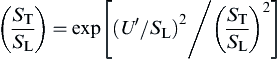
For small-scale, high-intensity turbulence, Damkohler reasoned that the transport properties of the flame are altered from laminar kinetic theory viscosity ν0 to the turbulent exchange coefficient ε so that
![]()
This expression derives from SL ∼ α1/2 ∼ ν1/2. Then, realizing that  ,
,
![]()
Schelkin [59] also extended Damkohler's model by starting from the fact that the transport in a turbulent flame could be made up of molecular movements (laminar λL) and turbulent movements, so that
![]()
where the expression is again analogous to that for SL. (Note that λ is the thermal conductivity in this equation, not the Taylor scale.) Then it would follow that
![]()
and
![]()
or essentially
![]()
The Damkohler turbulent exchange coefficient ε is the same as νT, so that both expressions are similar, particularly in that for high-intensity turbulence ε >> ν. The Damkohler result for small-scale, high-intensity turbulence that
![]()
is significant, for it reveals that (ST/SL) is independent of  at fixed Re. Thus, as stated earlier, increasing turbulence levels beyond a certain value increases ST little, if at all. In this regard, it is well to note that Ronney [39] reported “smoothed” experimental data from Bradley [49] in the form (ST/SL) versus for Re = 1000. Ronney’s correlations of these data are reinterpreted in Figure 4.47. Recall that all the expressions for small-intensity, large-scale turbulence were developed for small values of and reported a linear relationship between and (ST/SL). It is not surprising, then, that a plot of these expressions—and even some more advanced efforts that also show linear relations—do not correlate well with the curve in Figure 4.47. Furthermore, most developments do not take into account the effect of stretch on the turbulent flame. Indeed, the expressions reported here hold and show reasonable agreement with experiment only for
  . Bradley [49] suggested that burning velocity is reduced with stretch—that is, as the Karlovitz stretch factor K2 increases. There are also some Lewis number effects. Refer to Ref. [39] for more details and further insights.


The general data representation in Figure 4.47 shows a rapid rise of (ST/SL) for values of . It is apparent from the discussion to this point that as becomes greater than 1, the character of the turbulent flame varies; and under the appropriate turbulent variables, it can change as depicted in Figure 4.48, which essentially comes from Borghi [63] as presented by Abdel-Gayed et al. [64].
..................Content has been hidden....................
You can't read the all page of ebook, please click here login for view all page.