Chapter 1 discusses basic chemical thermodynamics and flame temperatures for combustion analysis. Heats of reaction, free energy, and equilibrium constants are introduced and then applied for the analysis of chemical equilibrium composition and adiabatic flame temperature of fuel−oxidizer mixtures. The effects of mixture equivalence ratio and pressure on the flame temperature and composition are discussed along with practical considerations. A brief discussion of sub and supersonic combustion thermodynamics is also presented.
Keywords
Chemical thermodynamics; Equilibrium constants; Flame temperatures; Free energy; Heats of reaction
1.1. Introduction
The parameters essential for the evaluation of combustion systems are the equilibrium product temperature and composition. If all the heat evolved in the reaction is employed solely to raise the product temperature, this temperature is called the adiabatic flame temperature. Because of the importance of the temperature and gas composition in combustion considerations, it is appropriate to review those aspects of the field of chemical thermodynamics that deal with these subjects.
1.2. Heats of Reaction and Formation
All chemical reactions are accompanied either by an absorption or evolution of energy, which usually manifests itself as heat. It is possible to determine this amount of heat—and hence the temperature and product composition—from very basic principles. Spectroscopic data and statistical calculations permit one to determine the internal energy of a substance. The internal energy of a given substance is found to be dependent upon its temperature, pressure, and state and is independent of the means by which the state is attained. Likewise the change in internal energy, ΔE, of a system that results from any physical change or chemical reaction depends only on the initial and final state of the system. Regardless of whether the energy is evolved as heat or work, the total change in internal energy will be the same.
If a flow reaction proceeds with negligible changes in kinetic energy and potential energy and involves no form of work beyond that required for the flow, the heat added is equal to the increase of enthalpy of the system
Q=ΔH
where Q is the heat added and H is the enthalpy. For a nonflow reaction proceeding at constant pressure, the heat added is also equal to the gain in enthalpy
Qp=ΔH
and if heat is evolved,
Qp=−ΔH
Most thermochemical calculations are made for closed thermodynamic systems, and the stoichiometry is most conveniently represented in terms of the molar quantities. In dealing with compressible flow problems in which it is essential to work with open thermodynamic systems, it is best to employ mass quantities. Throughout this text uppercase symbols will be used for molar quantities and lowercase symbols for mass quantities.
One of the most important thermodynamic facts to know about a given chemical reaction is the change in energy or heat content associated with the reaction at some specified temperature, where each of the reactants and products is in an appropriate standard state. This change is known either as the enthalpy of reaction or as the heat of reaction at the specified temperature.
The standard state means that for each state a reference state of the aggregate exists. For gases, the thermodynamic standard reference state is the ideal gaseous state at atmospheric pressure at each temperature. The ideal gaseous state is the case of isolated molecules which give no interactions and which obey the equation of state of a perfect gas. The standard reference state for pure liquids and solids at a given temperature is the real state of the substance at a pressure of 1 atm. As discussed in Chapter 9, understanding this definition of the standard reference state is very important when considering the case of high-temperature combustion in which the product composition contains a substantial mole fraction of a condensed phase, such as a metal oxide.
The thermodynamic symbol that represents the property of the substance in the standard state at a given temperature is written, for example, as H°T,E°T, etc., where the ‘degree sign’ superscript ° specifies the standard state and the subscript T, the specific temperature. Statistical mechanics calculations actually permit the determination of ET−E0, which is the energy content at a given temperature referenced to the energy content at 0 K. For one mole in the ideal gaseous state
PV=RT
(1.1)
H°=E°+(PV)°=E°+RT
(1.2)
which at 0 K reduces to
H°0=E°0
(1.3)
Thus the heat content at any temperature referred to the heat or energy content at 0 K is known and
(H°−H°0)=(E°−E°0)+RT=(E°−E°0)+PV
(1.4)
The value (E°−E°0) is determined from spectroscopic information and is actually the energy in the internal (rotational, vibrational, and electronic) and external (translational) degrees of freedom of the molecule. Enthalpy (H°−H°0) has meaning only when there is a group of molecules, a mole for instance; it is thus the ability of a group of molecules with internal energy to do PV work. In this sense, then, a single molecule can have internal energy, but not enthalpy. As stated, the use of the lowercase symbol will signify values on a mass basis. Since flame temperatures are calculated for a closed thermodynamic system of fixed mass, and molar conservation is not required, working on a molar basis is most convenient. In flame propagation or reacting flows through nozzles, mass is conserved as it crosses system boundaries; thus when these systems are considered, the per-unit mass basis of the thermochemical properties is used for a convenient solution.
Figure 1.1Heats of reactions at different base temperatures.
From the definition of the heat of reaction, Qp will depend on the temperature T at which the reaction and product enthalpies are evaluated. The heat of reaction at one temperature T0 can be related to that at another temperature T1. Consider the reaction configuration shown in Figure 1.1. According to the First Law of Thermodynamics, the changes in energy that proceed from reactants at temperature T0 to products at temperature T1, by either path A or path B must be the same. Path A raises the reactants from temperature T0 to T1, and reacts at T1. Path B reacts at T0 and raises the products from T0 to T1. This energy equality, which relates the heats of reaction at the two different temperatures, is written as
where n specifies the number of moles of the ith product or jth reactant. Any phase changes can be included in the heat content terms. Thus, by knowing the difference in energy content at the different temperatures for the products and reactants, it is possible to determine the heat of reaction at one temperature from the heat of reaction at another.
If the heats of reaction at a given temperature are known for two separate reactions, the heat of reaction of a third reaction at the same temperature may be determined by simple algebraic addition. This statement is the Law of Heat Summation. For example, reactions (1.6) and (1.7) can be carried out conveniently in a calorimeter at constant pressure:
Cgraphite+O2(g)→298KCO2(g),Qp=+393.52kJ
(1.6)
CO(g)+12O2(g)→298KCO2(g),Qp=+283.0kJ
(1.7)
Subtracting these two reactions, one obtains
Cgraphite+12O2(g)→298KCO(g),Qp=+110.52kJ
(1.8)
Since some of the carbon would burn to CO2 and not solely to CO, it is difficult to determine calorimetrically the heat released by reaction (1.8).
It is, of course, not necessary to have an extensive list of heats of reaction to determine the heat absorbed or evolved in every possible chemical reaction. A more convenient and logical procedure is to list the standard heats of formation of chemical substances. The standard heat of formation is the enthalpy of a substance in its standard state referred to its elements in their standard states at the same temperature. From this definition it is obvious that heats of formation of the elements in their standard states are zero.
The value of the heat of formation of a given substance from its elements may be the result of the determination of the heat of one reaction. Thus, from the calorimetric reaction for burning carbon to CO2 (Eqn (1.6)), it is possible to write the heat of formation of carbon dioxide at 298 K as
(ΔH°f)298,CO2=−393.52kJ/mol
The superscript to the heat of formation symbol ΔH°f represents the standard state, and the subscript number represents the base or reference temperature. From the example for the Law of Heat Summation, it is apparent that the heat of formation of carbon monoxide from Eqn (1.8) is
(ΔH°f)298,CO=−110.52kJ/mol
It is evident that, by judicious choice, the number of reactions that must be measured calorimetrically will be about the same as the number of substances whose heats of formation are to be determined.
The logical consequence of the preceding discussion is that, given the heats of formation of the substances comprising any particular reaction, one can directly determine the heat of reaction or heat evolved at the reference temperature T0, most generally T298, as follows:
ΔHT0=∑iprodni(ΔH°f)T0,i−∑jreactnj(ΔH°f)T0,j=−Qp
(1.9)
Extensive tables of standard heats of formation are available, but they are not all at the same reference temperature. The most convenient are the compilations known as the JANAF [1] and NBS Tables [2], both of which use 298 K as the reference temperature and are now available as the NIST-JANAF Thermochemical Tables (http://kinetics.nist.gov/janaf/). Table 1.1 lists some values of the heat of formation taken from the JANAF Thermochemical Tables. Actual JANAF tables are reproduced in Appendix A. These tables, which represent only a small selection from the JANAF volume, were chosen as those commonly used in combustion and to aid in solving the problem sets throughout this book. Note that, although the developments throughout this book take the reference state as 298 K, the JANAF Tables also list ΔH°f for all temperatures.
When the products are measured at a temperature T2 different from the reference temperature T0, and the reactants enter the reaction system at a temperature T′0 different from the reference temperature, the heat of reaction becomes
The reactants in most systems are considered to enter at the standard reference temperature 298 K. Consequently, the enthalpy terms in the braces for the reactants disappear. The JANAF Tables tabulate, as a putative convenience, (H°T−H°298) instead of (H°T−H°0). This type of tabulation is unfortunate since the reactants for systems using cryogenic fuels and oxidizers, such as those used in rockets, can enter the system at temperatures lower than the reference temperature. Indeed, the fuel and oxidizer individually could enter at different temperatures. Thus the summation in Eqn (1.10) is handled most conveniently by realizing that T′0 may vary with the substance j.
The values of heats of formation reported in Table 1.1 are ordered so that the largest positive values of the heats of formation per mole are the highest, and those with negative heats of formation are the lowest. In fact, this table is similar to a potential energy chart. As species at the top react to form species at the bottom, heat is released, and an exothermic system exists. Even a species that has a negative heat of formation can react to form products of still lower negative heats of formation species, thereby releasing heat. Since some fuels that have negative heats of formation form many moles of product species having negative heats of formation, the heat release in such cases can be large. Equation (1.9) shows this result clearly. Indeed, the first summation in Eqn (1.9) is generally much greater than the second. Thus the characteristic of the reacting species or the fuel that significantly determines the heat release is its chemical composition and not necessarily its molar heat of formation. As explained in Section 1.4.2, the heats of formation listed on a per unit mass basis simplifies one's ability to estimate the relative heat release and flame temperature of one fuel to another without the detailed calculations reported later in this chapter and in Appendix I.
Table 1.1
Heats of Formation at 298 K
Chemical
Name
State
ΔH∘f(kJ/mol)
Δh∘f(kJ/g)
C
Carbon
Vapor
716.67
59.72
N
Nitrogen atom
Gas
472.68
33.76
O
Oxygen atom
Gas
249.17
15.57
C2H2
Acetylene
Gas
226.73
8.72
H
Hydrogen atom
Gas
218.00
218.00
O3
Ozone
Gas
142.67
2.97
NO
Nitric oxide
Gas
90.29
3.01
C6H6
Benzene
Gas
82.96
1.06
C6H6
Benzene
Liquid
49.06
0.63
C2H4
Ethene
Gas
52.38
1.87
N2H4
Hydrazine
Liquid
50.63
1.58
OH
Hydroxyl radical
Gas
38.99
2.29
O2
Oxygen
Gas
0
0
N2
Nitrogen
Gas
0
0
H2
Hydrogen
Gas
0
0
C
Carbon
Solid
0
0
NH3
Ammonia
Gas
−45.90
−2.70
C2H4O
Ethylene oxide
Gas
−51.08
−0.86
CH4
Methane
Gas
−74.87
−4.68
C2H6
Ethane
Gas
−84.81
−2.83
CO
Carbon monoxide
Gas
−110.53
−3.95
C4H10
Butane
Gas
−124.90
−2.15
CH3OH
Methanol
Gas
−201.54
−6.30
CH3OH
Methanol
Liquid
−239.00
−7.47
H2O
Water
Gas
−241.83
−13.44
C8H18
Octane
Liquid
−250.31
−0.46
H2O
Water
Liquid
−285.10
−15.84
SO2
Sulfur dioxide
Gas
−296.84
−4.64
C12H16
Dodecane
Liquid
−347.77
−2.17
CO2
Carbon dioxide
Gas
−393.52
−8.94
SO3
Sulfur trioxide
Gas
−395.77
−4.95
In combustion, a radical is an atom or molecule that has unpaired valence electrons (or an open electron shell). Because radicals have one or more dangling covalent bonds, they are highly reactive. The radicals listed in Table 1.1 when written to form their respective elements in a chemical reaction will have a heat release equivalent to the heat of formation of the radical. It is then apparent that this heat release is also the bond energy of the element formed. In other words, for elements where the diatomic is the standard phase, the dissociation reaction has a heat of reaction equal to the heat of formation of the monatomic, when the reaction is written to form 1 mol of the monatomic. Nonradicals such as acetylene, benzene, and hydrazine can decompose to their elements and/or other species with negative heats of formation and release heat. Consequently, these fuels can be considered rocket monopropellants. Indeed, the same would hold for hydrogen peroxide; however, what is interesting is that ethylene oxide has a negative heat of formation, but is an actual rocket monopropellant because it essentially decomposes exothermically into carbon monoxide and methane [3]. Chemical reaction kinetics restrict benzene which has a positive heat of formation from serving as a monopropellant because its energy release rate is not sufficient to continuously initiate decomposition in a volumetric reaction space such as a rocket combustion chamber. Insight into the fundamentals for understanding this point is provided in Chapter 2, Section 2.2.1. Indeed for acetylene-type and ethylene oxide monopropellants, the decomposition process must be initiated with oxygen addition and spark ignition to then cause self-sustained decomposition. Hydrazine and hydrogen peroxide can be ignited and self-sustained with a catalyst in a relatively small volume combustion chamber. Hydrazine is used extensively for control systems, back pack rockets, and as a bi-propellant fuel. It should be noted that in the Gordon and McBride equilibrium thermodynamic program [4] discussed in Appendix I, the actual results obtained may not be realistic because of kinetic reaction conditions which take place in the short residence times in rocket chambers. For example, in the case of hydrazine, ammonia is a product as well as hydrogen and nitrogen [5]. The overall heat release is greater than going strictly to its elements because ammonia, which has a relatively large negative heat of formation, is formed in the decomposition process and is frozen in its composition before exiting the chamber.
Referring back to Eqn (1.10), when all the heat evolved is used to raise the temperature of the product gases, ΔH and Qp become zero. The product temperature T2 in this case is called the adiabatic flame temperature and Eqn (1.10) becomes
Again, note that T′0 can be different for each reactant. Since the heats of formation throughout this text will always be considered as those evaluated at the reference temperature T0 = 298 K, the expression in braces {(H°T−H°0)−(H°T0−H°0)} becomes (H°T−H°T0), which is the value listed in the JANAF tables (see Appendix A).
If the products ni of this reaction are known, Eqn (1.11) can be solved for the flame temperature. For a reacting fuel-lean system whose product temperature is less than about 1250 K, the products are the normal stable species CO2, H2O, N2, and O2, whose molar quantities can be determined from simple mass balances. However, most combustion systems reach temperatures appreciably greater than 1250 K, and dissociation of the stable species occurs. Since the dissociation reactions are quite endothermic, a small percentage of dissociation can lower the flame temperature substantially. The stable products from a C—H—O reaction system can dissociate by any of the following reactions:
Each of these dissociation reactions also specifies a definite equilibrium concentration of each product at a given temperature; consequently, the reactions are written as equilibrium reactions, as specified by the forward and reverse arrows. In the calculation of the heat of reaction of low-temperature combustion experiments, the products could be specified from the chemical stoichiometry; but with dissociation, the specification of the product concentrations becomes much more complex, and the ni values in the flame temperature equation (Eqn (1.11)) are as unknown as the flame temperature itself. In order to solve the equation for the ni values and T2, it is apparent that one needs more than mass balance equations. The necessary equations are found in the equilibrium relationships that exist among the product composition in the equilibrium system.
1.3. Free Energy and the Equilibrium Constants
The condition for equilibrium is determined from the combined form of the first and second laws of thermodynamics, that is,
dE=TdS−PdV
(1.12)
where S is the entropy. This condition applies to any change affecting a system of constant mass in the absence of gravitational, electrical, and surface forces. However, the energy content of the system can be changed by introducing more mass. Consider the contribution to the energy of the system on adding 1 mol of molecule i to be μi. The introduction of a small number dni of the same type contributes a gain in energy of the system of μidni. All the possible reversible increases in the energy of the system due to each type of molecule i can be summed to give
dE=TdS−PdV+∑iμidni
(1.13)
It is apparent from the definition of enthalpy H and the introduction of the concept of the Gibbs free energy G
G≡H−TS
(1.14)
that
dH=TdS+VdP+∑iμidni
(1.15)
and
dG=−SdT+VdP+∑iμidni
(1.16)
Recall that P and T are intensive properties that are independent of the size or mass of the system, whereas E, H, G, and S (as well as V and n) are extensive properties that increase in proportion to mass or size. By writing the general relation for the total derivative of G with respect to the variables in Eqn (1.16), one obtains
or, more generally, from dealing with the equations for E and H
μi=(∂G∂ni)T,P,nj=(∂E∂ni)S,V,nj=(∂H∂ni)S,P,nj
(1.19)
where μi is called the chemical potential or the partial molar free energy. The condition of equilibrium is that the entropy of the system have a maximum value for all possible configurations that are consistent with constant energy and volume. If the entropy of any system at constant volume and energy is at its maximum value, the system is at equilibrium; therefore, in any change from its equilibrium state dS is zero. It follows then from Eqn (1.13) that the condition for equilibrium is
∑μidni=0
(1.20)
The concept of the chemical potential is introduced here because this property plays an important role in reacting systems. In this context, one may consider that a reaction moves in the direction of decreasing chemical potential, reaching equilibrium only when the potential of the reactants equals that of the products [3].
Thus, from Eqn (1.16) the criterion for equilibrium for combustion products of a chemical system at constant T and P is
(dG)T,P=0
(1.21)
and it becomes possible to determine the relationship between the Gibbs free energy and the equilibrium composition of a combustion product mixture.
One deals with perfect gases so that there are no forces of interactions between the molecules except at the instant of reaction; thus, each gas acts as if it were in a container alone. Let G, the total free energy of a product mixture, be represented by
G=∑niGi,i=A,B,…,R,S…
(1.22)
for an equilibrium reaction among arbitrary products:
aA+bB+…⇄rR+sS+…
(1.23)
Note that A, B, …, R, S, … represent substances in the products only and a, b,…, r, s, … are the stoichiometric coefficients that govern the proportions by which different substances appear in the arbitrary equilibrium system chosen. The ni values represent the instantaneous number of each compound. Under the ideal gas assumption the free energies are additive, as shown above. This assumption permits one to neglect the free energy of mixing. Thus, as stated earlier,
G(P,T)=H(T)−TS(P,T)
(1.24)
Since the standard state pressure for a gas is P0 = 1 atm, one may write
G°(P0,T)=H°(T)−TS°(P0,T)
(1.25)
Subtracting the last two equations, one obtains
G−G°=(H−H°)−T(S−S°)
(1.26)
Since H is not a function of pressure, H−H° must be zero, and then
G−G°=−T(S−S°)
(1.27)
Equation (1.27) relates the difference in free energy for a gas at any pressure and temperature to the standard state condition at constant temperature. Here dH = 0, and from Eqn (1.15) the relationship of the entropy to the pressure is found to be
S−S°=−Rln(P/P0)
(1.28)
Hence, one finds that
G(T,P)=G°+RTln(P/P0)
(1.29)
An expression can now be written for the total free energy of a gas mixture. In this case P is the partial pressure pi of a particular gaseous component and obviously has the following relationship to the total pressure P:
pi=(ni/∑jnj)P
(1.30)
where (ni/∑jnj) is the mole fraction (Xi) of gaseous species i in the mixture. Equation (1.29) thus becomes
G(T,P)=∑ini{G°i+RTln(pi/p0)}
(1.31)
As determined earlier (Eqn (1.21)), the criterion for equilibrium is (dG)T,P = 0. Taking the derivative of G in Eqn (1.31), one obtains
∑iG°idni+RT∑i(dni)ln(pi/p0)+RT∑ini(dpi/pi)=0
(1.32)
Evaluating the last term of the left-hand side of Eqn (1.32), one has after substitution of Eqn (1.30)
∑inidpipi=∑i(∑jnjP)dpi=∑jnjP∑idpi=0
(1.33)
since the total pressure is constant, and thus ∑idpi=0. Now consider the first term in Eqn (1.32):
∑iG°idni=(dnA)G°A+(dnB)G°B+⋯−(dnR)G°R−(dnS)G°S+⋯
(1.34)
By the definition of the stoichiometric coefficients,
dni∼ai,dni=kai
(1.35)
where k is a proportionality constant. Hence
∑iG°idni=k{aG°A+bG°B+⋯−rG°R−sG°S⋯}
(1.36)
Similarly, the proportionality constant k will appear as a multiplier in the second term of Eqn (1.32). Since Eqn (1.32) must equal zero, the third term already has been shown equal to zero, and k cannot be zero, one obtains
where ΔG° is called the standard state free energy change, and p0 = 1 atm. This name is reasonable since ΔG° is the change of free energy for reaction (1.23) if it takes place at standard conditions and goes to completion to the right. Since the standard state pressure P0 is 1 atm, the condition for equilibrium becomes
−ΔG°=RTln(prRpsS/paApbB)
(1.39)
where the partial pressures are measured in atmospheres. One then defines the equilibrium constant at constant pressure from Eqn (1.39) as
Kp≡prRpsS/paApbB
Then
−ΔG°=RTlnKp,Kp=exp(−ΔG°/RT)
(1.40)
where Kp is not a function of the total pressure, but rather a function of temperature alone. It is a little surprising that the free energy change at the standard state pressure (1 atm) determines the equilibrium condition at all other pressures. Equations (1.39) and (1.40) can be modified to account for nonideality in the product state; however, because of the high temperatures reached in combustion systems, ideality can be assumed even under rocket chamber pressures.
The energy and mass conservation equations used in the determination of the flame temperature are more conveniently written in terms of moles; thus it is best to write the partial pressure in Kp in terms of moles and the total pressure P. This conversion is accomplished through the relationship between partial pressure p and total pressure P, as given by Eqn (1.30). Substituting this expression for pi (Eqn (1.30)) in the definition of the equilibrium constant (Eqn (1.40)), one obtains
Kp=(nrRnsS/naAnbB)(P/∑ni)r+s−a−b
(1.41)
which is sometimes written as
Kp=KN(P/∑ni)r+s−a−b
(1.42)
where
KN≡nrRnsS/naAnbB
(1.43)
when
r+s−a−b=0
(1.44)
the equilibrium reaction is said to be pressure insensitive. Again, however, it is worth repeating that Kp is not a function of pressure; however, Eqn (1.42) shows that KN can be a function of pressure.
The equilibrium constant based on concentration (in moles per cubic centimeter) is sometimes used, particularly in chemical kinetic analyses (to be discussed in the next chapter). This constant is found by recalling the perfect gas law, which states that
PV=∑niRT
(1.45)
or
(P/∑ni)=(RT/V)
(1.46)
where V is the volume. Substituting for (P/∑ni) in Eqn (1.42) gives
where C = n/V is a molar concentration. From Eqn (1.49) it is seen that the definition of the equilibrium constant for concentration is
KC=CrRCsS/CaACbB
(1.50)
KC is a function of pressure, unless r + s−a−b = 0. Given a temperature and pressure, all the equilibrium constants (Kp, KN, and KC) can be determined thermodynamically from ΔG° for the equilibrium reaction chosen.
How the equilibrium constant varies with temperature can be of importance. Consider first the simple derivative
d(G/T)dT=T(dG/dT)−GT2
(1.51)
Recall that the Gibbs free energy may be written as
G=E+PV−TS
(1.52)
or, at constant pressure,
dGdT=dEdT+PdVdT−S−TdSdT
(1.53)
At equilibrium from Eqn (1.12) for the constant pressure condition
This expression is valid for any substance under constant pressure conditions. Applying it to a reaction system with each substance in its standard state, one obtains
d(ΔG°/T)=−(ΔH°/T2)dT
(1.57)
where ΔH° is the standard state heat of reaction for any arbitrary reaction
aA+bB+⋯→rR+sS+⋯
at temperature T (and, of course, a pressure of 1 atm). Substituting the expression for ΔG° given by Eqn (1.40) into Eqn (1.57), one obtains
dlnKp/dT=ΔH°/RT2
(1.58)
If it is assumed that ΔH° is a slowly varying function of T, one obtains
ln(Kp2Kp1)=−ΔH°R(1T2−1T1)
(1.59)
Thus for small changes in T and ΔH°> 0
(Kp2)>(Kp1)whenT2>T1
In the same context as the heat of formation, the JANAF Tables have tabulated most conveniently the equilibrium constants of formation for practically every substance of concern in combustion systems. The equilibrium constant of formation (Kp,f) is based on the equilibrium equation of formation of a species from its elements in their normal states. Thus by algebraic manipulation it is possible to determine the equilibrium constant of any reaction. In flame temperature calculations, by dealing only with equilibrium constants of formation, there is no chance of choosing a redundant set of equilibrium reactions. Of course, the equilibrium constant of formation for elements in their normal state is one.
Consider the following three equilibrium reactions of formation:
The equilibrium reaction is always written for the formation of 1 mol of the substances other than the elements. Now if one desires to calculate the equilibrium constant for reactions such as
Because of this type of result and the thermodynamic expression
ΔG°=−RTlnKp
the JANAF Tables list log Kp,f. Note the base 10 logarithm.
For those compounds that contain carbon and a combustion system in which solid carbon is found, the thermodynamic handling of the Kp is somewhat more difficult. The equilibrium reaction of formation for CO2 would be
Cgraphite+O2⇄CO2,Kp=pCO2pO2pc
However, since the standard state of carbon is the condensed state, carbon graphite, the only partial pressure it exerts is its vapor pressure (pvp), a known thermodynamic property that is also a function of temperature. Thus, the preceding formation expression is written as
Kp(T)pvp,C(T)=pCO2pO2=K′p
The Kp,f values for substances containing carbon tabulated by JANAF are in reality K′p, and the condensed phase is simply ignored in evaluating the equilibrium expression. The number of moles of carbon (or any other condensed phase) is not included in the ∑ini since this summation is for the gas-phase components contributing to the total pressure.
1.4. Flame Temperature Calculations
1.4.1. Analysis
If one examines the equation for the flame temperature (Eqn (1.11)), one can make an interesting observation. Given the values in Table 1.1 and the realization that many moles of product form for each mole of the reactant fuel, one can see that the sum of the molar heats of the products will be substantially greater than the sum of the molar heats of the reactants; that is
|∑iprodni(ΔH°f)i|>>|∑jreactnj(ΔH°f)j|
Consequently, it would appear that the flame temperature is determined not by the specific reactants, but only by the atomic ratios and the specific atoms that are introduced. It is the atoms that determine what products will form. Only ozone and acetylene have positive molar heats of formation high enough to cause a noticeable variation (rise) in flame temperature. Ammonia has a negative heat of formation low enough to lower the final flame temperature. One can normalize for the effects of total moles of products formed by considering the heats of formation per gram (Δh°f); these values are given for some fuels and oxidizers in Table 1.1. The variation of (Δh°f) among most hydrocarbon fuels is very small. This fact will be used later in correlating the flame temperatures of hydrocarbons in air.
One can draw the further conclusion that the product concentrations are also functions only of temperature, pressure, and the C/H/O ratio and not the original source of atoms. Thus, for any C−H−O system, the products will be the same; that is, they will be CO2, H2O, and their dissociated products. The dissociation reactions listed earlier give some of the possible ‘new’ products. A more complete list would be
CO2,H2O,CO,H2,O2,OH,H,O,O3,C,CH4
For a C−H−O−N system, the following could be added:
N2,N,NO,NO2,N2O,NH3,NO+,e−
Nitric oxide has a very low ionization potential and could ionize at flame temperatures. For a normal composite solid propellant containing C−H−O−N−Cl−Al, many more products would have to be considered. In fact if one lists all the possible number of products for this system, the solution to the problem becomes more difficult, requiring the use of computers and codes for exact results. However, knowledge of thermodynamic equilibrium constants and kinetics allows one to eliminate many possible product species. Although the computer codes listed in Appendix I essentially make it unnecessary to eliminate any product species, the following discussion gives one the opportunity to estimate which products can be important without running any computer code.
Consider a C−H−O−N system. For an overoxidized case, an excess of oxygen converts all the carbon and hydrogen present to CO2 and H2O, and the following reactions among species exists:
where the Qp values are calculated at 298 K. This heuristic postulate is based upon the fact that at these temperatures and pressures at least 1% dissociation takes place. The pressure enters into the calculations through Le Chatelier's principle that the equilibrium concentrations will shift with the pressure. The equilibrium constant, although independent of pressure, can be expressed in a form that contains the pressure. A variation in pressure shows that the molar quantities change. Since the reactions noted above are quite endothermic, even small concentration changes must be considered. If one initially assumes that certain products of dissociation are absent and calculates a temperature that would indicate 1% dissociation of the species, then one must reevaluate the flame temperature by including in the product mixture the products of dissociation; that is, one must indicate the presence of CO, H2, and OH as products.
Concern about emissions from power plant sources has raised the level of interest in certain products whose concentrations are much less than 1%, even though such concentrations do not affect the temperature even in a minute way. The major pollutant of concern in this regard is nitric oxide NO. To make an estimate of the amount of NO found in a system at equilibrium, one would use the equilibrium reaction of formation of NO
12N2+12O2⇄NO
As a rule of thumb, any temperature above 1700 K gives sufficient NO to be of concern. The NO formation reaction is pressure insensitive, so there is no need to specify the pressure.
If in the overoxidized case T2 > 2400 K at P = 1 atm or T2 > 2800 K at P = 20 atm, the dissociation of O2 and H2 becomes important; namely
H2⇄2H,Qp=−436.6kJO2⇄2O,Qp=−499.0kJ
Although these dissociation reactions are written to show the dissociation of 1 mol of the molecule, recall that the Kp,f values are written to show the formation of 1 mol of the radical. These dissociation reactions are highly endothermic, and even very small percentages can affect the final temperature. The new products are H and O atoms. Actually, the presence of O atoms could be attributed to the dissociation of water at this higher temperature according to the equilibrium step
H2O⇄H2+O,Qp=−498.3kJ
Since the heat absorption is about the same in each case, Le Chatelier's principle indicates a lack of preference in the reactions leading to O. Thus in an overoxidized flame, water dissociation introduces the species H2, O2, OH, H, and O.
At even higher temperatures, the nitrogen begins to take part in the reactions and to affect the system thermodynamically. At T > 3000 K, NO forms mostly from the reaction
12N2+12O2⇄NO,Qp=−90.5kJ
rather than
12N2+H2O⇄NO+H2,Qp=−332.7kJ
If T2 > 3500 K at P = 1 atm or T > 3600 K at 20 atm, N2 starts to dissociate by another highly endothermic reaction:
N2⇄2N,Qp=−946.9kJ
Thus the complexity in solving for the flame temperature depends on the number of product species chosen. For a system whose approximate temperature range is known, the complexity of the system can be reduced by the approach discussed earlier. Computer programs and machines are now available that can handle the most complex systems, but sometimes a little thought allows one to reduce the complexity of the problem attain a better understanding of the results.
Equation (1.11) is now examined closely. If the ni values (products) total a number μ, one needs (μ + 1) equations to solve for the μ ni values and T2. The energy equation is available as one equation. Furthermore, one has a mass balance equation for each atom in the system. If there are α atoms, then (μ−α) additional equations are required to solve the problem. These (μ−α) equations come from the equilibrium equations, which are basically nonlinear. For the C−H−O−N system one must simultaneously solve five linear equations and (μ− 4) nonlinear equations in which one of the unknowns, T2, is not even present explicitly. Rather, it is present in terms of the enthalpies of the products. This set of equations is a difficult one to solve and can be done only with modern computational codes.
Consider the reaction between octane and nitric acid taking place at a pressure P as an example. The stoichiometric equation is written as
Since the mixture ratio is not specified explicitly for this general expression, no effort is made to eliminate products and μ = 11. Thus the new mass balance equations (α = 4) are
The seven (μ−α− 4 = 7) equilibrium equations needed would be
C+O2⇄CO2,Kp,f=nCO2/nO2
(i)
H2+12O2⇄H2O,Kp,f=(nH2O/nH2n1/2O2)(P/∑ni)−1/2
(ii)
C+12O2⇄CO,Kp,f=(nCO/n1/2O2)(P/∑ni)+1/2
(iii)
12H2+12O2⇄OH,Kp,f=nOH/n1/2H2n1/2O2
(iv)
12O2+12N2⇄NO,Kp,f=nNOn1/2O2n1/2N2
(v)
12O2⇄O,Kp,f=nOn1/2O2(P/∑ni)1/2
(vi)
12H2⇄H,Kp,f=(nH/n1/2H2)(P/∑ni)1/2
(vii)
In these equations ∑ni includes only the gaseous products; that is, it does not include nC. One determines nC from the equation for NC.
The reaction between the reactants and products is considered irreversible, so that only the products exist in the system being analyzed. Thus, if the reactants were H2 and O2, H2 and O2 would appear on the product side as well. In dealing with the equilibrium reactions, one ignores the molar quantities of the reactants H2 and O2. They are given or known quantities. The amounts of H2 and O2 in the product mixture would be unknowns. This point should be considered carefully, even though it is obvious. It is one of the major sources of error in first attempts to solve flame temperature problems by hand.
There are various mathematical approaches for solving these equations by numerical methods [4,6,7]. The most commonly used program is that of Gordon and McBride [4] described in Appendix I.
As mentioned earlier, to solve explicitly for the temperature T2 and the product composition, one must consider α mass balance equations, (μ−α) nonlinear equilibrium equations, and an energy equation in which one of the unknowns T2 is not even explicitly present. Since numerical procedures are used to solve the problem on computers, the thermodynamic functions are represented in terms of power series with respect to temperature.
In the general iterative approach, one first determines the equilibrium state for the product composition at an initially assumed value of the temperature and pressure, and then one checks to see whether the energy equation is satisfied. Chemical equilibrium is usually described by either of two equivalent formulations—equilibrium constants or minimization of free energy. For such simple problems as determining the decomposition temperature of a monopropellant having few exhaust products or examining the variation of a specific species with temperature or pressure, it is most convenient to deal with equilibrium constants. For complex problems, the problem reduces to the same number of interactive equations whether one uses equilibrium constants or minimization of free energy. However, when one uses equilibrium constants, one encounters more computational bookkeeping, more numerical difficulties with the use of components, more difficulty in testing for the presence of some condensed species, and more difficulty in extending the generalized methods to conditions that require nonideal equations of state [4,6,8].
The condition for equilibrium may be described by any of several thermodynamic functions, such as the minimization of the Gibbs or Helmholtz free energy or the maximization of entropy. If one wishes to use temperature and pressure to characterize a thermodynamic state, one finds that the Gibbs free energy is most easily minimized, inasmuch as temperature and pressure are its natural variables. Similarly, the Helmholtz free energy is most easily minimized if the thermodynamic state is characterized by temperature and volume (density) [4].
As stated, the most commonly used procedure for temperature and composition calculations is the versatile computer program of Gordon and McBride [4], who use the minimization of the Gibbs free energy technique and a descent Newton–Raphson method to solve the equations iteratively. A similar method for solving the equations when equilibrium constants are used is shown in Ref. [7].
1.4.2. Practical Considerations
The flame temperature calculation is essentially the solution to a chemical equilibrium problem. Reynolds [8] has developed a more versatile approach to the solution. This method uses theory to relate mole fractions of each species to quantities called element potentials:
There is one element potential for each independent atom in the system, and these element potentials, plus the number of moles in each phase, are the only variables that must be adjusted for the solution. In large problems there is a much smaller number than the number of species, and hence far fewer variables need to be adjusted [8].
The program, called Stanjan [8] (see Appendix I), is readily handled even on the most modest computers. Both the Gordon and McBride computer program and the Stanjan computer program use the JANAF thermochemical database [1]. The suite of CHEMKIN programs (see Appendix I) also provides an equilibrium code based on Stanjan [9].
In combustion calculations, one often wants to know the variation of the temperature with the ratio of oxidizer to fuel. Therefore, in solving flame temperature problems, it is normal to take the number of moles of fuel as 1 and the number of moles of oxidizer as that given by the oxidizer/fuel ratio. In this manner the reactant coefficients are 1 and a number normally larger than 1. Plots of flame temperature versus oxidizer/fuel ratio peak about the stoichiometric mixture ratio, generally (as will be discussed later) somewhat on the fuel-rich side of stoichiometric. If the system is overoxidized, the excess oxygen must be heated to the product temperature; thus, the product temperature drops from the stoichiometric value. If too little oxidizer is present—that is, the system is underoxidized—there is not enough oxygen to burn all the carbon and hydrogen to their most oxidized state, so the energy released is less and the temperature drops as well. More generally, the flame temperature is plotted as a function of the equivalence ratio (Figure 1.2), where the equivalence ratio is defined as the fuel/oxidizer ratio divided by the stoichiometric fuel/oxidizer ratio. The equivalence ratio is given the symbol ϕ. For fuel-rich systems, there is more than the stoichiometric amount of fuel, and ϕ > 1. For overoxidized, or fuel-lean systems, ϕ < 1. Obviously, at the stoichiometric amount, ϕ = 1. Since most combustion systems use air as the oxidizer, it is desirable to be able to conveniently determine the flame temperature of any fuel with air at any equivalence ratio. This objective is possible given the background developed in this chapter. As discussed earlier, Table 1.1 is similar to a potential energy diagram in that movement from the top of the table to products at the bottom indicates energy release. Moreover, as the size of most hydrocarbon fuel molecules increases, so does its negative heat of formation. Thus, it is possible to have fuels whose negative heats of formation approach that of carbon dioxide. It would appear, then, that heat release would be minimal. Heats of formation of hydrocarbons range from 226.7 kJ/mol for acetylene to −456.3 kJ/mol for n-ercosane (C20H42). However, the greater the number of carbon atoms in a hydrocarbon fuel, the greater the number of moles of CO2, H2O, and, of course, their formed dissociation products. Thus, even though a fuel may have a large negative heat of formation, it may form many moles of combustion products without necessarily having a low flame temperature. Then, in order to estimate the contribution of the heat of formation of the fuel to the flame temperature, it is more appropriate to examine the heat of formation on a unit mass basis rather than a molar basis. With this consideration, one finds that practically every hydrocarbon fuel has a heat of formation between −6.3 and 4.2 kJ/g (−1.5 and 1.0 kcal/g). In fact, most fall in the range −2.1 to +2.1 kJ/g (−0.5 to +0.5 kcal/g). Acetylene and methyl acetylene are the only exceptions, with values of 8.7 and 4.7 kJ/g, respectively.
Figure 1.2Variation of flame temperature with equivalence ratio ϕ.
In considering the flame temperatures of fuels in air, it is readily apparent that the major effect on flame temperature is the equivalence ratio. Of almost equal importance is the H/C ratio, which determines the ratio of water vapor, CO2, and their formed dissociation products. Since the heats of formation per unit mass of olefins do not vary much and the H/C ratio is the same for all, it is not surprising that flame temperature varies little among the monoolefins. When discussing fuel–air mixture temperatures, one must always recall the presence of the large number of moles of nitrogen.
With these conceptual ideas it is possible to develop simple graphs that give the adiabatic flame temperature of any hydrocarbon fuel in air at any equivalence ratio [10]. Such graphs are shown in Figures 1.3, 1.4, and 1.5. These graphs depict the flame temperatures for a range of hypothetical hydrocarbons that have heats of formation ranging from −1.5 to 1.0 kcal/g (i.e., from −6.3 to 4.2 kJ/g). The hydrocarbons chosen have the formulas CH4, CH3, CH2.5, CH2, CH1.5, and CH1; that is, they have H/C ratios of 4, 3, 2.5, 2.0, 1.5, and 1.0. These values include every conceivable hydrocarbon, except the acetylenes. The values listed, which were calculated from the standard Gordon–McBride computer program, were determined for all species entering at 298 K for a pressure of 1 atm. As a matter of interest, also plotted in the figures are the values of CH0, or an H/C ratio of 0. Since the only possible species with this H/C ratio is carbon, the only meaningful points from a physical point of view are those for a heat of formation of 0. The results in the figures plot the flame temperature as a function of the chemical enthalpy content of the reacting system in kilocalories per gram of reactant fuel. In the figures there are lines of constant H/C ratio grouped according to the equivalence ratio ϕ. For most systems, the enthalpy used as the abscissa will be the heat of formation of the fuel in kilocalories per gram, but there is actually greater versatility in using this enthalpy. For example, in a cooled flat flame burner, the measured heat extracted by the water can be converted on a unit fuel flow basis to a reduction in the heat of formation of the fuel. This lower enthalpy value is then used in the graphs to determine the adiabatic flame temperature. The same kind of adjustment can be made to determine the flame temperature when either the fuel or the air or both enter the system at a temperature different from 298 K.
If a temperature is desired at an equivalence ratio other than that listed, it is best obtained from a plot of T versus ϕ for the given values. The errors in extrapolating in this manner or from the graph are trivial, less than 1%. The reason for separate Figures 1.4 and 1.5 is that the values for ϕ = 1.0 and ϕ = 1.1 overlap to a great extent. For Figure 1.5, ϕ = 1.1 was chosen because the flame temperature for many fuels peaks not at the stoichiometric value, but between ϕ = 1.0 and 1.1 owing to lower mean specific heats of the richer products. The maximum temperature for acetylene–air peaks, for example, at a value of ϕ = 1.3 (see Table 1.2).
The flame temperature values reported in Figure 1.3 show some interesting trends. The H/C ratio has a greater effect in rich systems. One can attribute this trend to the fact that there is less nitrogen in the rich cases as well as to a greater effect of the mean specific heat of the combustion products. For richer systems, the mean specific heat of the product composition is lower owing to the preponderance of the diatomic molecules CO and H2 in comparison to the triatomic molecules CO2 and H2O. The diatomic molecules have lower molar specific heats than the triatomic molecules. For a given enthalpy content of reactants, the lower the mean specific heat of the product mixture, the greater the final flame temperature. At a given chemical enthalpy content of reactants, the larger the H/C ratio, the higher the temperature. This effect also comes about from the lower specific heat of water and its dissociation products compared to that of CO2 together with the higher endothermicity of CO2 dissociation. As one proceeds to more energetic reactants, the dissociation of CO2 increases and the differences diminish. At the highest reaction enthalpies, the temperature for many fuels peaks not at the stoichiometric value, but, as stated, between ϕ = 1.0 and 1.1.
At the highest temperatures and reaction enthalpies, the dissociation of the water is so complete that the system does not benefit from the heat of formation of the combustion product water. There is still a benefit from the heat of formation of CO, the major dissociation product of CO2, so that the lower the H/C ratio, the higher the temperature. Thus for equivalence ratios around unity and very high energy content, the lower the H/C ratio, the greater the temperature; that is, the H/C curves intersect.
Figure 1.3Flame temperatures (in kelvin) of hydrocarbons and air as a function of the total enthalpy content of reactions (in kilocalories per gram) for various equivalence and H/C ratios at 1 atm pressure. Reference sensible enthalpy related to 298 K. The H/C ratios are in the following order: H/C = 4; H/C = 3; H/C = 2.5; H/C = 2.0; H/C = 1.5; H/C = 1.0; H/C = 0.
Figure 1.4Equivalence ratio ϕ = 1.0 values of Figure 1.3 on an expanded scale.
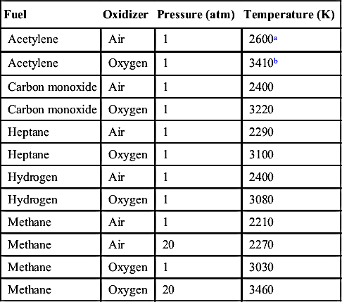
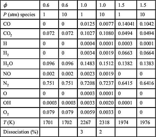
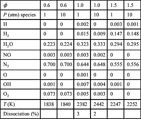
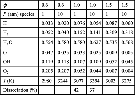
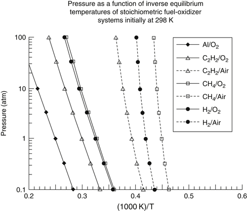
As the pressure is increased in a combustion system, the amount of dissociation decreases and the temperature rises, as shown in Figure 1.6. This observation follows directly from Le Chatelier's principle. The effect is greatest, of course, at the stoichiometric air–fuel mixture ratio where the amount of dissociation is greatest. In a system that has little dissociation, the pressure effect on temperature is small. As one proceeds to a very lean operation, the temperatures and degree of dissociation are very low compared to the stoichiometric values; thus the temperature rise due to an increase in pressure is also very small. Figure 1.6 reports the calculated stoichiometric flame temperatures for propane and hydrogen in air and in pure oxygen as a function of pressure. Tables 1.3–1.6 list the product compositions of these fuels (in mole fractions) for three stoichiometries and pressures of 1 and 10 atm. As will be noted in Tables 1.3 and 1.5, the dissociation is minimal, amounting to about 3% at 1 atm and 2% at 10 atm. Thus one would not expect a large rise in temperature for this 10-fold increase in pressure, as indeed Tables 1.3 and 1.5 and Figure 1.6 reveal. This small variation is due mainly to the presence of large quantities of inert nitrogen. The results for pure oxygen (Tables 1.4 and 1.5) show a substantial degree of dissociation and about a 15% rise in temperature as the pressure increases from 1 to 10 atm. The effect of nitrogen as a diluent can be noted from Table 1.2, where the maximum flame temperatures of various fuels in air and pure oxygen are compared. Comparisons for methane in particular show very interesting effects. First, at 1 atm for pure oxygen the temperature rises about 37%; at 20 atm, over 50%. The rise in temperature for the methane–air system as the pressure is increased from 1 to 20 atm is only 2.7%, whereas for the oxygen system over the same pressure range the increase is about 14.2%. Again, these variations are due to the differences in the degree of dissociation. The dissociation for the equilibrium calculations is determined from the equilibrium constants of formation; moreover, from Le Chatelier's principle, the higher the pressure the lower the amount of dissociation. Thus it is not surprising that a plot of ln Ptotal versus (1/Tf) gives mostly straight lines, as shown in Figure 1.7. Recall that the equilibrium constant is equal to exp(−ΔG°/RT).
Figure 1.5Equivalence ratio ϕ = 1.1 values of Figure 1.3 on an expanded scale.
Figure 1.6Calculated stoichiometric flame temperatures of propane and hydrogen in air and oxygen as a function of pressure.
Table 1.2
Approximate Flame Temperatures of Various Stoichiometric Mixtures, Initial Temperature 298 K
Equilibrium Product Composition of Propane–Air Combustion
ϕ
0.6
0.6
1.0
1.0
1.5
1.5
P (atm) species
1
10
1
10
1
10
CO
0
0
0.0125
0.0077
0.14041
0.1042
CO2
0.072
0.072
0.1027
0.1080
0.0494
0.0494
H
0
0
0.0004
0.0001
0.0003
0.0001
H2
0
0
0.0034
0.0019
0.0663
0.0664
H2O
0.096
0.096
0.1483
0.1512
0.1382
0.1383
NO
0.002
0.002
0.0023
0.0019
0
0
N2
0.751
0.751
0.7208
0.7237
0.6415
0.6416
O
0
0
0.0003
0.0001
0
0
OH
0.0003
0.0003
0.0033
0.0020
0.0001
0
O2
0.079
0.079
0.0059
0.0033
0
0
T (K)
1701
1702
2267
2318
1974
1976
Dissociation (%)
3
2
Table 1.4
Equilibrium Product Composition of Propane–Oxygen Combustion
ϕ
0.6
0.6
1.0
1.0
1.5
1.5
P (atm) species
1
10
1
10
1
10
CO
0.090
0.078
0.200
0.194
0.307
0.313
CO2
0.165
0.184
0.135
0.151
0.084
0.088
H
0.020
0.012
0.052
0.035
0.071
0.048
H2
0.023
0.016
0.063
0.056
0.154
0.155
H2O
0.265
0.283
0.311
0.338
0.307
0.334
O
0.054
0.041
0.047
0.037
0.014
0.008
OH
0.089
0.089
0.095
0.098
0.051
0.046
O2
0.294
0.299
0.097
0.091
0.012
0.008
T (K)
2970
3236
3094
3411
3049
3331
Dissociation (%)
27
23
55
51
Table 1.5
Equilibrium Product Composition of Hydrogen–Air Combustion
ϕ
0.6
0.6
1.0
1.0
1.5
1.5
P (atm) species
1
10
1
10
1
10
H
0
0
0.002
0
0.003
0.001
H2
0
0
0.015
0.009
0.147
0.148
H2O
0.223
0.224
0.323
0.333
0.294
0.295
NO
0.003
0.003
0.003
0.002
0
0
N2
0.700
0.700
0.644
0.648
0.555
0.556
O
0
0
0.001
0
0
0
OH
0.001
0
0.007
0.004
0.001
0
O2
0.073
0.073
0.005
0.003
0
0
T (K)
1838
1840
2382
2442
2247
2252
Dissociation (%)
3
2
Table 1.6
Equilibrium Product Composition of Hydrogen–Oxygen Combustion
ϕ
0.6
0.6
1.0
1.0
1.5
1.5
P (atm) species
1
10
1
10
1
10
H
0.033
0.020
0.076
0.054
0.087
0.060
H2
0.052
0.040
0.152
0.141
0.309
0.318
H2O
0.554
0.580
0.580
0.627
0.535
0.568
O
0.047
0.035
0.033
0.025
0.009
0.005
OH
0.119
0.118
0.107
0.109
0.052
0.045
O2
0.205
0.207
0.052
0.044
0.007
0.004
T (K)
2980
3244
3077
3394
3003
3275
Dissociation (%)
42
37
Figure 1.7The variation of the stoichiometric flame temperature of various fuels in air and oxygen as a function of pressure in the form log P versus (1/Tf), where the initial temperature is 298 K.
Many experimental systems in which nitrogen may undergo some reactions employ artificial air systems, replacing nitrogen with argon on a mole-for-mole basis. In this case the argon system creates much higher system temperatures because it absorbs much less of the heat of reaction owing to its lower specific heat as a monatomic gas. The reverse is true, of course, when the nitrogen is replaced with a triatomic molecule such as carbon dioxide. Appendix B provides the adiabatic flame temperatures for stoichiometric mixtures of hydrocarbons and air for fuel molecules as large as C16 further illustrating the discussions of this section.
Since some heat loss is present in all real environments, temperatures in combustion systems calculated using the adiabatic equilibrium approach defined in this chapter are often considered to be representative of the maximum possible temperatures in a given combustion system. However, systems that are not in chemical equilibrium are not necessarily constrained to temperatures below the adiabatic equilibrium temperature. In particular, measurements in flames in which product species such as H2 and H2O have not fully dissociated have yielded ‘superadiabatic’ temperatures several hundred degrees Celsius above the adiabatic equilibrium temperature. These temperatures persist well beyond the initial flame zone. The most common systems in which this effect has been observed are the very fuel-rich hydrocarbon flames. The effect has also been seen in ammonia flames. Chemical kinetics, discussed in Chapters 2 and 3, are responsible for the temperature overshoot, and in particular the degree of chain branching, the change in moles across the reaction, and whether the system approaches the final equilibrium state through overall dissociation or recombination. The phenomenon is predictable using detailed combustion kinetics models [11–12] and has been measured experimentally with multiple methods [13–14].
1.5. Sub and Supersonic Combustion Thermodynamics
1.5.1. Comparisons
In Chapter 4, Section 4.8, the concept of stabilizing a flame in a high-velocity stream is discussed. This discussion is related to streams that are subsonic. In essence what occurs is that the fuel is injected into a flowing stream and chemical reaction occurs in some type of flame zone. These types of chemically reacting streams are most obvious in air-breathing engines, particularly ramjets. In ramjets flying at supersonic speeds, the air intake velocity must be lowered such that the flow velocity is subsonic entering the combustion chamber where the fuel is injected and the combustion stabilized by some flame-holding technique. The inlet diffuser in this type of engine plays a very important role in the overall efficiency of the complete thrust-generating process. Shock waves occur in the inlet when the vehicle is flying at supersonic speeds. Since there is a stagnation pressure loss with this diffuser process, the inlet to a ramjet must be carefully designed. At very high supersonic speeds, the inlet stagnation pressure losses can be severe. It is the stagnation pressure at the inlet to the engine exhaust nozzle which determines an engine's performance. Thus the concept of permitting complete supersonic flow through a properly designed converging–diverging inlet to enter the combustion chamber where the fuel must be injected, ignited, and stabilized requires a condition that the reaction heat release takes place in a reasonable combustion chamber length. In this case, a converging–diverging section is still required to provide a thrust-bearing surface. Whereas it will become evident in later chapters that normally the ignition time is much shorter than the time to complete combustion in a subsonic condition, in the supersonic case the reverse could be true. Thus there are three types of stagnation pressure losses in these subsonic and supersonic (scramjet) engines. They are due to inlet conditions, the stabilization process, and the combustion (heat release) process. As will be shown subsequently, although the inlet losses are smaller for the scramjet, stagnation pressure losses are greater in the supersonic combustion chamber. Stated in a general way, for a scramjet to be viable as a competitor to a subsonic ramjet, the scramjet must fly at very high Mach numbers where the inlet conditions for the subsonic case would cause large stagnation pressure losses. Even though inlet aerodynamics are outside the scope of this text, it is appropriate to establish in this chapter related to thermodynamics why subsonic combustion produces a lower stagnation pressure loss compared to supersonic combustion. This approach is possible since only the extent of heat release (enthalpy) and not the analysis of the reacting system is required. In a supersonic combustion chamber, developing a stabilization technique that minimizes losses while still permitting rapid ignition remains a challenging endeavor.
1.5.2. Stagnation Pressure Considerations
To understand the difference in stagnation pressure losses between subsonic and supersonic combustion one must consider sonic conditions in isoergic and isentropic flows; that is, one must deal with, as is done in fluid mechanics, the Fanno and Rayleigh lines. Following an early NACA report for these conditions, since the mass flow rate (ρuA) must remain constant, then for a constant area duct the momentum equation takes the form
(dP/ρ)=−u2(du/u)=−a2M2(du/u)
where a² is the speed of sound squared defined as
a2=(∂P∂ρ)s
M is the Mach number. For the condition of flow within a variable area duct, in essence the equation simply becomes
(1−M2)(dP/ρ)=a2M2(dA/A)=u2(dA/A)
(1.60)
where A is the cross-sectional area of the flow chamber. For dA = 0 which is the condition at the throat of a nozzle it follows from Eqn (1.60) either dP = 0 or M = 1. Consequently, a minimum or maximum is reached, except when the sonic value is established in the throat of the nozzle. In this case the pressure gradient can be different. It follows then
(dP/dA)=[a2M2/(1−M2)](ρ/A)
(1.61)
For M > 1, (dP/dA) < 0 and for M < 1, (dP/dA) > 0; that is, the pressure falls as one expands the area in supersonic flow and rises in subsonic flow.
For adiabatic flow in a constant area duct, that is ρu = constant, one has for the Fanno line
h+(u2/2)=h°
where the lower case h is the enthalpy per unit mass, and the superscript o denotes the stagnation or total enthalpy. Considering P as a function of ρ and s (entropy), using Maxwell's thermodynamic relations, the earlier definition of the sound speed and, for the approach here, the entropy as noted by
Tds=dh−(dP/ρ)
the expression of the Fanno line takes the form
(dh/ds)f=[M2/(M2−1)]T[1+(∂lnT/∂lnρ)s]
(1.62)
Since T varies in the same direction as ρ in an isotropic change, the term in brackets is positive.
Thus for the flow conditions
(dh/ds)f>0forM>1
(dh/ds)f<0forM<1
(dh/ds)f=∞forM=1(soniccondition)
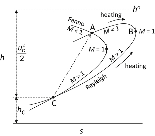
where the subscript f denotes the Fanno condition. This derivation permits the Fanno line to be detailed in Figure 1.8 which also contains the Rayleigh line to be discussed.
The Rayleigh line is defined by the condition which results from heat exchange in a flow system and requires that the flow force remain constant, in essence for a constant area duct the condition can be written as
dP+(ρu)du=0
For a constant area duct note that
Figure 1.8An overlay of Fanno–Rayleigh conditions.
(dρ/ρ)+(du/u)=0
Again following the use of Eqns (1.61) and (1.62), the development that ensues leads to
(dh/ds)r=[T/(M2−1)]{[1+(∂lnT/∂lnρ)s]M2−1}
(1.63)
where the subscript r denotes the Rayleigh condition. Examining Eqn (1.63), one will first note that at M = 1, (dh/ds)r = ∞, but also at some value of M < 1 the term in the braces could equal 0 and thus (dh/ds) = 0. Thus between this value and M = 1, (dh/ds)r < 0. At a value of M still less than the value for (dh/ds)r = 0, the term in braces becomes negative and with the negative term multiple of the braces, (dh/ds)r becomes > 0. These conditions determine the shape of the Rayleigh line which is shown in Figure 1.8 with the Fanno line.
The conservation equations for a normal shock are represented by the Rayleigh and Fanno conditions. The downstream state (or final point) of a normal shock is fixed by the intersection of both lines (point A of Figure 1.8) passing through the upstream state (or initial point C). Because the entropy at point A is greater than at point C, flow across the shock passes from C to A and thus the velocity changes from supersonic before the shock to subsonic after the shock. Since heat addition in a constant area duct cannot raise the velocity of the reacting fluid past the sonic speed, Figure 1.8 represents the entropy change for both subsonic and supersonic flow for the same initial stagnation enthalpy. Equation (1.28) written in mass units can be represented as
Δs=−R′Δ(lnP)
It is apparent the smaller change in entropy of subsonic combustion (A to B in Figure 1.8) compared to supersonic combustion (C to B) establishes that there is a lower stagnation pressure loss in the subsonic case compared to the supersonic case. To repeat, for a scramjet to be viable, the inlet losses at the very high Mach number for subsonic combustion must be large enough to override its advantages gained in its energy release.
Problems
(Those with an asterisk require a numerical solution and use of an appropriate software program—See Appendix I.)
1. Suppose that methane and air in stoichiometric proportions are brought into a calorimeter at 500 K. The product composition is brought to the ambient temperature (298 K) by the cooling water. The pressure in the calorimeter is assumed to remain at 1 atm, but the water formed has condensed. Calculate the heat of reaction.
2. Calculate the flame temperature of normal octane (liquid) burning in air at an equivalence ratio of 0.5. For this problem assume there is no dissociation of the stable products formed. All reactants are at 298 K and the system operates at a pressure of 1 atm. Compare the results with those given by the graphs in the text. Explain any differences.
3. Carbon monoxide is oxidized to carbon dioxide in an excess of air (1 atm) in an afterburner so that the final temperature is 1300 K. Under the assumption of no dissociation, determine the air–fuel ratio required. Report the results on both a molar and mass basis. For the purposes of this problem assume that air has the composition of 1 mol of oxygen to 4 mol of nitrogen. The carbon monoxide and air enter the system at 298 K.
4. The exhaust of a carbureted automobile engine, which is operated slightly fuel-rich, has an efflux of unburned hydrocarbons entering the exhaust manifold. Assume that all the hydrocarbons are equivalent to ethylene (C2H4) and all the remaining gases are equivalent to inert nitrogen (N2). On a molar basis there are 40 mol of nitrogen for every mole of ethylene. The hydrocarbons are to be burned over an oxidative catalyst and converted to carbon dioxide and water vapor only. In order to accomplish this objective, ambient (298 K) air must be injected into the manifold before the catalyst. If the catalyst is to be maintained at 1000 K, how many moles of air per mole of ethylene must be added if the temperature of the manifold gases before air injection is 400 K, and the composition of air is 1 mol of oxygen to 4 mol of nitrogen?
5. A combustion test was performed at 20 atm in a hydrogen–oxygen system. Analysis of the combustion products, which were considered to be in equilibrium, revealed the following:
Compound
Mole Fraction
H2O
0.493
H2
0.498
O2
0
O
0
H
0.020
OH
0.005
What was the combustion temperature in the test?
6. Whenever carbon monoxide is present in a reacting system, it is possible for it to disproportionate into carbon dioxide according to the equilibrium
2CO⇄Cs+CO2
Assume that such an equilibrium can exist in some crevice in an automotive cylinder or manifold. Determine whether raising the temperature decreases or increases the amount of carbon present. Determine the Kp for this equilibrium system and the effect of raising the pressure on the amount of carbon formed.
7. Determine the equilibrium constant Kp at 1000 K for the following reaction:
2CH4⇄2H2+C2H4
8. The atmosphere of Venus is said to contain 5% carbon dioxide and 95% nitrogen by volume. It is possible to simulate this atmosphere for Venus reentry studies by burning gaseous cyanogen (C2N2) and oxygen and diluting with nitrogen in the stagnation chamber of a continuously operating wind tunnel. If the stagnation pressure is 20 atm, what is the maximum stagnation temperature that could be reached while maintaining Venus atmosphere conditions? If the stagnation pressure was 1 atm, what would the maximum temperature be? Assume all gases enter the chamber at 298 K. Take the heat of formation of cyanogen as (ΔH°f)298=374kJ/mol.
9. A mixture of 1 mol of N2 and 0.5 mol O2 is heated to 4000 K at 0.5 atm, affording an equilibrium mixture of N2, O2, and NO only. If the O2 and N2 were initially at 298 K and the process is one of steady heating, how much heat is required to bring the final mixture to 4000 K on the basis of one initial mole of N2?
10. Calculate the adiabatic decomposition temperature of benzene under the constant pressure condition of 20 atm. Assume that benzene enters the decomposition chamber in the liquid state at 298 K and decomposes into the following products: carbon (graphite), hydrogen, and methane.
11. Calculate the flame temperature and product composition of liquid ethylene oxide decomposing at 20 atm by the irreversible reaction
C2H4O(liq)→aCO+bCH4+cH2+dC2H4
The four products are as specified. The equilibrium known to exist is
2CH4⇄2H2+C2H4
The heat of formation of liquid ethylene oxide is
ΔH°f,298=−76.7kJ/mol
It enters the decomposition chamber at 298 K.
12. Liquid hydrazine (N2H4) decomposes exothermically in a monopropellant rocket operating at 100 atm chamber pressure. The products formed in the chamber are N2, H2, and ammonia (NH3) according to the irreversible reaction
N2H4(liq)→aN2+bH2+cNH3
Determine the adiabatic decomposition temperature and the product composition a, b, and c. Take the standard heat of formation of liquid hydrazine as 50.07 kJ/mol. The hydrazine enters the system at 298 K.
13. Gaseous hydrogen and oxygen are burned at 1 atm under the rich conditions designated by the following combustion reaction:
O2+5H2→aH2O+bH2+cH
The gases enter at 298 K. Calculate the adiabatic flame temperature and the product composition a, b, and c.
14. The liquid propellant rocket combination nitrogen tetroxide (N2O4) and UDMH (unsymmetrical dimethyl hydrazine) has optimum performance at an oxidizer-to-fuel weight ratio of two at a chamber pressure of 67 atm. Assume that the products of combustion of this mixture are N2, CO2, H2O, CO, H2, O, H, OH, and NO. Write down the equations necessary to calculate the adiabatic combustion temperature and the actual product composition under these conditions. These equations should contain all the numerical data in the description of the problem and in the tables in the appendices. The heats of formation of the reactants are
The propellants enter the combustion chamber at 298 K.
15. Consider a fuel burning in inert airs and oxygen where the combustion requirement is only 0.21 mol of oxygen. Order the following mixtures as to their adiabatic flame temperatures with the given fuel:
a. pure O2
b. 0.21 O2 + 0.79 N2 (air)
c. 0.21 O2 + 0.79 Ar
d. 0.21 O2 + 0.79 CO2
16. Propellant chemists have proposed a new high energy liquid oxidizer, penta-oxygen O5, which is also a monopropellant. Calculate the monopropellant decomposition temperature at a chamber pressure of 10 atm if it assumed the only products are O atoms and O2 molecules. The heat of formation of the new oxidizer is estimated to be very high, +1025 kJ/mol. Obviously, the amounts of O2 and O must be calculated for 1 mol of O5 decomposing. The O5 enters the system at 298 K. Hint: The answer will lie somewhere between 4000 and 5000 K.
17. Exhaust gas, which is assumed to consist of CO2, CO, H2O, O2, and N2, exit a combustor at 2500 K and 2 bar. Measurements of CO2 and O2 indicate mole fractions of 0.09 and 0.028, respectively. Assuming equilibrium conditions between CO and CO2, determine the CO mole fraction and estimate the equivalence ratio of the propane air mixture entering the combustor.
18. ∗Determine the amount of CO2 and H2O dissociation in a mixture initially consisting of 1 mol of CO2, 2 mol of H2O, and 7.5 mol of N2 at temperatures of 1000, 2000, and 3000 K at atmospheric pressure and 50 atm. Use a numerical program such as the NASA Glenn Chemical Equilibrium Analysis (CEA) program or one included with CHEMKIN (Equil for CHEMKIN II and III, Equilibrium-Gas for CHEMKIN IV). Appendix I provides information on several of these programs.
19. ∗Calculate the constant pressure adiabatic flame temperature and equilibrium composition of stoichiometric mixtures of methane (CH4) and gaseous methanol (CH3OH) with air initially at 300 K and 1 atm. Compare the mixture compositions and flame temperatures and discuss the trends.
20. ∗Calculate the adiabatic flame temperature of a stoichiometric methane–air mixture for a constant pressure process. Compare and discuss this temperature to those obtained when the N2 in the air has been replaced with He, Ar, and CO2. Assume the mixture is initially at 300 K and 1 atm.
21. ∗Consider a carbon monoxide and air mixture undergoing constant pressure, adiabatic combustion. Determine the adiabatic flame temperature and equilibrium mixture composition for mixtures with equivalence ratios varying from 0.5 to 3 in increments of 0.5. Plot the temperature and concentrations of CO, CO2, O2, O, and N2 as a function of equivalence ratio. Repeat the calculations with a 33% CO/67% H2 (by volume) fuel mixture. Plot the temperature and concentrations of CO, CO2, O2, O, N2, H2, H2O, OH, and H. Compare the two systems and discuss the trends of temperature and species concentration.
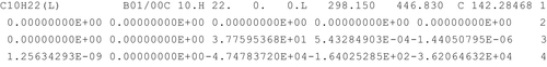
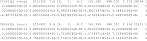
22. ∗A Diesel engine with a compression ratio of 20:1 operates on liquid decane (C10H22) with an overall air/fuel (massair/massfuel) mixture ratio of 18:1. Assuming isentropic compression of air initially at 298 K and 1 atm followed by fuel injection and combustion at constant pressure, determine the equilibrium flame temperature and mixture composition. Include NO and NO2 in the equilibrium calculations. In the NASA CEA program, equilibrium calculations for fuels, which will not exist at equilibrium conditions, can be performed with knowledge of only the chemical formula and the heat of formation. The heat of formation of liquid decane is −301.04 kJ/mol. In other programs, such as CHEMKIN, thermodynamic data are required for the heat of formation, entropy, and specific heat as a function of temperature. Such data are often represented as polynomials to describe the temperature dependence. In the CHEMKIN thermodynamic database (adopted from the NASA Chemical Equilibrium code, Gordon, S., and McBride, B. J., NASA Report SP-273, 1971), the specific heat, enthalpy, and entropy are represented by the following expressions:
Cp/Ru=a1+a2T+a3T2+a4T3+a5T4
H°/RuT=a1+a2T/2+a3T2/3+a4T3/4+a5T4/5+a6/T
S°/Ru=a1lnT+a2T+a3T2/2+a4T3/4+a5T4/5+a7
The coefficients a1 through a7 are generally provided for both high and low temperature ranges. Thermodynamic data in CHEMKIN format for liquid decane is given below.
In the data above, the first line provides the chemical name, a comment, the elemental composition, the phase, and the temperature range over which the data are reported (low temperature limit, high temperature limit, and the middle point temperature that separates the range). In lines 2 through 4, the high-temperature coefficients a1,…, a7 are presented first followed by the low-temperature coefficients. In this particular example, only the coefficients for the low-temperature range (from 298.15 to 446.83 K) are provided. For more information, refer to Kee et al. (Kee, R.J., Rupley, F.M., and Miller, J.A., “The Chemkin Thermodynamic Data Base,” Sandia Report, SAND87-8215B, reprinted March 1991).
23. ∗A spark ignition engine with a 8:1 compression ratio is tested with a reference fuel mixture consisting of 87% iso-octane (i-C8H18) and 13% normal-heptane (n-C7H16) by volume. Assuming combustion takes place at constant volume with air that has been compressed isentropically, calculate the equilibrium flame temperature and mixture composition for a stoichiometric mixture. Include NO and NO2 in the equilibrium calculation. The heats of formation of liquid iso-octane and n-heptane are −250.26 and −224.35 kJ/mol, respectively. If necessary, the thermodynamic data in CHEMKIN format are provided below. See question 22 for a description of these values.


 (1.5)
(1.5) (1.10)
 (1.11)
 (1.17)
 (1.18)
 (1.19)
 (1.30)
 (1.33)
 (1.37)
 (1.47)
 (1.48)


 (v)
(v) (vi)
(vi)
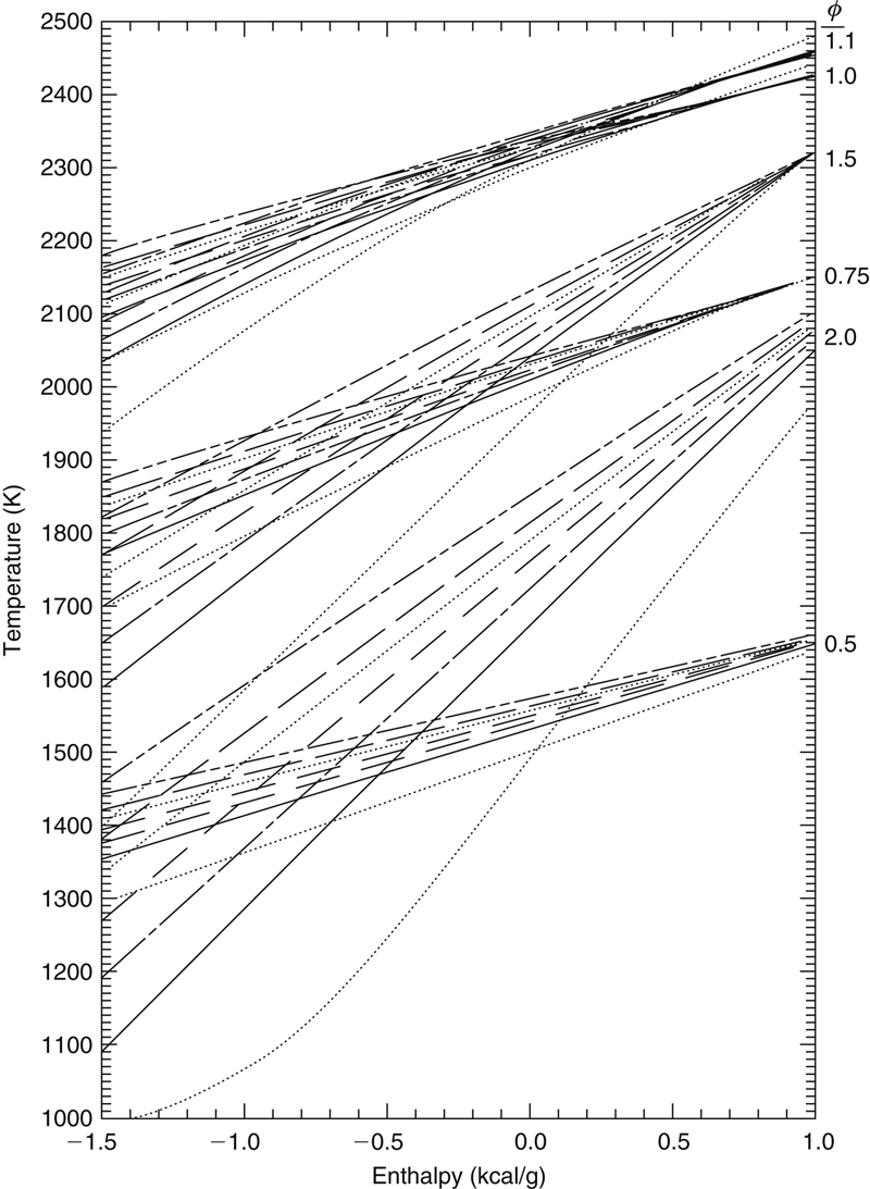
 H/C = 4;
  H/C = 3;
  H/C = 2.5;
 H/C = 2.0;
  H/C = 1.5;
  H/C = 1.0;
  H/C = 0.