Chapter 10: A Guide to Meshing in SOLIDWORKS

Meshing is the process of discretizing a structure into smaller, finite substructures. As you will have observed from past chapters, a strong interplay exists between meshing and results obtained from finite element analysis. For this reason, we will use this chapter to complete our exploration of finite element simulation for static analysis by taking a careful look at ways to customize the meshing of a structure to achieve reliable results. You will encounter mesh control (again) and learn how to employ convergence analysis to evaluate the accuracy of simulation results. In pursuit of these ideas, the remainder of the chapter entails discussion centered around the following topics:

• Discretization with beam and truss elements
• Mesh control with plane elements
• Mesh control with three-dimensional elements
• Discretization with h- and p-elements

Technical requirements

You will need to have access to the SOLIDWORKS software with a SOLIDWORKS Simulation license.

You can find the folder containing the models required for this chapter here:

https://github.com/PacktPublishing/Practical-Finite-Element-Simulations-with-SOLIDWORKS-2022/tree/main/Chapter10

Discretization with beam and truss elements

We covered the discretization of structures with a collection of truss elements in Chapter 2, Analyses of Bars and Trusses, and with a collection of beam elements in Chapter 3, Analyses of Beams and Frames, and Chapter 4, Analyses of Torsionally Loaded Components. Let's briefly highlight two of the ideas covered in those past chapters:

• We discussed the characteristics of these elements in terms of degrees of freedom – specifically, that SOLIDWORKS truss element has 3 degrees of freedom per node, while the beam element has 6 degrees of freedom per node.
• We outlined a few tricks to be employed when using those elements. Specifically, for beam elements, we discussed the idea of taking advantage of critical positions under the Modeling strategy subsection in Chapter 3, Analyses of Beams and Frames.

In addition to the preceding points, there is one important distinction between these two elements that you should know. SOLIDWORKS Simulation will use multiple beam elements to discretize a single beam-like structure. However, it uses a single truss element to discretize a truss-like structure. The implication of this is that you can specify the number of beam elements to be used in a simulation through mesh control, but you cannot use mesh control for truss elements. Recall that we introduced mesh control for beams in Chapter 7, Analyses of Components with Mixed Elements, in the Part C – Meshing and running section.

To get to the heart of the preceding point, consider the problem of analyzing the suspender system displayed in Figure 10.1, which is inspired by Exercise 4.55 in the book by Hibbeler [1]. The system comprises three links and a beam that is used to support two loads, as shown in the following figure. It is necessary to determine the normal stress of the beam:

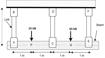
Figure 10.1 – A three-bar suspender system

In solving the problem, the links AB, DC and FE are discretized with truss elements. Next, by employing the idea of critical positions, which we covered in Chapter 3, Analyses of Beams and Frames, we would have four beam segments (AP, PC, CQ and QE) during the modeling phase. Finally, each of the beam segments will be divided into smaller beam elements as part of the discretization process.

Let's now look at a complete solution to the preceding problem, which is included in the Chapter 10 folder that you can download from this book's GitHub repository. After downloading the folder, follow these steps to examine the simulation studies:

1. Open the SOLIDWORKS part file named ThreeBars_Beam.
2. Activate SOLIDWORKS Simulation. Once the simulation add-in is activated, you will see the two studies, as shown in Figure 10.2:
   

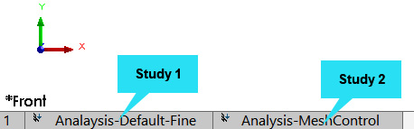
   Figure 10.2 – Static studies contained within the part file

3. Review the simulation study tree items shown in Figure 10.3. You will notice that they comprise a combination of truss and beams used for the discretization:
   

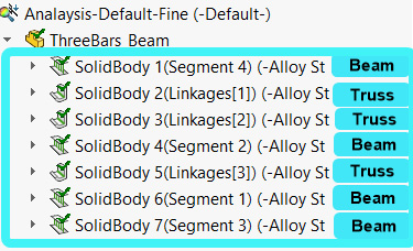
   Figure 10.3 – Discretizing with beam and truss elements

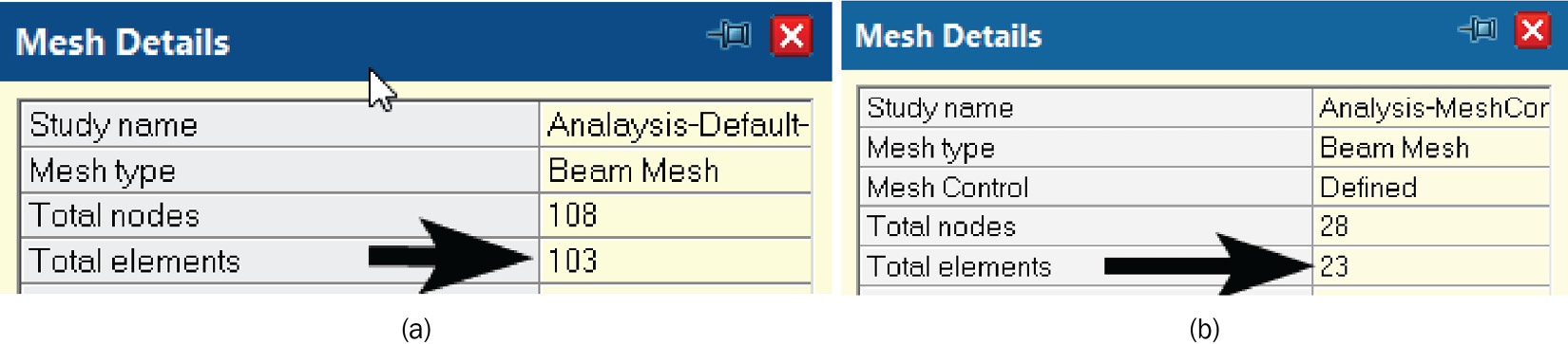
4. Review the mesh details, as shown in Figure 10.4:
   

   Figure 10.4 – (a) Study 1 mesh and (b) study 2 mesh details

5. Examine the results of bending stress from both studies, as shown in Figure 10.5:

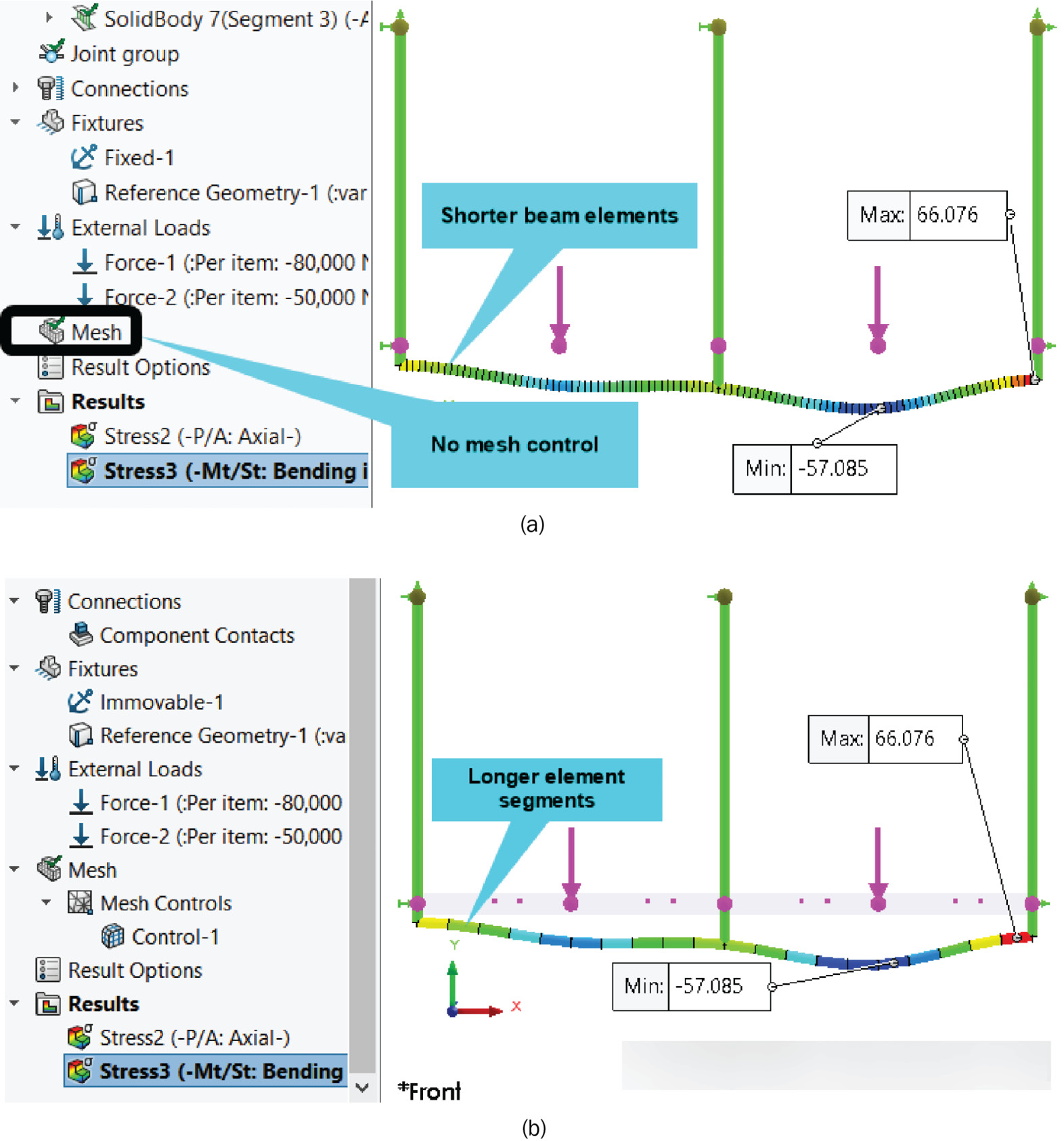
Figure 10.5 – (a) Bending stress from study 1 and (b) bending stress from study 2

What can we learn from the presented results? First, as you can see from Figure 10.4, study 1 has a total of 103 elements because we used a fine mesh, resulting in 100 shorter beam elements, plus 3 truss elements. In contrast, we utilized a moderate mesh for study 2, which yields 23 elements (20 beam elements, plus 3 truss elements). You will get 20 if you count the beam segments in Figure 10.5b.

Next, as you can see by comparing the results of the two studies depicted in Figure 10.5, the values of the maximum and minimum bending stresses from both studies are virtually the same, even though we used a reduced number of elements for study 2. Generally, it is often tempting to use a fine mesh, as done in study 1, but for large-scale structures, doing so can quickly overwhelm your system's memory. Therefore, by exploiting mesh control to customize the number of beam elements for your study, you will be able to shorten the simulation runtime in situations where you have hundreds or thousands of beam structures forming a component, as is often the case in the automotive and aerospace industries. Now, you may be wondering how then do we reconcile the number of elements to use in mesh control with the accuracy of the simulation results? The answer is premised on what is called mesh convergence, which is featured in the next section.

Mesh control with plane elements

Plane elements were introduced and discussed in Chapter 5, Analyses of Axisymmetric Bodies, where it was emphasized that they represent a two-dimensional approximation of three-dimensional continuum structures. As you will recall from that chapter, we showcased the application of the element under the Plane analysis of axisymmetric bodies subsection. Here, we will highlight the benefit of using mesh control with plane elements for an analysis that centers around plane stress. As you will know, a plane stress problem involves "a state of stress in which the normal and shear stresses directed perpendicular to the plane are assumed to be zero" [2].

Figure 10.6 is indicative of a problem that can be solved with a collection of plane elements. We shall use the determination of the maximum normal stress that develops in the component upon loading to demonstrate the importance of mesh control and convergence study:

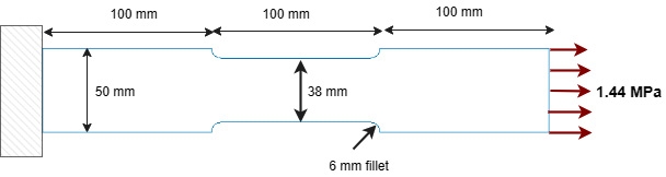
Figure 10.6 – A filleted specimen under a plane stress loading condition

To support our exploration of the concept of mesh control and convergence study, a complete solution is included in the file named PlaneStress_Bar within the Chapter 10 folder.

As we did earlier, follow these steps to examine the simulation studies:

1. Open the SOLIDWORKS part file (PlaneStress_Bar).
2. Activate SOLIDWORKS Simulation (if you are starting SOLIDWORKS afresh).

   Examine the studies, as shown in Figure 10.7. As you can see, there are seven studies within the file:

   

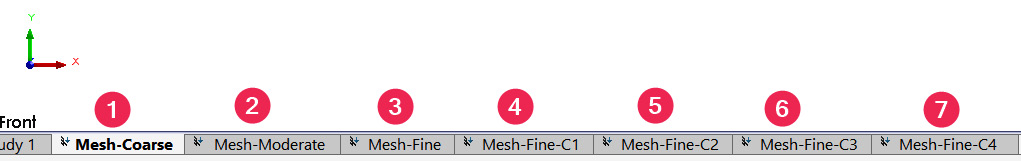
   Figure 10.7 – Seven simulation studies for the plane stress problem

3. Review the Simulation study tree items for all studies.
4. Next, review the mesh setting for each study (simply right-click the Mesh property in the Simulation study tree and choose Create Mesh).

   As you switch from one tab to another to examine the studies, you will notice that the only difference between the seven studies is the mesh quality. All other settings involving material, fixtures, and external loads are the same as presented in Figure 10.8:

   

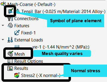
   Figure 10.8 – Simulation study tree items with plane elements

5. After examining the mesh setting, you should click Cancel to close the Mesh property manager.

   As you review the mesh setting, you will observe that we first start with a coarse mesh for the first study (Figure 10.9a), then a moderate mesh in the second study (Figure 10.9b), and then a fine mesh in the third study (Figure 10.9c). Take note of the position of the mesh slider and the element size (approximately 9.4 mm, 4.8 mm, and 2.4 mm respectively):

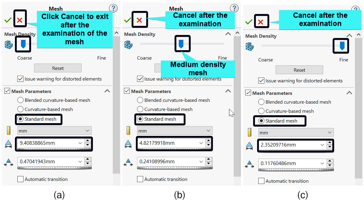
Figure 10.9 – Global mesh quality adjustment for the first three studies

For brevity's sake, the mesh details of the remaining four studies are not shown. However, they are based on the combination of the fine mesh in Figure 10.9c and mesh control features. To see the reason for the mesh control, let's review the results that correspond to the preceding three studies, as shown in Figure 10.10, depicting the distribution and maximum value of the axial normal stress:

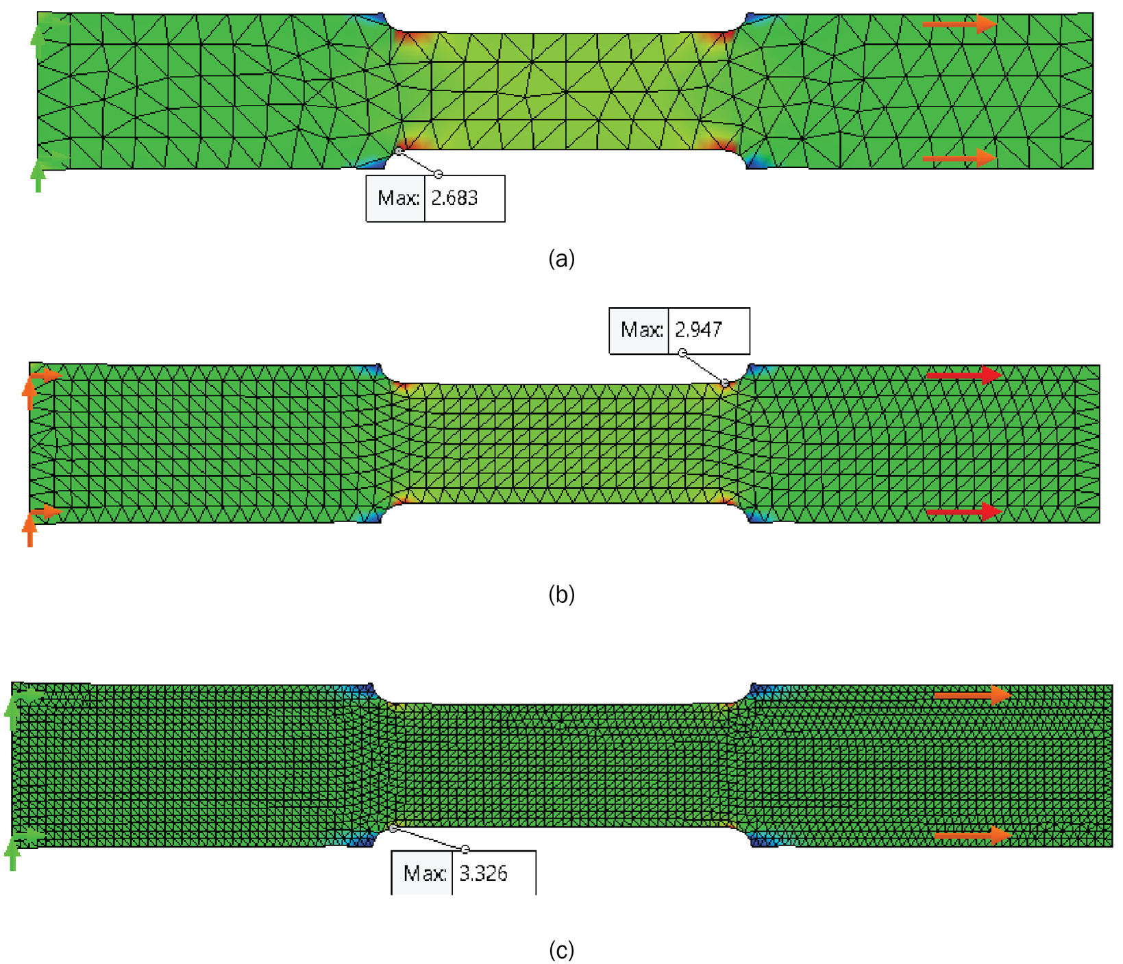
Figure 10.10 – Maximum principal stress (MPa) – (a) coarse mesh, (b) moderate mesh, and (c) fine mesh

An important insight from Figure 10.10 is that, in each stress plot, some areas exhibit a uniform and smooth color transition (mostly away from the fillets). This indicates that the mesh size is adequate to get accurate results in those regions. However, as you can see, there is a mixture of color in the regions close to the four fillets. This means the stress value has not converged in those regions. Related to this, the plots show that the value of the maximum normal stress changes as we vary the mesh size from a coarse mesh (2.683 MPa) to a fine mesh (3.326 MPa). By using local mesh control for the filleted regions, we may be able to have a better estimate of the maximum stress around the fillets. This is what we have done in the remaining four studies shown in Figure 10.7! A representative demonstration of the mesh control carried out in the last study (labeled 7 in Figure 10.7) is portrayed in Figure 10.11:

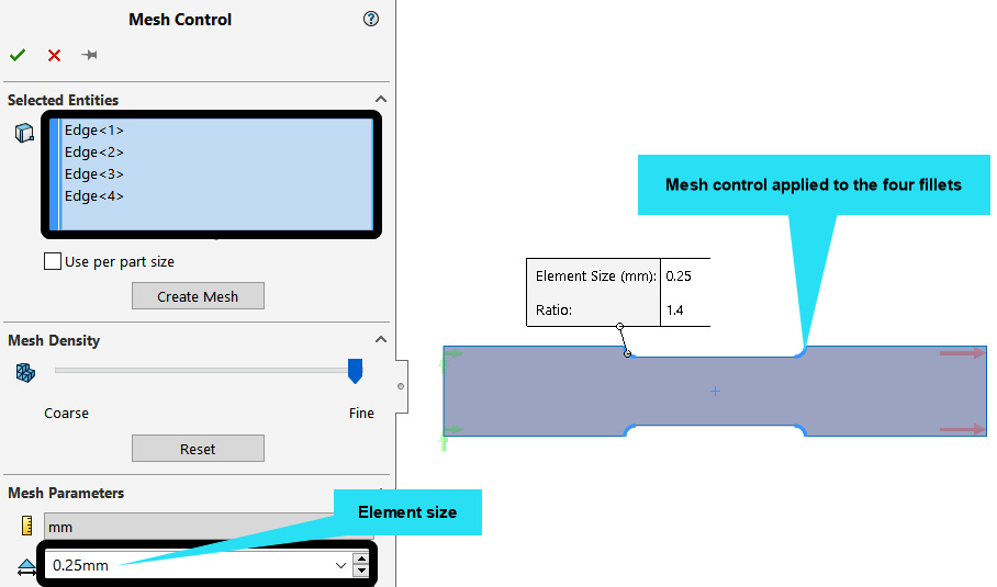
Figure 10.11 – Mesh control used for the fillets in the study named Mesh-Fine-C4

As you can see, we have specified an element size of 0.25 mm for the fillet for the aforementioned study. For the other three studies, you can check to confirm that the element size for the fillet is specified as 2 mm, 1 mm, and 0.5 mm respectively. By running the analysis for each of these mesh refinements, we can compile and tabulate the results, as shown in Table 10.12:

Table 10.12 – The variation of element size and normal stress for the seven studies

If we plot the number of elements against the maximum normal stress shown in Figure 10.12, then we can observe the trend of the curve flattening as the element number reaches close to 6,000:

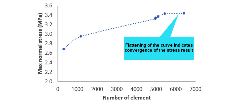
Figure 10.12 – A visualization of the convergence of results

The flattening of the curve suggests that the result is converging toward a finite value. Consequently, what we've done here is called a convergence study. It simply involves the setting up of simulation studies to observe how a particular simulation result converges toward a finite value. For static studies, a result of interest could be the maximum displacement, a specific reaction force stress value (such as principal stresses or the von-Mises stress). The plot can also be against the element size, the number of degrees of freedom, and so on. Furthermore, the mesh control can be as follows:

• Global – where the mesh is gradually refined in all areas of the structure
• Local – where the mesh refinement is focused on certain intricate features, such as holes, grooves, and fillets
• Hybrid – where the refinement takes place globally and locally

It will become obvious that the last approach is preferable in certain cases, such as in the next section, where we will orient our discussion of mesh control around solid elements.

Mesh control with three-dimensional elements

The only three-dimensional element within SOLIDWORKS Simulation is the solid element. We worked with this element in Chapter 6, Analyses of Components with Solid Elements, and Chapter 7, Analyses of Components with Mixed Elements.

As with the plane element demonstrated in the previous section, the idea of mesh control and refinement can also be applied when discretizing with solid elements. However, it is important to note that for large-scale structures, solid elements can quickly rack up degrees of freedom that will overwhelm your machine's memory. For this reason, you may find that the best compromise to arrive at a reliable result within a manageable computational time is to adopt the hybrid mesh refinement, where you combine a moderate global mesh with a locally refined mesh detail in the intricate regions. Figure 10.13 shows the difference between the number of elements and nodes for a moderate mesh (Figure 10.13a), a moderate mesh with a local mesh refinement (Figure 10.13b), a fine mesh (Figure 10.13c), and a fine mesh with local mesh refinement (Figure 10.13d):

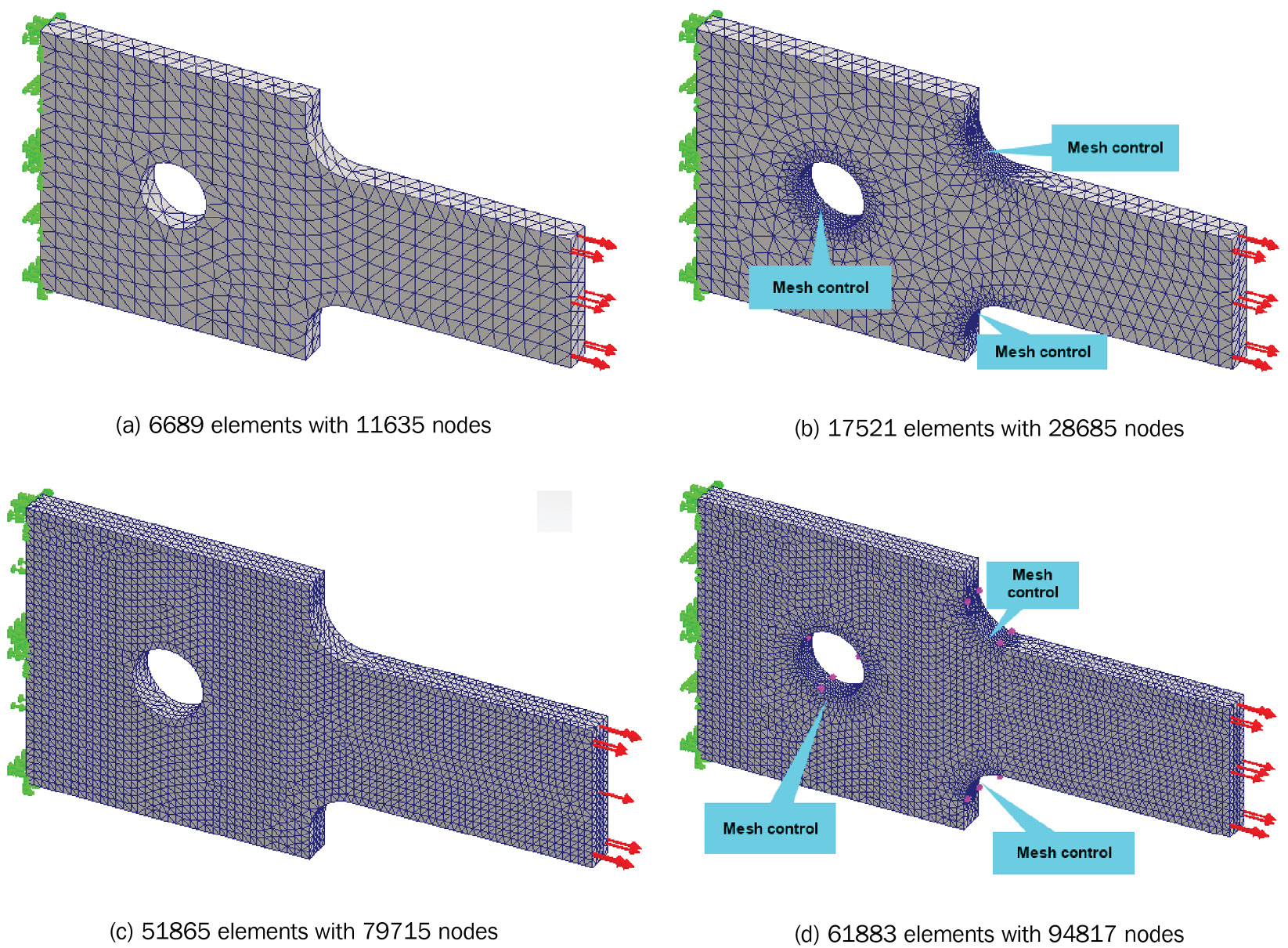
Figure 10.13 – An illustration of mesh refinements with solid elements

Let's see why a moderate global mesh with a locally refined mesh is a good compromise. You may recollect that a linear solid element has four nodes, as we mentioned in the Characteristics of solid elements subsection in Chapter 7, Analyses of Components with Mixed Elements. Each node has three Degrees of Freedom (DoF). Thus, the total degrees of freedom to be solved by adopting the linear solid elements mesh type in Figure 10.13b is 28,685 x 4, which equals 114632. Now, since finite element solutions involve matrix solutions, this means that behind the hood, the computer is solving a matrix sized 114,632 by 114,632. Now, compare this to the mesh detail in Figure 10.13d in which the total number of nodes is 94,817, resulting in a total of 379,268 DoF. For this mesh, the computer has to solve a matrix sized 379,268 by 379,268, which is more than three times the size of the matrix to be solved in Figure 10.13b. It is this increase in matrix size that contributes to a longer computational time and aggressive memory usage. Consequently, circumventing this means going with the approach of hybrid mesh control.

So, to wrap up the discussion, by adopting a moderate mesh size combined with a local mesh control, followed by a convergence study (as done in the previous section), you may be able to put some level of confidence in the accuracy of your results. There is one last remark – for very sharp corners or extremely small fillets, theoretically, you may expect an infinite value of stress (which is called stress singularity). However, it bears mentioning that there is no way to get an infinite value of stress from a finite element simulation. This is because you cannot have a mesh of size of zero! For instance, if you tried to key in zero for the mesh size parameter during meshing/mesh control, you will get an error message, as shown in Figure 10.14:

Figure 10.14 – An error from trying to enter a mesh of size zero during mesh control

This ends our discussion of meshing, mesh control, and mesh convergence study. In the last few pages, we have discussed the significance of these three concepts for one-dimensional elements (truss and beams), two-dimensional elements (plane elements), and three-dimensional elements (solid elements). Before we conclude the chapter, it may be of interest to know that apart from manually customizing the meshing detail to get accurate results, we can also employ a feature called adaptive solution methods in SOLIDWORKS Simulation. We've not covered this feature directly in the past; we shall briefly outline its essence in the next section to act as a source of further exploration for you.

Discretization with h- and p-type solution methods

The last concept we are going to call attention to is the adaptive solution method. For this, it is appropriate to begin with a brief highlight of the key parameters of the Finite Element Method (FEM). Technically, to obtain accurate solutions via finite element simulations, there are two methods of control that can be imposed to approximate the response (that is, displacement, stress, strain, and so on) of a structure:

• Control of the mesh size: As the name implies, this control is associated with reducing the mesh size, which often means that as we reduce the mesh size, and hence use more elements, it is expected that the solution will converge to a finite accurate solution.

• Control of the order of polynomial: At a fundamental level, the finite element method is a brilliant combination of the theories of polynomial approximation of differential equations and matrix analysis. Hence, controlling the order of the polynomial also tends to enhance the solution accuracy.

Altogether, the general idea is that in using polynomials to approximate a specific differential equation, we need to discretize the solution space (mesh), and then we can work with polynomials of different orders (low-order or higher-order). From this, it turns out that you can choose to find accurate solutions to a differential equation by any of the following means [3-5]:

• Fixing the mesh size while increasing the order of the approximation function, which is called the p-version of the FEM
• Fixing the order of the polynomial while decreasing the size of the mesh, which is known as the h-version of the FEM
• Using a concurrent variation of the mesh and the approximating polynomials, which is called the hp-version of the FEM

We've used the first two approaches indirectly in the past. For instance, at the beginning of Chapter 6, Analyses of Components with Solid Elements, we introduced the Mesh property manager, as shown in Figure 10.15:

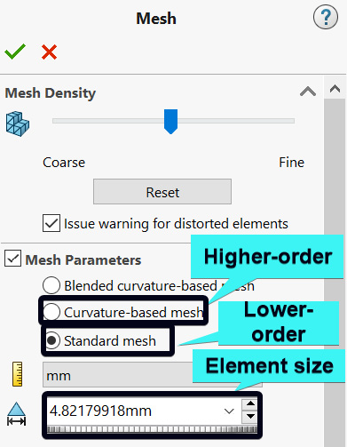
Figure 10.15 – The Mesh property manager for two- and three-dimensional elements

Essentially, switching between the Standard and Curvature-based mesh shown in Figure 10.15 is analogous to increasing the order of the polynomial interpolating function. On the other hand, by decreasing the element size, we are varying the mesh size. However, beyond the aforementioned, another way to explore the p-type and h-type approaches is via the Static Study property manager shown in Figure 10.16. To obtain the Static study property manager shown in Figure 10.16, you should right-click on a static study's name and then select Properties. This should be done before discretizing a structure that is being analyzed.

Within the Static property manager, the Adaptive tab, wedged between the Options and Flow/Thermal Effects tabs that you have explored in the past chapters, presents a choice between an h-adaptive solution and a p-adaptive solution. Selecting any of the options will expose many more options to play with. The adaptive solution methods are algorithmic and automated ways of calling on SOLIDWORKS to create mesh refinement where needed, thereby saving users the need to make decisions about where mesh refinement should be applied:

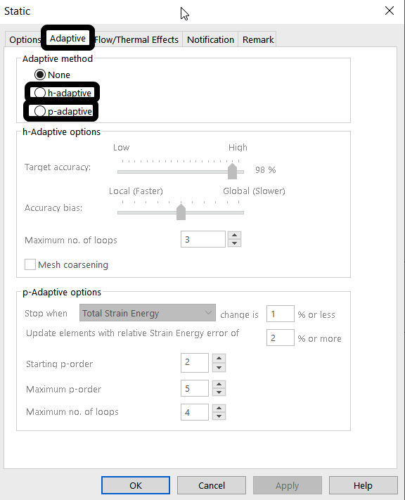
Figure 10.16 – The adaptive solution method

For further usage of the adaptive solution method, a good place to start is the online help page from SOLIDWORKS: https://help.solidworks.com/2021/English/SWConnected/cworks/IDC_HELP_PRESTATIC_P_ADAPTIVE.htm.

Overall, there is growing literature on the adaptive approach to solution refinement, and it is worth exploring it in your journey toward the mastering of advanced tricks for finite element simulation of complex structures. For elegant coverage of the mathematical concept behind the adaptive solution approach to FEM, you can check out the book by Szabó and Babuška [6].

This concludes the coverage of the topics we set out at the beginning of this chapter. In effect, the ideas we have covered in the various sections of this chapter span the strategies that underpin the accuracy of finite element simulation results. Ultimately, the discussion of this chapter should complement other important lessons that stretch across the past chapters. By building on the discourse in this chapter and the knowledge accumulated from previous chapters, it is hoped that you have solidified your understanding of some of the various powerful analyses that can be done via finite element simulations. Congratulations!

Summary

Meshing is at the heart of the finite element simulation method. To get accurate results, you must rely on a high-quality mesh and the judicious use of mesh control. For this reason, we used the various sections of this chapter to offer a short overview of procedures for the mesh refinement of different elements. Overall, we did the following:

• We revisited the discretization of truss and beam structures to demonstrate how their mesh control can be deployed to reduce computational time.
• We documented the idea of the mesh convergence study and showed how it can be employed to facilitate the accuracy of results.
• We examined the benefit of mesh control for two-dimensional and three-dimensional elements and highlighted the procedure to strike balance between the accuracy of results and gaining computational efficiency.

As this summary marks the end of the book, it is worth examining how the book has progressed. In Chapter 1, Getting Started with Finite Element Simulation, we offered an overview of FEM and introduced the uniqueness of SOLIDWORKS Simulation for the analysis of engineering components. In Chapter 2, Analyses of Bars and Trusses, we commenced the analysis journey proper with the analysis of a crane whose parts were built from weldment profiles. We extended the scope of the analysis of components built with a weldment profile in Chapter 3, Analyses of Beams and Frames. Here, we demonstrated how to employ critical points along the length of beams to create appropriate line segments, highlighted the procedure to rotate a weldment profile, and suggested ways to apply distributed and bending moment loads on beams.

In Chapter 4, Analyses of Torsionally Loaded Components, we experimented with the creation of our first custom material, worked on the analysis of components with torsional loads, and revealed how to extract an angle of twists following the application of this load. Chapter 5, Analyses of Axisymmetric Bodies, initiated our treatment of advanced elements. Primarily, we covered the attributes of shell and axisymmetric plane elements and applied these elements to two case studies in the form of pressure vessels and a flywheel. In Chapter 6, Analyses of Components with Solid Elements, as the title implies, we shifted gear to the deployment of solid elements and worked on the analysis of helical spring and spur gears (coincidentally) as case studies.

With the major family of elements covered, we brought all of them together for the analysis of a multi-story building in Chapter 7, Analyses of Components with Mixed Elements. Via the multistory building example, we showed how to use the automatic contact pairs detection tool and highlighted how to employ the SOLIDWORKS Simulation in-built soft spring to provide stability. In Chapter 8, Simulation of Components with Composite Materials, we introduced the procedure for the analysis of components with composite materials. Thermal effects, cyclical load, and design study via optimization were the focal points of Chapter 9, Simulation of Components under Thermo-Mechanical and Cyclic Loads. And, finally, we ended it all with this chapter, where we have focused on meshing.

Although we've covered a lot of ground throughout the chapters, there is still so much that remains to be learned. The truth is, the field of finite element simulation is broad, and we have only scratched the surface. Nevertheless, it is hoped that the skills you've acquired will serve as a springboard to further exploration of advanced concepts.

Further reading

• [1] Mechanics of Materials, R. C. Hibbeler, eBook, SI Edition, Pearson Education, 2017
• [2] A First Course in the Finite Element Method, D. L. Logan, Cengage Learning, 2011
• [3] The p-Version of the Finite Element Method, SIAM Journal on Numerical Analysis, Vol. 18, No. 3, I. Babuska, B. A. Szabo, and I. N. Katz, pp. 515–545, 1981
• [4] Interpolation and Quasi-Interpolation in h- and hp-Version Finite Element Spaces, Encyclopedia of Computational Mechanics Second Edition, T. Apel and J. M. Melenk, pp. 1–33, 2017
• [5] Bending of Microstructure-Dependent MicroBeams and Finite Element Implementations with R, R for Finite Element Analyses of Size-Dependent Microscale Structures, K. B. Mustapha, Springer, pp. 13–45, 2019
• [6] Finite Element Analysis: Method, Verification and Validation, B. Szabó and I. Babuška, 2021