Chapter 5: Analyses of Axisymmetric Bodies

In the previous three chapters, we dealt with the analyses of components that are analyzed using either a truss or beam element. Using these elements, we have also demonstrated the application of basic load types such as uniformly distributed load, as well as axial/transverse bending/torsional loads. Truss and beam elements provide a good entry point for exploring finite element simulations of components. However, the theoretical basis of these elements restricts their application to the analyses of components characterized by having a geometric length that is far greater than the dimensions of the cross-section. Essentially, they are good for long, straight one-dimensional structures, but they fall short for the analysis of many forms of advanced components.

In this chapter, we'll learn how to simulate components with more robust elements within the SOLIDWORKS simulation. Specifically, in this chapter, we will examine the shell element and the axisymmetric plane element. We will demonstrate how to use these elements to simulate axisymmetric bodies. In doing so, we will highlight the use of pressure load and load in the form of centrifugal speed within the SOLIDWORKS simulation environment. For this purpose, we will cover the following main topics:

• Overview of axisymmetric body problems
• Strategies for analyzing axisymmetric bodies
• Getting started with analyzing a thin-walled pressure vessel in a SOLIDWORKS simulation
• Plane analysis of axisymmetric bodies

Technical requirements

To complete this chapter, you will need to have access to the SOLIDWORKS software with a SOLIDWORKS simulation license.

You can find the sample files of the models required for this chapter here: https://github.com/PacktPublishing/Practical-Finite-Element-Simulations-with-SOLIDWORKS-2022/tree/main/Chapter05

Overview of axisymmetric body problems

A crucial aspect of engineering simulation is figuring out approximations that allow us to simplify specific problems without compromising the accuracy of our analysis. Designating certain problems as axisymmetric problems is one such approximation in the context of structural analysis.

In general, an axisymmetric body problem is characterized by two fundamental features:

• First, it involves a component that may be generated by revolving a curve or a plane section around an axis of symmetry [1] (see the Further reading section).
• Second, the component under question is assumed to have radially symmetric material properties, supports and loading configurations.

There are three important problems where the notion of axisymmetric considerations has contributed to the simplifications of analysis:

• Pressurized Vessels: This includes various kinds of vessels in the form of thin-walled/thick-walled cylindrical, conical, toroidal, and spherical pressure vessels.
• Circular Plates: This includes thin or thick circular plates that are loaded and supported axisymmetrically.
• General Three-Dimensional Solids of Revolution: This encompasses structures with radial symmetry that cannot be described as simple circular plates or pressure vessels.

Put together, these three classes of axisymmetric components play an integral part in various applications. For instance, pressure vessels are extensively used to contain and transport fluids in chemical/food/beverage processing plants and the oil and gas industries. Circular plates are deployed for use as pressure sensors, auto brake disks, nozzle covers, the end covers of pressurized vessels, the bases of storage silos, and more. Representative examples of the general 3D solid of revolution include bolt and nut assembly, aircraft fuselage, engine valve stems, turbine disks, flywheels, hyperbolic cooling towers, wheel-tire assembly, grinding wheels for completing machinery parts, and more. The following diagram shows some such examples:

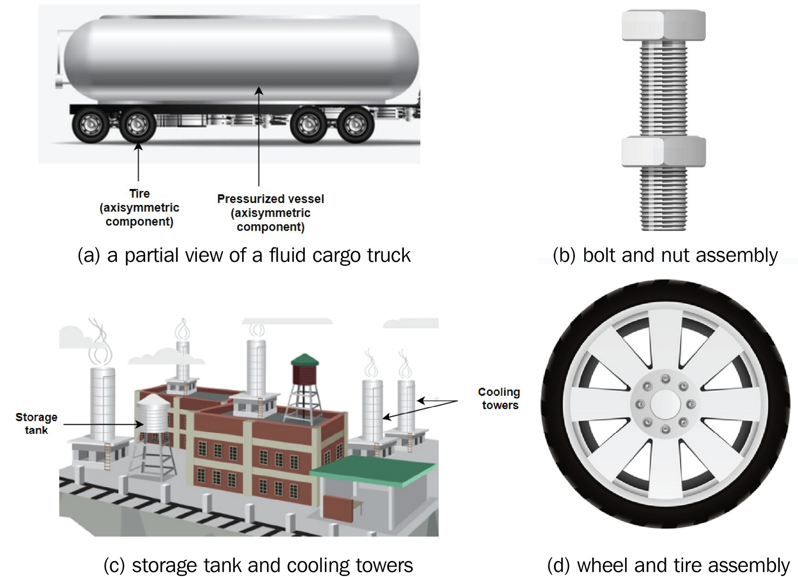
Figure 5.1 – Some examples of axisymmetric bodies

With a bit of background provided about axisymmetric components, let's discuss how we can analyze them.

Strategies for analyzing axisymmetric bodies

This section describes some modeling/analysis strategies for dealing with axisymmetric bodies. As you would have noticed from the previous chapters, before we can adopt a strategy for the modeling and simulation tasks, some structural details must be in place.

Structural details

The technical details that are needed for analyzing axisymmetric problems are no different from those of the previous chapters. These details have been reiterated here for completeness:

• The dimensions of the axisymmetric component should be provided.
• The material properties (the assumption of there being isotropic material properties has been adopted in this chapter as well) should be known.
• External loads must be applied to the axisymmetric component.
• Supports must be provided to the component to ensure its stability.

With the structural details sorted out, we need to make decisions about the modeling strategy to adopt. We will look at this next.

Modeling strategies

Analyzing axisymmetric bodies depends on a shared feature. This feature indicates that when these bodies are evaluated within the framework of a cylindrical coordinate system (characterized by r, , or z-axis), the stresses and strains that develop in these bodies during loading are independent of the circumferential coordinate . Bearing this in mind, any of the following modeling strategies can be adopted, depending on the type of axisymmetric body under consideration:

• Modeling based on the full revolved body (for example, Figures 5.2a and d): This is often very costly in terms of computational resources. For the simulation phase, the full 3D model can be analyzed by using either shell or solid elements or a combination of both. The choice of shell elements or solid elements will depend on the type of axisymmetric body under consideration.
• Modeling based on a reduced partial, symmetric partial model (for example, Figures 5.2b, c, and e): By taking advantage of the axisymmetric property, this approach lowers the duration of the simulation operation. But importantly, it minimizes the number of elements required to get relatively satisfactory results. As in the first approach, the partial 3D model can be prepared for processing with either shell or solid elements or a combination of both for complicated geometries.
• Modeling based on the use of a planar surface cross-section (for example, Figure 5.2f): This approach also reduces the computational resources needed to get satisfactory results. However, one of its significant differences compared to the preceding approaches lies in the use of a two-dimensional (2D) axisymmetric plane element:

Figure 5.2 – Modeling considerations when analyzing axisymmetric bodies: (a) Full model of a pressure vessel; (b) Sectioned model of a thin-walled pressure vessel; (c) Sectioned model of a thick-walled pressure vessel; (d) Full model of a general revolved body; (e) Quarter model of a general revolved body; (f) Plane model of a general revolved body

Meanwhile, if you wish to analyze pressure vessels (and by extension, circular plate-like axisymmetric components), it is possible to break these analysis strategies into two strands:

• An analysis that employs thin shell elements during the simulation (for thin-walled components)
• An analysis that employs thick shell elements during the simulation (for thick-walled components where the effect of shear deformation is significant and needs to be considered)

From this, the following question arises: What is the key criterion that guides the decision to use thin or thick shell elements? Principally, the choice of thin or thick shell elements has to be based on the value of the ratio of the inside diameter (Di) to the thickness (t); that is, (Di/t). In practice, you should use the following:

• Thin shell elements if Di/t > = 20
• Thick shell elements if Di/t < 20

However, for analyzing general three-dimensional revolved bodies, such as the one shown in Figure 5.2d, you either have to use solid elements or axisymmetric plane elements.

We shall deal with solid elements in Chapter 6, Analyses of Components with Solid Elements, but for now, let's examine the key features of the shell and axisymmetric plane elements.

Characteristics of shell and axisymmetric plane elements

Two case studies will be presented in this chapter. The first will involve the use of shell elements, while the second will demonstrate the use of axisymmetric plane elements. A brief discussion about the features of these elements will be provided in this section.

The shell element is technically a 2D element. Within the SOLIDWORKS simulation library, there are two formulations of this element, as shown in the following diagram:

• The first-order triangular shell element (also called a linear triangular element)
• The second-order triangular shell element with six nodes (also referred to as a parabolic triangular element):
  

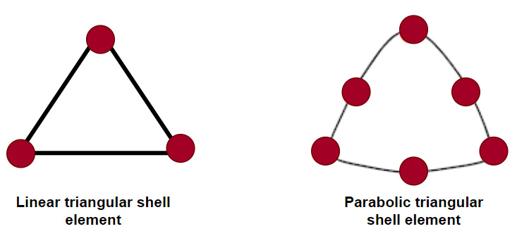
Figure 5.3 – Available shell elements in the SOLIDWORKS simulation library

Each node of the shell element shown in the preceding diagram is endowed with six degrees of freedom. These degrees of freedom are three translational displacements along the X, Y, and Z axes, and three rotational displacements about these three axes. This feature gives the shell elements the ability to resist membrane and bending loads. In practice, you will need fewer parabolic elements to accurately represent curved surfaces (compared to using linear elements).

As for the axisymmetric plane element within the SOLIDWORKS simulation library, it is similar in shape to the shell element (that is, triangular). However, it only has two degrees of freedom per node. These are principally two translational displacements in the plane of the element.

Note

There is a sound mathematical basis for these elements that can be found in many advanced textbooks on finite element analysis. There are also formulations of other non-triangular shapes in other software such as ANSYS and ABAQUS. To explore these ideas further, you may consult texts such as those by Zienkiewicz, et al. [2], Bhatti [1], and Desai [3], among others.

Now that we have highlighted the features of the elements, we will explore two case studies that will help us uncover the usage of the aforementioned elements within the SOLIDWORKS simulation environment. Along the way, some important ideas that are specific to the analysis of axisymmetric bodies will be highlighted. The next section addresses the first case study.

Getting started with analyzing thin-walled pressure vessels in a SOLIDWORKS simulation

This first case study demonstrates one of the modeling/simulation approaches for simulating thin-walled pressure vessels. As part of this demonstration, this section illustrates creating a thin surface from a thin-walled body. It also highlights how to apply pressure loads and symmetric boundary conditions. In addition, mesh refinements and methods will be provided so that you can compare the results of multiple simulation studies.

Let's get started.

Problem statement – case study 1

A thin cylindrical vessel with hemispherical heads, as depicted in the following diagram, is to be used as a gas storage tank. It is expected to withstand an internal pressure of 7 MPa. The tank is made of steel with Young's modulus of 200 GPa and a Poisson's ratio of 0.3. The internal diameter, length, and thickness of the cylinder are 75 mm, 250 mm, and 2.5 mm, respectively.

We are interested in simulating the loading of the vessel to obtain the magnitude of the principal stresses in the cylindrical section of the vessel:

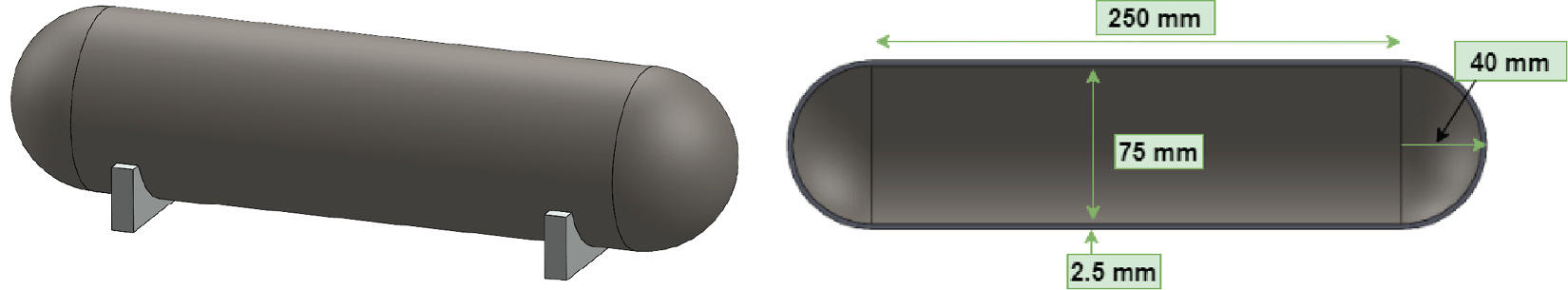
Figure 5.4 – A thin-walled pressure vessel with an internal pressure of 7 MPa

Analytical expressions exist for the principal stresses that are developed in a thin-walled cylindrical vessel with internal pressure. Nevertheless, the problem is inspired by example 9.1 in Chapter 9, Simulation of Components under Thermo-Mechanical and Cyclic Loads, in the book by Hearn [4]. In the solution, the authors obtained the values of 105 MPa and 52.4 MPa for two of the three principal stresses, because for thin-walled vessels, the third principal stress in the radial direction is often assumed to be negligibly small, and is hence neglected in theoretical evaluations. Note that we will be able to obtain the three principal stresses from our simulation. However, our focus is this: can we use the SOLIDWORKS simulation to verify the two principal stresses computed in Hearn [4]?

In an attempt to answer this question, we shall address the case study in three major sections, designated as Part A – Creating the model of the cylinder, Part B – Creating the simulation study, and Part C – Meshing. The first set of actions are related to creating the model of the cylinder, which is described in the next section.

Let's begin.

Part A – Creating a model of the cylinder

It is important to clarify a few points before we dig deep. First, when we simulate the problem at hand, we will ignore the effect of the support structures at the base of the vessel. Second, in practice, the vessel will have an opening (usually at the top). This will also be ignored. These two simplifications are necessary to get the result of the simulation to align with the theory of thin-walled pressure vessels [5] (see the Further reading section). In other words, we will be focusing on the resistance of the vessel's walls going forward. Consequently, we only need to create a model of the vessel.

Note

In practice, we could create a model that will contain the support structures and the openings. Then, for simplification during the simulation task, these features can be suppressed. A brief explanation of suppressing features during simulation can be found in Chapter 6, Analyses of Components with Solid Elements.

Furthermore, we can employ either a full model or a partial symmetric model of the vessel. Now, since we aim to demonstrate the simplification afforded by the axisymmetric condition, we shall adopt a partial symmetric model of the cylinder. Therefore, this subsection will focus on creating this partial model.

To commence, fire up SOLIDWORKS (File  New  Part). You are encouraged to save the file as Cylinder and ensure that the unit is set to the MMGS unit system.

Creating the revolving profile

The steps that follow aim to create the profile that will be revolved to form the geometric model of the pressure vessel. This profile is sketched on the Top Plane area (note that this is just a preference; you may as well use the front plane). Start by following these steps:

1. Navigate to the Sketch tab.
2. Click on the Sketch tool.
3. Choose Top Plane, as shown in the following screenshot:
   

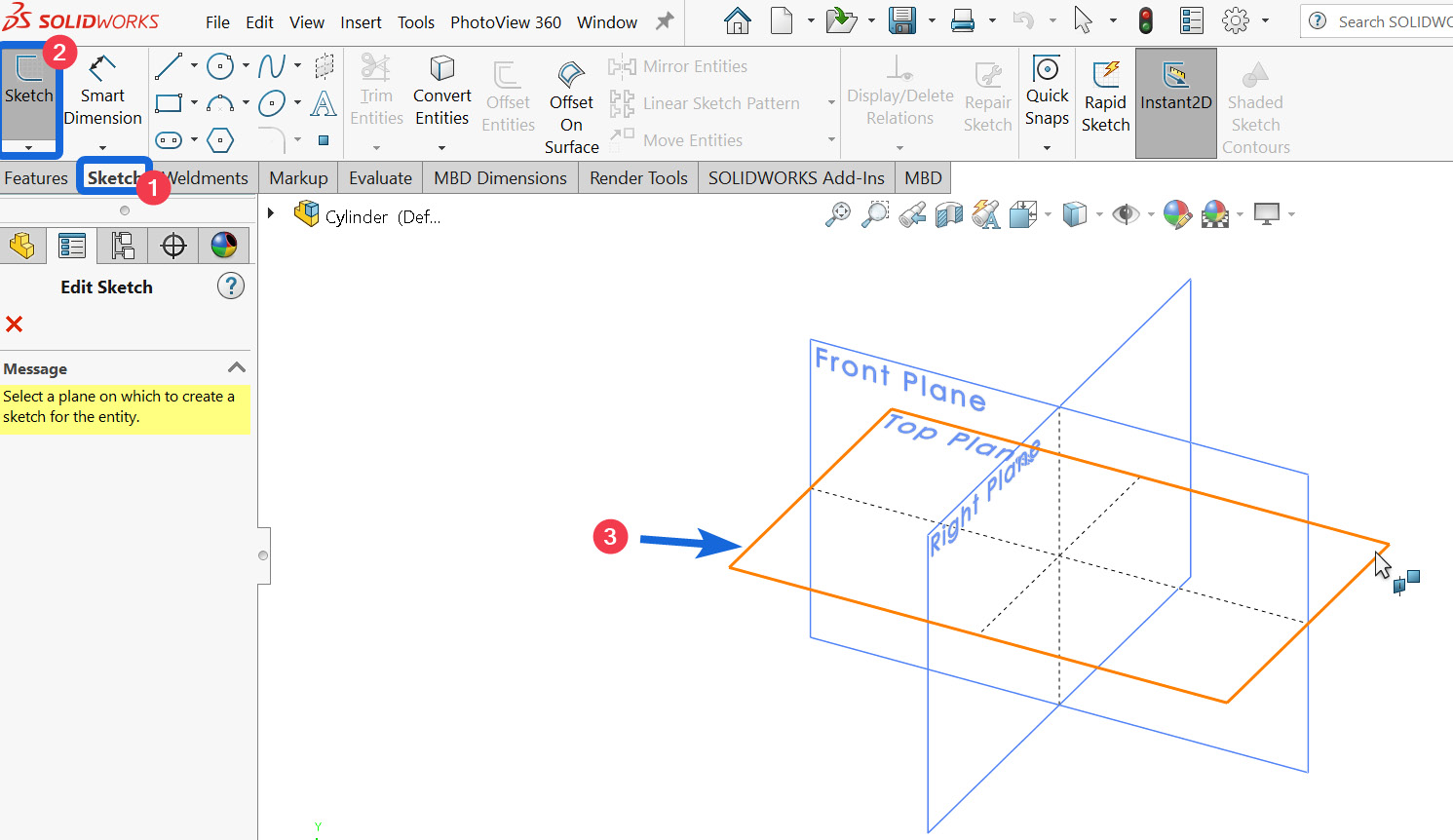
   Figure 5.5 – Choosing Top Plane

4. Use the Line sketching command to create the lines with the dimensions depicted in the following diagram.

   Ensure that the dashed line symbolizing the axis of symmetry is positioned at the origin of the coordinate system:

   

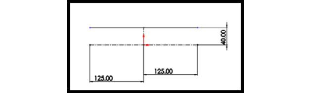
   Figure 5.6 – Axis of symmetry and the generator line for the cylindrical section

5. Create two arcs on the sides of the line shown in the following diagram by using the Centerpoint Arc command:

Figure 5.7 – Completing the profile of the vessel with the arc of the hemispherical head

Note that the profile we have created represents the outer edge of the vessel. Now that we've completed the profile, we can employ the revolve command.

Revolving the profile

The revolve command, like the extrude command we used in Chapter 4, Analyses of Torsionally Loaded Components, allows us to convert primitive line sketches into a solid body. Follow these steps to revolve the profile:

1. Navigate to the Features tab.
2. Click on Revolved Boss/Base (Figure 5.8a).
3. Upon activating the Revolved Boss/Base command, you will get the prompt window shown in Figure 5.8b. The prompt is asking if we want to close the profile.

   Select No:

   

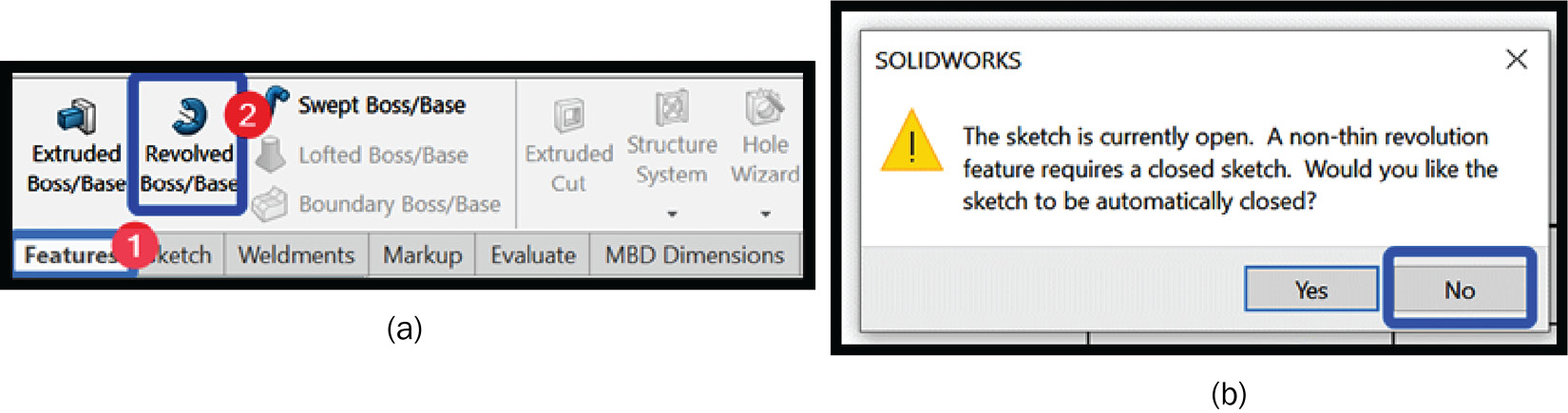
   Figure 5.8 – Activating the revolve feature

   At this point, we will see the Revolve property manager. Now, let's set some options within the Revolve property manager.

4. Under the Axis of Revolution box (labeled 1 in Figure 5.9), select the dotted centerline. Notice that the default value of the revolving angle (labeled 2) is 360.00deg. If we keep this value, a full model of the vessel will be formed, as shown in the following screenshot:
   

   Figure 5.9 – A full model of the vessel

5. Key in the value of 90deg in the revolving angle box (labeled 2 in Figure 5.10a).
6. Key in the value of 2.5mm in the thickness box (labeled 3 in Figure 5.10a).
7. Click OK (the green ).

   By completing these steps, you will get a quarter model of the vessel, as shown in Figure 5.10b:

Figure 5.10 – Options for creating the quarter symmetric model of the vessel

Caution about the Revolve Feature

A tricky issue you should be mindful of when you used the revolve feature is the direction that the thickness is added. Always ensure that the side that the thickness is applied to follows your intentions. In the preceding cases, we have accepted that the thickness is to be added inside the line because the lines we created in Figure 5.7 denote the outer wall.

It is worth pointing out that we can save even more computational resources by employing half of the quarter model we've created. If we did that, then we would have a one-eighth model, but we'll leave that as an exercise for you to try later.

Having creating the model, we are now ready to move on and convert the partial revolved body into a surface body.

Creating a surface body

You may be wondering why we need to create a surface body. The reason is that to create a shell-based mesh during the discretization process, SOLIDWORKS need a surface body. We will use the mid-surface approach of creating a surface to transform the solid revolved body into a surface body.

To this end, follow these steps to create the mid-surface body from the partially revolved body we created in the previous section:

1. Click Insert by going to Main Menu (Figure 5.11).
2. Choose Offset:
   

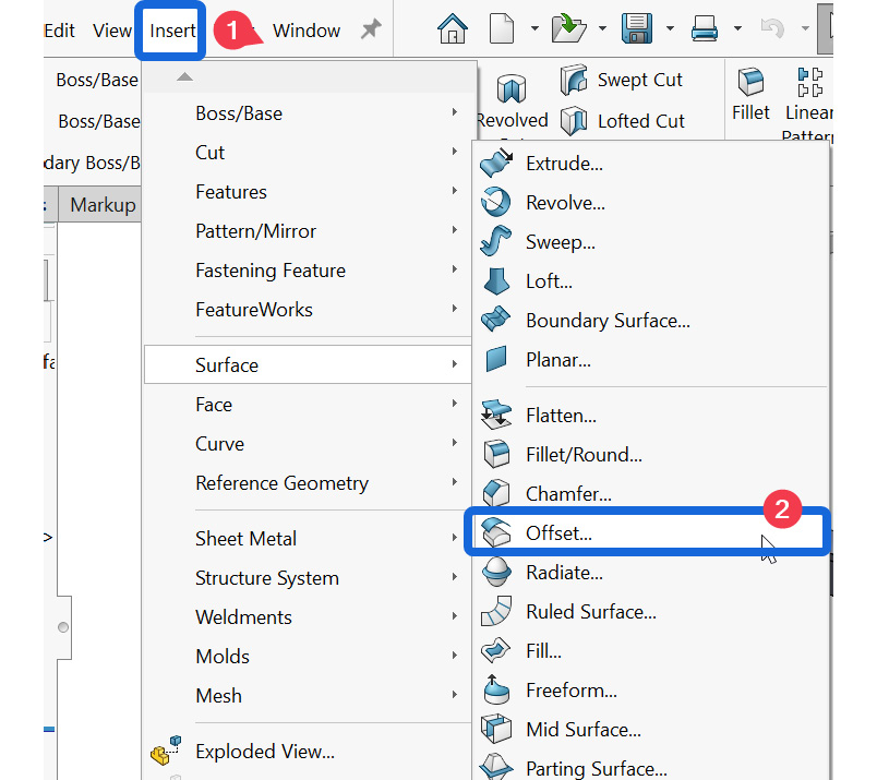
   Figure 5.11 – Activating the Offset command to create a surface

   The Offset Surface property manager will appear. Complete the necessary actions by following the following steps.

3. Click inside the Surfaces of Faces to Offset box (labeled 1 in Figure 5.12) and navigate to the graphic window to select all three inner faces.
4. Within the Offset Distance box (marked 2 in Figure 5.12), key in 1.25mm.

   If need be, click to change the direction of the offset so that the offset's surface is between the inner and outer faces.

5. Click OK:

Figure 5.12 – Converting the revolved body into a mid-surface body

We now have two bodies in the form of the mid-surface body we just created and the solid revolved body from which it is formed. The folders referring to these two bodies are highlighted in Figure 5.13a. We will delete the solid body (in a way, it is just being suppressed).

To delete the solid body, navigate to FeatureManager and follow these steps:

1. Right-click on Solid Bodies(1), as shown in Figure 5.13a.
2. Select Delete/Keep Body.
3. From the Delete/Keep Body property manager that appears, keep the options shown in Figure 5.13b.:

Figure 5.13 – Deleting the solid body

The preceding steps will produce the thin surface body shown here:

Figure 5.14 – The generated mid-surface body

Before we move on, let's add an axis that will pass through the center of the surface body. This will coincide with the axis of symmetry. Follow these steps:

1. Navigate to FeatureManager and select the Front Plane and Top Plane symbols, as shown in Figure 5.15.
2. Move to Command Manager and click on Reference Geometry (labeled 2).
3. Select Axis from the pull-down menu that appears:

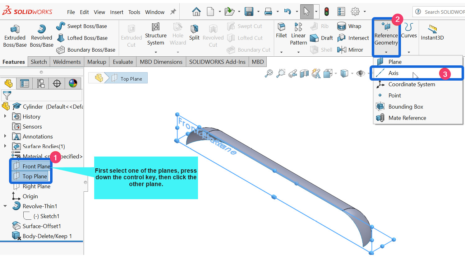
Figure 5.15 – Creating the central axis for reference

After completing step 6, the Axis property manager will appear. Keep the options within the Axis property manager as shown in Figure 5.16a. In response to the preceding actions, an axis will be created, as reflected in Figure 5.16b:

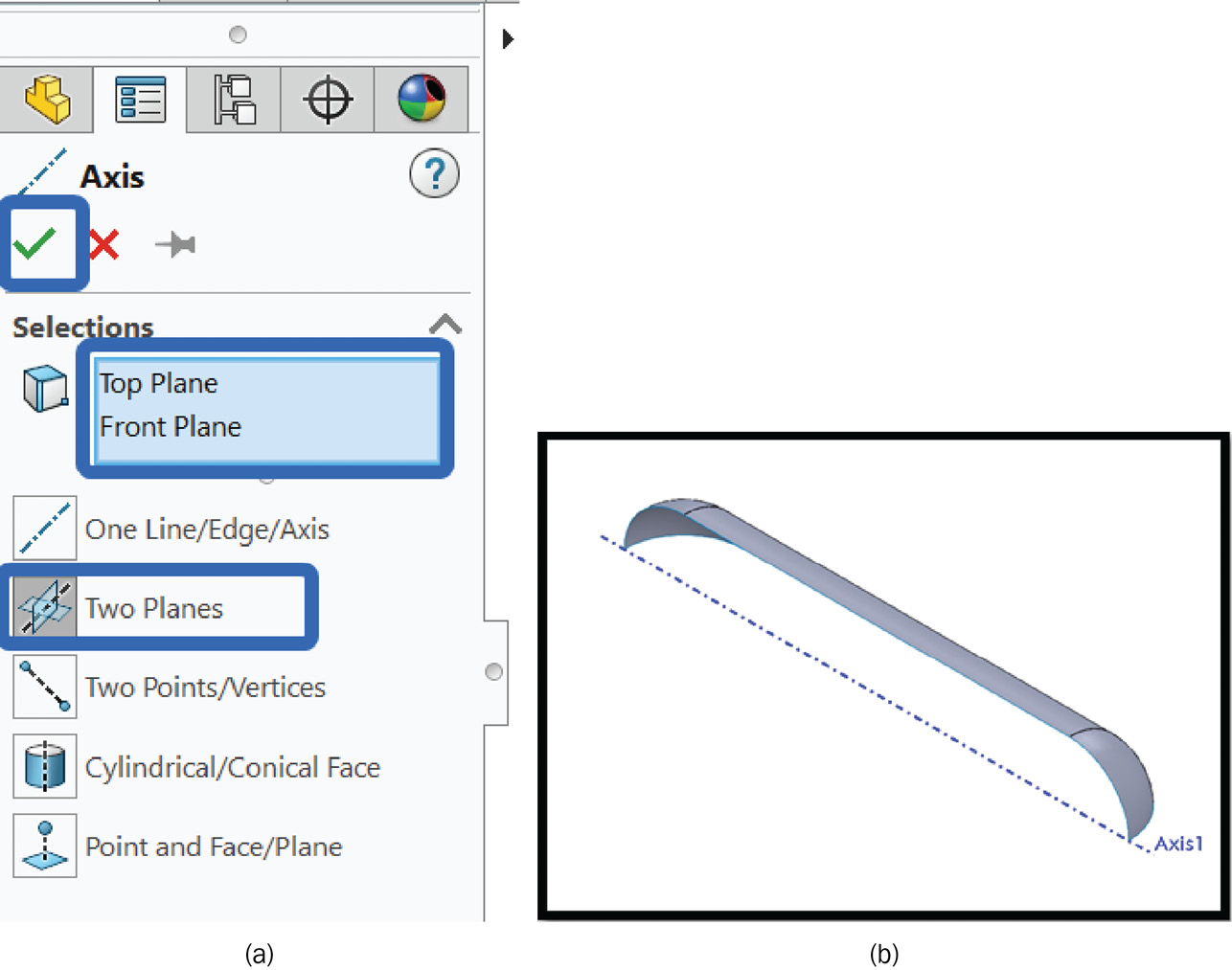
Figure 5.16 – (a) The axis property manager; (b) the created axis

At this point, we have created a mid-surface quarter model of the vessel from a partially revolved solid body. In the next subsection, we will launch the simulation study.

Part B – Creating the simulation study

This section comprises subsections that cover the usual preprocessing tasks, including activating the simulation study, assigning a material, applying a fixture, and specifying the load.

As usual, we will begin by activating the simulation environment.

Activating the simulation tab and creating a new study

To activate the simulation commands, follow these steps:

1. Click on SOLIDWORKS Add-Ins.
2. Click on SOLIDWORKS Simulation to activate the Simulation tab.
3. With the Simulation tab active, create a new study by clicking on New Study.

   Note

   The illustrative images for steps 1 – 3 are similar to what we did, for instance, in Chapter 4, Analyses of Torsionally Loaded Components, in the Part B – Creating the simulation study section. If need be, you may refer to that section for a guide.

   Within the Study property manager that appears (after completing step 3), follow these steps.

4. Input a study name within the Name box; for example, Hemi-cylinder analysis.
5. Keep the Static analysis option (selected by default).
6. Click OK.

The result of completing the preceding steps is shown in the following screenshot:

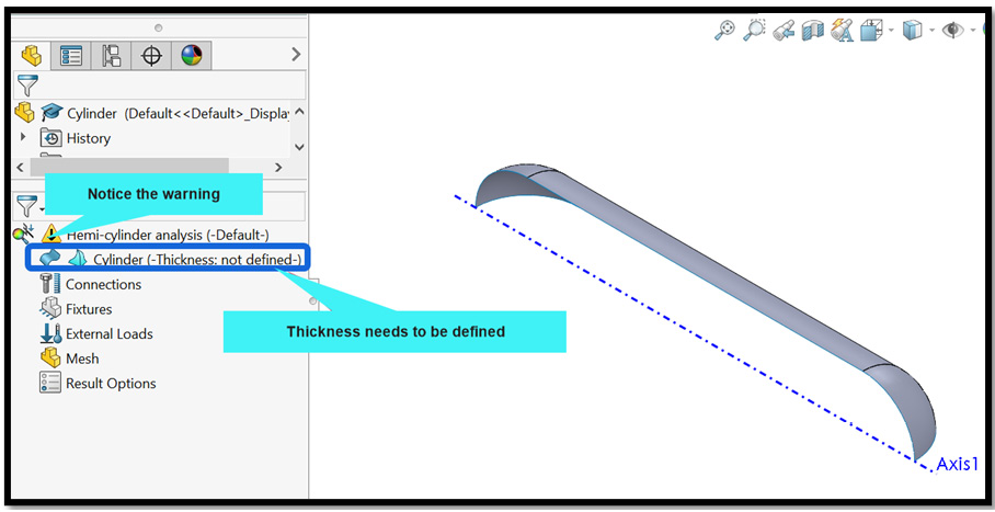
Figure 5.17 – Simulation property manager

As we can see, a warning is attached to the study name. As explained in Chapter 4, Analyses of Torsionally Loaded Components (in the Converting the extruded solid bodies into beams subsection), you can analyze a warning by right-clicking on the study name and choosing What's Wrong. If you do that, it will be disclosed that thickness is not defined for the shell body.

Therefore, our next action is to define the thickness of the surface.

Assigning thickness

Follow these steps to assign the thickness that will be used for the shell mesh:

1. Within the simulation study tree, right-click the surface body (named Cylinder (-Thickness: not defined)) and select Edit Definition, as shown in the following screenshot:
   

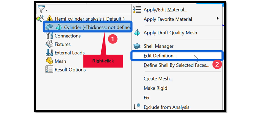
   Figure 5.18 – Assigning thickness for the shell mesh

   Within the Shell Definition property manager that appears, perform the following actions.

2. For the Type option, select Thin, as shown in Figure 5.19.
3. Within the thickness box (marked as 2), key in 2.5mm.
4. Activate the Full preview option.
5. Click OK:

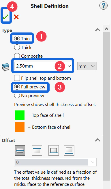
Figure 5.19 – Shell definition property manager

With that, we have defined the thickness of the surface. But notice that in addition to specifying the thickness, this step has also allowed us to select a thin shell assumption (rather than a thick shell assumption). Furthermore, once we complete the actions for defining the thickness, the warning sign attached to the study name (highlighted in Figure 5.17) will disappear.

Now, let's apply a material to the component.

Applying a material

By now, you should already be familiar with how to assign a specific material (due to what we explored in the previous three chapters). Nonetheless, the vessel is made of steel, according to the problem statement. To apply the desired material, follow these steps:

1. Right-click on the surface body and choose Apply/Edit Material.
2. Expand the Steel folder.
3. Click on AISI Type 316L stainless steel.
4. Click Apply and Close.

Note that the class of steel we have selected here (AISI Type 316L stainless steel) has Young's modulus which matches the one specified in the problem statement.

With the material assigned, our next goal is to apply the external load (internal pressure) and the specification of the fixture. Let's start by applying a fixture.

Applying a fixture

Given that we are using a partial symmetric model instead of the full model of the vessel, we need to apply symmetric boundary conditions. In this book, this is the first time that we are using this kind of boundary condition. Oftentimes, applying symmetric boundary conditions should be done with care, and there can be more than one way of doing this. For this problem, we need to apply the boundary conditions to the two major edges of the quarter model.

Follow these steps to apply symmetric boundary conditions on the edge of the quarter model that aligns with the Front Plane area.

Under the simulation study tree, do the following:

1. Right-click on Fixtures.
2. Pick Advanced Fixtures from the context menu that appears:
   

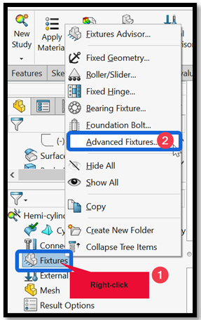
   Figure 5.20 – Choosing Advanced Fixtures

3. Within the Fixture property manager that appears, select Reference Geometry.
4. Click inside the Faces, Edges, and Vertices box (labeled 1 in Figure 5.21). Then, navigate to the graphics window and pick the three edges that align with the Front Plane area, as shown in Figure 5.21.
5. Click inside the geometry reference box (labeled 3) and select the Front Plane area:
   

   Figure 5.21 – Picking the first set of edges to apply a symmetric fixture

6. Still within the Fixture property manager, under the Translations and Rotation degrees of freedom, keep the options shown in Figure 5.22.
7. Click OK:

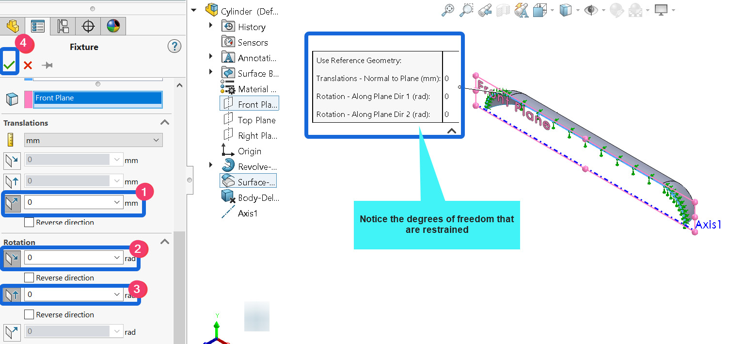
Figure 5.22 – Selecting the right combinations of movements to be restrained for the edge facing the front plane

Steps 1 – 7 covered applying the symmetric boundary conditions to the edges facing the Front Plane area.

Note about the Boundary Condition

What does the symmetric boundary condition we completed in the preceding steps imply? Well, as shown in the preceding screenshot, we have prevented the translational displacement of the edges in the direction of the Front Plane area. What we have done here is prevent translation of the edges along the Z-axis. Additionally, we have prevented the rotational displacements of the edges concerning Dir 1 (which is along the X-axis) and Dir 2 (which is along the Y-axis).

Now, we have to repeat a similar series of steps for the other symmetric edge of the model. These next set of edges align with the Top Plane area.

To apply the symmetric constraint to the other symmetric edge, move to the simulation study tree and follow these steps:

1. Right-click on Fixtures.
2. Pick Advanced Fixtures from the context menu that appears.
3. Within the Fixture property manager that appears, select Reference Geometry.
4. Click inside the Faces, Edges, and Vertices box (labeled 1 in Figure 5.23). Then, navigate to the graphics window and pick the three edges that align with the Top Plane area, as shown in Figure 5.23.
5. Click inside the geometry reference box (labeled 3) and select the Top Plane area:
   

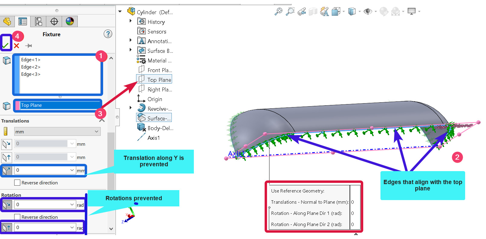
   Figure 5.23 – Picking the second set of edges to apply a symmetric fixture

6. In the Translations and Rotation degrees of freedom, keep the options reflected in the preceding screenshot.
7. Click OK.

By completing the foregoing steps, the appearance of the model in the graphics window should look as follows:

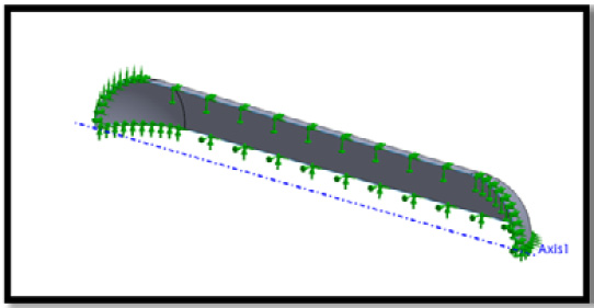
Figure 5.24 – Appearance of the model with the symmetric conditions on the two major edges

Note

When applying the boundary conditions to the edges of the model, we used the front and top planes as reference planes. Note that it is also possible to use the central axis we created earlier as a guide. While doing so will yield the same result, you should use reference planes to create an intuitive feel for the directions of the degrees of freedom we've constrained.

Now that we've applied the necessary symmetric boundary conditions, let's shift our attention to applying internal pressure.

Applying internal pressure

To apply the internal pressure on the inner face of the surface, follow these steps:

1. Right-click on External Loads and select Pressure:
   

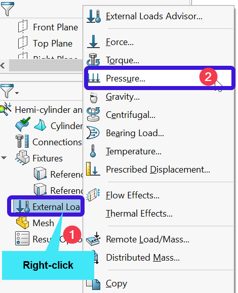
   Figure 5.25 – Applying internal pressure

   Within the Pressure property manager that appears, perform the following actions.

2. Under Type, keep the default option as Normal to selected face (labeled 1 in Figure 5.26).
3. Click inside the Faces for Pressure box (labeled 3). Then, navigate to the graphics window to pick the inner faces of the surface:
   

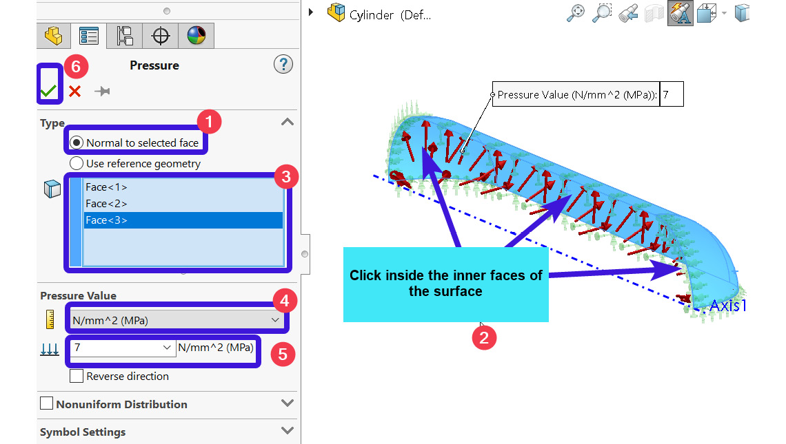
   Figure 5.26 – Options for the internal pressure application

4. Under Pressure Value, change the unit to N/mm^2 (MPa) (see the box labeled 4 in Figure 5.26).
5. Under the Pressure magnitude, input 7 (ensure that the unit system is in N/mm^2 (MPa), as specified in Step 4).
6. Click OK.

At this point, we have assigned thickness to the surface body, defined the material property, applied symmetric fixtures to the two major edges of the surface, and applied the internal pressure. It is now time to create the mesh.

Let's get to it.

Part C – Meshing

This section focuses on the discretization operation. Unlike in the previous three chapters, a standalone section has been dedicated to the meshing task for this problem. The reason for this hinges on the difference in the requirement for meshing components with shell-based elements (in contrast with the truss/beam-based elements).

You will also recall that, in the previous three chapters, we employed the concept of Mesh and Run without paying much attention to the settings of the mesh. Essentially, we exploited the concept of critical positions in those chapters, which subsequently lead to the creation of joints at critical points of the beam-like structures. Consequently, the use of critical positions eschews the need for intricate meshing operations.

However, for structures such as the pressure vessel being analyzed here, joints do not appear naturally. Simply put, these components exist as continuum structures. Consequently, the discretization of such components must be done to allow sufficient elements to be used in the analysis.

As a consequence, the general rule when using advanced elements (such as shell elements) is to pay special attention to the mesh's quality. For shell elements (and solid elements), we can experiment with the different qualitative levels of the mesh within SOLIDWORKS (for example, coarse, medium, or fine mesh). With a set of coarse meshes, we are discretizing the structure with fewer elements and thereby using fewer computational resources. In contrast, a collection of fine meshes involves a smaller number of elements. Although simulations with a finely meshed structure may take a relatively long time to run (especially for complex bodies), they produce more accurate results (assuming other aspects of the simulation workflow have been set up correctly).

In the next subsection, we will start by examining the simulation results based on the choice of a coarse mesh. Then, we will leverage a relatively fine mesh for the same problem.

We will also look at two features of SOLIDWORKS that allow a study to be duplicated and the results to be compared between different simulation studies.

Creating a coarse mesh

Begin the meshing procedure by following these steps:

1. Right-click on Mesh within the simulation study tree.
2. Select Create Mesh:
   

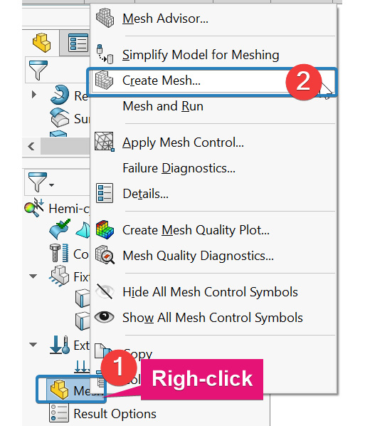
   Figure 5.27 – Initiating the meshing operation

   Once the Mesh property manager appears, you need to carry out the next steps.

3. Under Mesh Density, drag the Mesh Factor control bar (labeled 1 in Figure 5.28a) to the left.
4. Under Mesh Parameters, change the choice to Curvature-based mesh.
5. Click OK.

   Figure 5.28b shows the discretized surface body using the coarse mesh settings:

Figure 5.28 – (a) Options to create a coarse mesh; (b) The meshed surface body

Before we move on to the next action, notice that the size of the minimum triangular element (roughly 5.65 mm) highlighted in Figure 5.28b is bigger than the thickness (2.5 mm) of the pressure vessel being analyzed. In practice, the minimum element size should be a fraction of the thickness (or a fraction of the smallest non-aesthetic dimension) within the component. Nevertheless, despite the large size of the element, selecting curvature-based mesh (in step 4) and adopting the thin-walled option will facilitate relatively good results. Note that the curvature-based mesh employs the parabolic triangular mesh we discussed in the Characteristics of shell and axisymmetric plane elements subsection.

We are now set to run the analysis to obtain some preliminary results.

Running the analysis with the coarse mesh

Follow these steps to complete the running operation:

1. Right-click on the study name and select Run (Figure 5.29a).
2. You may get a suggestion about allowing the use of the Large Displacement option; select No (Figure 5.29b):

   About the Large Displacement Option

   Note that we have chosen to disregard the large displacement option in this analysis because we are running a linear analysis with a component that has linearly elastic material properties. The large displacement option is ideal for simulation tasks that involve nonlinear analysis or involve components with hyperelastic material properties such as soft polymers and elastomers et cetera.

Figure 5.29 – (a) Running the analysis; (b) Disregard suggesting to use the Large Displacement option

By running the analysis, the default solution results will be produced, as shown in the following screenshot:

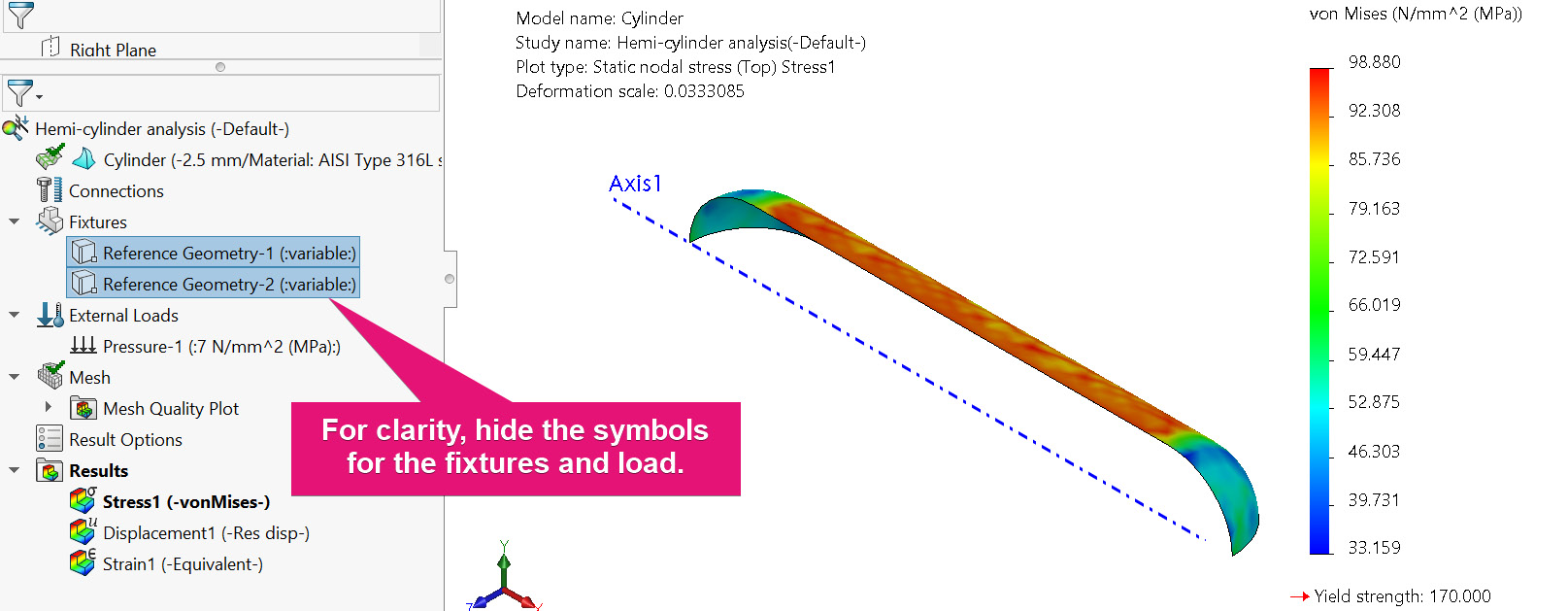
Figure 5.30 – Default results from running the analysis

As we can see, the default results include Stress 1(-vonMises-), Displacement1(-Res disp-), and Strain1(-Equivalent-). While these values are useful for general engineering assessments, our focus for this case study is the principal stresses that were developed in the cylindrical section of the vessel. Primarily, we are interested in the first and second principal stresses so that we can compare them with the analytical results. Going forward, we shall delete the displacement and strain results and then retrieve the principal stresses.

Obtaining the first principal stress

Let's start by obtaining the first principal stress by following these steps:

1. Right-click on the Results folder and select Define Stress plot.

   Now, we will work with the options within the Stress plot property manager (summarized in Figure 5.31a) that appears.

2. On the Definition tab, navigate to Display.
3. Select P1: 1st Principal Stress.
4. Within the unit box (labeled 2 in Figure 5.31a), change the unit to N/mm^2 (MPa).
5. For the Shell face option (labeled 3), select Top (this will display the result for the outer face of the surface).
6. Under Advanced Options, tick Show plot only for selected entities (this is labeled 4 in Figure 5.31a).
7. Click to activate the Select faces for the plot box (labeled 5 in Figure 5.31a). Then, navigate to the graphics window to select the outer face of the surface.
8. Now, go to the Chart Options tab. Then, under Position/Format, change the number format to floating, as depicted in Figure 5.31b.
9. Click OK:

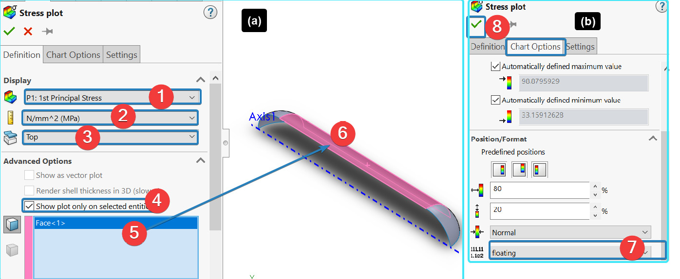
Figure 5.31 – Specifying the options for the stress plot regarding the first principal stress

With steps 1 – 9 completed, the graphics window will be updated with the plot of the first principal stress, as shown in the following screenshot. Note that the maximum value of this principal stress happens to be roughly 114.202 MPa. This maximum value is along the circumferential direction:

Figure 5.32 – Distribution of the first principal stress

Now, for us to compare the values of the first principal stress produced by the simulation with the analytical theoretical formula later, we must retrieve the average value of the principal stress that was developed within the cylindrical section. This should be a few points away from the edges that connect the cylinder to the hemispherical cap and away from the supported edges. To get the points that match this description, we will employ the Probe tool, as outlined next.

Using a probe with the first principal stress

Follow these steps to retrieve the average value of the first principal stress at specific points on the cylindrical section:

1. Right-click on Stress2 (-1st principal-).
2. Select Probe from the resulting menu:
   

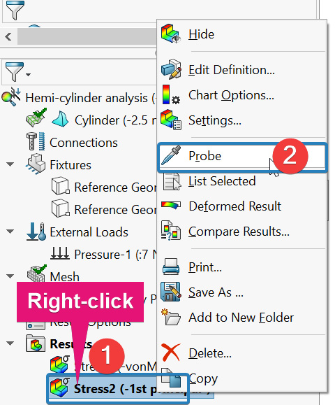
   Figure 5.33 – Selecting Probe for the first principal stress

3. Keep the options in the Probe Result property manager that are shown in the following screenshot.
4. Navigate to the graphics window and click on four random points around the center of the top face of the surface:

Figure 5.34 – Options for the Probe Result property manager and the average value of the first principal stress

A table summarizing the stress values will be displayed in the lower-left corner of the Probe Result window, as shown in the preceding screenshot. From this summary table, the average value of the first principal stress is computed to be 107.604 MPa. Recall that we obtained the maximum value of this principal stress as 114.202 MPa in Figure 5.32. We will come back to this value later. But before that, we need to obtain the second principal stress.

Obtaining the second principal stress

To obtain the second principal stress, we've got to repeat steps 1 – 9 of the Obtaining the first principal stress subsection. For brevity's sake, the following screenshot illustrates the choices that need to be made via the Stress plot property manager:

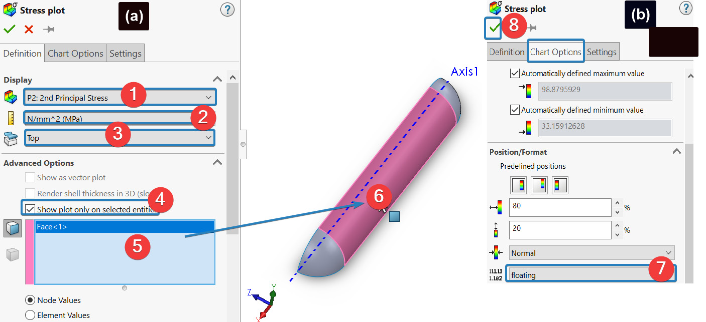
Figure 5.35 – Specifying the options for the stress plot regarding the first principal stress

Furthermore, we also need to repeat steps 1 – 4 specified in the Using a probe with the first principal stress subsection. By contextualizing the aforementioned steps for the second principal stress, you should obtain the following output:

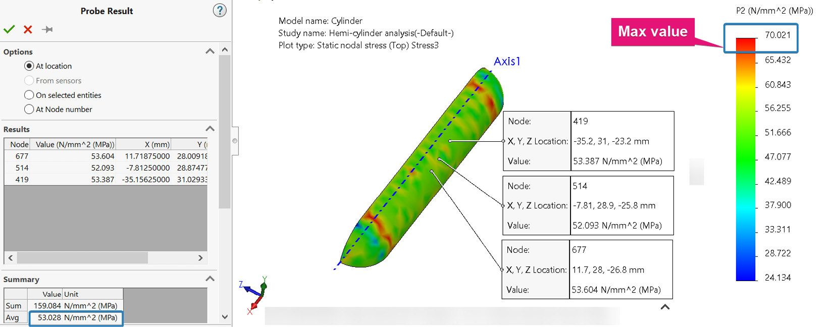
Figure 5.36 – The probed average value of the second principal stress

As we can see, the average value of the second principal stress for the cylindrical section is depicted as 53.147 MPa. However, the maximum value of the second principal stress is determined to be 70.021 MPa. The second principal stress corresponds with the axial/longitudinal stress. As a result, note that the maximum value of the second principal stress is located near the joint between the hemispherical end and the cylindrical sections.

We can now summarize the results as follows:

• The average value of the first principal stress: 107.604 MPa
• The average value of the second principal stress: 53.147 MPa
• The maximum value of the first principal stress: 114.202 MPa
• The maximum value of the second principal stress: 70.021 MPa

According to the theoretical analytical formula for the thin-walled cylindrical shell, the two major principal stresses are known to be the circumferential/hoop stress (maximum of the two) and the axial/ longitudinal stress (about half of the hoop stress).

Hearn [4] determined the values of the hoop and axial stresses for the problem as 105 MPa and 52.5 MPa, respectively. Compared to what we have just obtained from the simulation, we can conclude that the simulation result is closer to the analytical values obtained by Hearn [4].

Maximum Stress Values

Note that we used the simulation to obtain the preceding stresses and we have compared some of the values with the theoretical predictions. As you may recall, at the beginning of the case study, we stated that the effect of the support structures and opening of the vessels are neglected. If we consider these components, then the location of the maximum stress may shift to the vicinity of these discontinuities. Consequently, the principal stresses from the simulation could have differed from the theoretical calculations. One of the beauties of using finite element tools such as SOLIDWORKS simulation is being able to deal with such complicating effects with ease. Simulation tools allow us to go beyond what we can do with hand calculations!

So far, we have produced results by using a coarse mesh. Now, let's improve the mesh's quality and see what happens to the maximum values of the two principal stresses. We will do this briefly in the next subsection.

You are encouraged to save the analysis file, but do not close the file yet.

Employing a finer discretization

Now, to employ finer mesh elements to rerun the analysis, we will duplicate the study we have completed using the coarse mesh. Doing so will help us build on the settings we have implemented previously, and thus save us from having to start from scratch.

To duplicate the study, follow these steps:

1. Navigate to the base of the graphics window and right-click on the study tab (named Hemi-cylinder Analysis).
2. Select Copy Study.
3. Within the Copy Study property manager that appears, provide a name for the new study such as Fine Mesh Analysis, as indicated in Figure 5.37b.
4. Click OK:

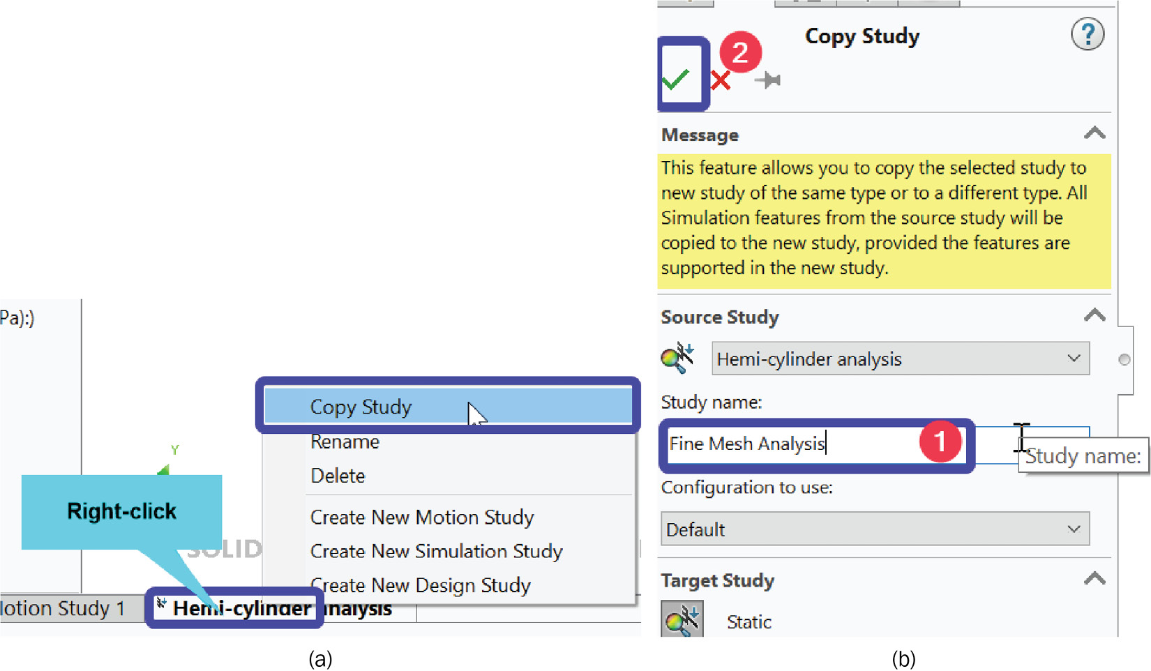
Figure 5-37 – (a) Duplicating the completed study; (b) Copy Study options

After completing steps 1 – 4, a new study tab will be launched beside the old study tab. Ensure you remain in this new study environment.

To refine the mesh, use the Create Mesh option (for a guide on this, refer to Figure 5.27) to generate a new mesh setting. Simply drag the Mesh Factor button toward the right, as shown in Figure 5.38a. The resulting meshed body, with a finer set of elements, should be similar to what we have in Figure 5.38b:

Figure 5.38 – Creating a finer mesh

Note

Any time you try to create a new mesh inside a duplicated study environment, you will likely get a warning stating that Remeshing will delete the results for the study. Since the results of the simulation with the fine mesh need to be updated, you should simply accept the warning by clicking OK.

Having refined the mesh, you can now run the analysis again (for a guide, refer to the Running the analysis with a coarse mesh subsection). Once we've done this, we will have a new set of results. Therefore, we are now in a state to compare the results.

Comparing the results

One of the useful features of the SOLIDWORKS simulation is the ease with which the results of different studies can be compared. To exploit this feature to compare the results of the analyses conducted with the finer mesh and the one conducted with the coarse mesh, follow these steps:

1. Right-click on the Results folder in the current study tab.
2. Select Compare Results (Figure 5-39a).
3. Within the Compare Results property window that appears, under Options, tick the All studies in this configuration box (this action reveals all the available studies in the configuration).
4. To compare the values of the two principal stresses from the two studies, make the selection depicted for the box labeled 2 in Figure 5.39b:

Figure 5.39 – Initiating the process of comparing the results

Upon completing the preceding actions, the graphics window will be updated and four windows corresponding to the four principal stresses will be displayed, as shown in the following screenshot:

Figure 5.40 – Four windows showing the selected results for the two studies

As you can see, the maximum value of the first principal stress has reduced to 113.382 MPa (which is roughly 5.4% closer to the theoretical prediction), while the minimum value of the second principal stress has increased to 51.532 MPa (roughly about 3.4% of the value of the second principal stress). Further, you will notice that there is a smooth variation in the color of the stress distribution for the results obtained using the fine mesh, indicating much better convergence of the results.

For this simple problem, the effect of refining the mesh may not appear to be significant, but for a large assembly of components, analysts must carry out convergence analysis to determine how changes in mesh quality affect a specific result of interest (usually stress or displacements in static analysis) and to determine an acceptable element size. The reason for this is that, oftentimes, for a large assembly with multiple components, using a coarse mesh may not always give an accurate result, while using an ultra-fine mesh will incur a costly simulation duration. So, a compromise is needed to strike a good balance between mesh quality, the desired result accuracy, and simulation duration. We will explore convergence analysis in more detail in Chapter 10, A Guide to Meshing in SOLIDWORKS.

We hope this section has given you a taste of what effect the mesh's quality can have when using advanced elements such as shell elements. At this point, it is worth pointing out that although we have focused our attention on the principal stresses, you can pretty much retrieve other results of interest. For instance, we could have also used the value of the von Mises stress to determine if the vessel will fail or not. We could have also used the value of the resultant displacements to determine if the pressure vessel experiences excessive deformation. All these are left for you to explore.

This concludes the simulation of the first case study. This specific case study has taken us on a journey that has seen us using the shell element, applying symmetric boundary conditions, creating and refining shell meshes, and comparing results across two studies.

Now, because we will not be returning to the topic of axisymmetric body problems again in future chapters, you may want to explore one more case study, even if briefly, that will not be based on the use of shell elements.

Plane analysis of axisymmetric bodies

The approach that was adopted in the previous case study involved a thin-walled pressure vessel, for which the use of shell elements is more suitable. However, there are a variety of axisymmetric problems that involve engineering components with substantial thickness. In such cases, the use of thin shell elements may not be the best choice. This section relates to one such case.

Problem statement – case study 2

Let's start with a bit of background for the case study. In power presses, automobile engines, and a wide variety of power generation/transmission systems, mechanical flywheels are used as part of the energy storage system to smoothen out power delivery [6]. Indeed, recently, the design of the flywheel has taken a central position with the recent shift in consciousness to the demand for renewable energy. In its most basic form, a flywheel unit consists of a shaft and a solid rotating disk acting as the rotor (see Figure 5.41). One potential source of concern in the design of a flywheel energy storage system is the failure of the rotating disk due to high speed:

Figure 5.41 – Flywheel unit for electrical energy storage (see Amiryar and Pullen [7])

In this case study, we will assess the von Mises stress as well as the radial and tangential stresses that develop in a flywheel disk rotating with a mid-range speed of 20,000 rpm. Figure 5.42a shows a typical flywheel disk with a partial view of the power transmitting shaft. A sectioned view of the disk is shown in Figure 5.42b:

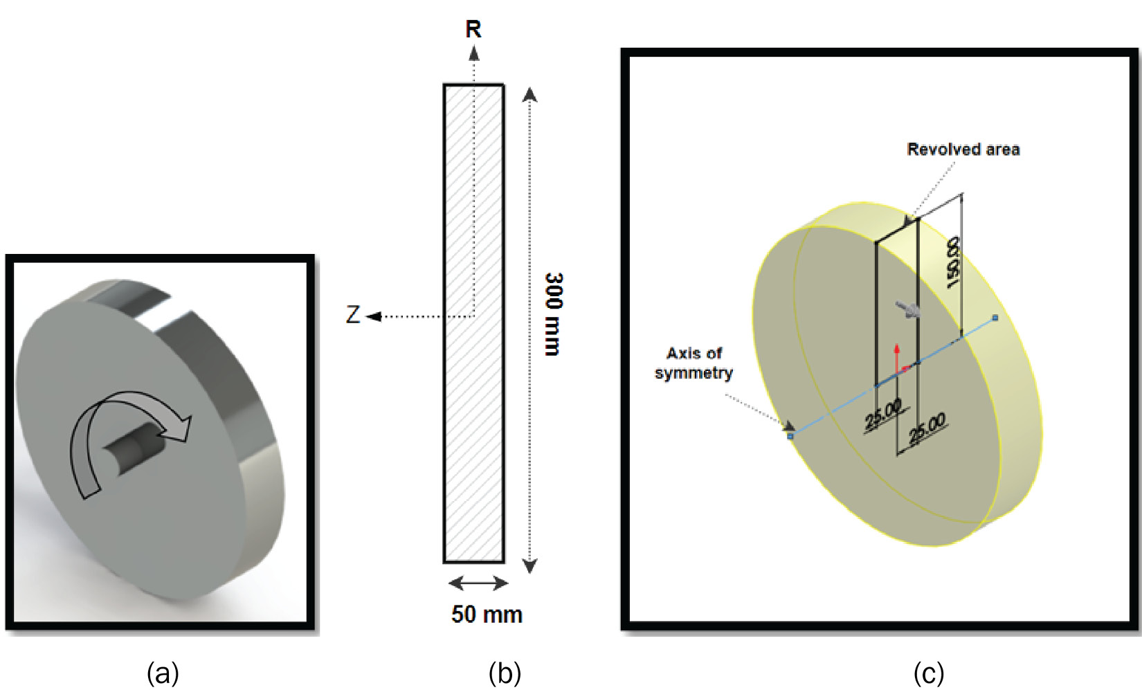
Figure 5.42 – (a) Flywheel rotor; (b) The right plane sectioned view; (c) A simplified rotating disk showing the revolved area

However, for us to compare the value of the stress obtained from our simulation with the analytical solutions for the radial and tangential stresses of a solid rotating disk, we will suppress the effect of the protruded shaft and concentrate on the disk, as shown in Figure 5.42c. Meanwhile, also shown in Figure 5.42c is the plane rectangular area that may be revolved to form the flywheel. The flywheel is made of steel with Young's modulus of 200 GPa and a Poisson's ratio of 0.3.

A brief guide to the simulation of this problem is given next.

Modeling the flywheel

In principle, there are a few ways to solve this problem using the finite element method:

• Use a simplified revolved plane section.
• Use a partial symmetric solid model, which will exploit the rotational symmetry of the problem.
• Use the full solid model of the solid disk.

The latter two approaches will require the use of solid elements, which will be covered in Chapter 6, Analyses of Components with Solid Elements. So, for now, we shall go with the approach of using the simplified revolved plane section.

A compressed set of steps to create the model are as follows:

1. Create a model of the rectangle that serves as the revolved plane on the Right Plane area (Figure 5.43a).
2. Convert the area into a planar surface by going to Insert  Surface  Planar (Figure 5.43b).
3. Add an axis to the base of the surface by going to Reference Geometry  Axis (Figure 5.43c):

Figure 5.43 – Creating the planar surface

Later in the simulation environment, we will want to apply boundary conditions to stabilize the finite element model. For this, we need to use a vertex at the middle of the edge at the base of the surface. As-is, the created surface has only four vertices at the corners. One way to create a vertex at the middle base edge of the surface is to use the Split tool. Follow these steps to split the surface:

1. Navigate to the Main Menu pulldown, select Insert  Features  Split.
2. In the Split property manager that appears, click inside the Trim Tools box (labeled 1 in Figure 5.44). Then, move to the feature manager tree to select the Front Plane area.
3. Click Cut Part.
4. Under Resulting Bodies, tick inside the boxes, as shown in the box labeled 3 in Figure 5.44.
5. Click OK:

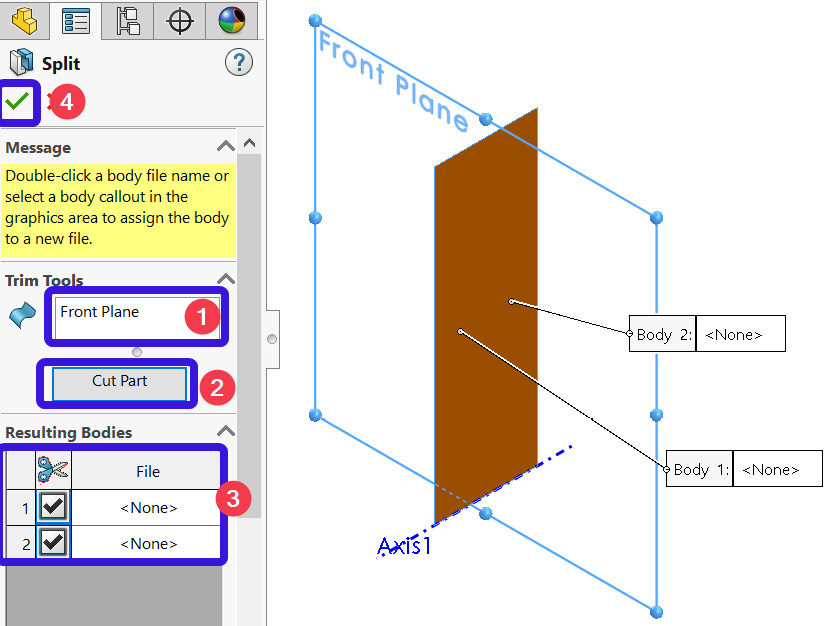
Figure 5.44 – Actions to split the surface

Once you've completed steps 1 – 5, a symbol representing that the body has been split should appear in the feature manager, as indicated in Figure 5.45. Notice the presence of the vertex in the model:

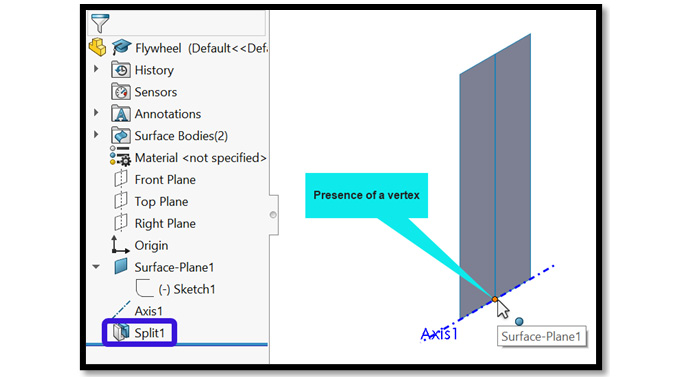
Figure 5.45 – Presence of the split bodies and a vertex

Now, our model is ready for simulation, which is what we will shift our attention to next.

Simulating the flywheel

The steps to create a new study based on 2D simplification are different from what you have seen previously. For this purpose, carefully follow these steps:

1. Using the Simulation tab, launch a New Study.
2. From the Study property manager that opens, provide a name for the study, such as Flywheel Plane Analysis.
3. Tick the Use 2D Simplification box, as shown in Figure 5.46a.
4. Click OK.

   Now, unlike all the previous studies/analyses we have conducted so far, by clicking OK another window – the 2D Simplification property manager – will open. This will allow us to pick the right type of planar simplification we wish to deploy.

5. Within the 2D Simplification property manager, under Study Type, choose Axi-symmetric (see Figure 5.46b):
   

   Figure 5.46 – Selecting the options for a 2D plane axisymmetric analysis

6. Under Section Definition, choose the Right Plane area from the feature manager.
7. For Axis of Symmetry (labeled 3 in Figure 5.46b), choose Axis1.
8. Click OK.

Note we have selected the Right Plane area in step 6 because we created the revolved area on this plane. Upon completing steps 1 – 8, we will get the now-familiar simulation study tree shown in the following screenshot:

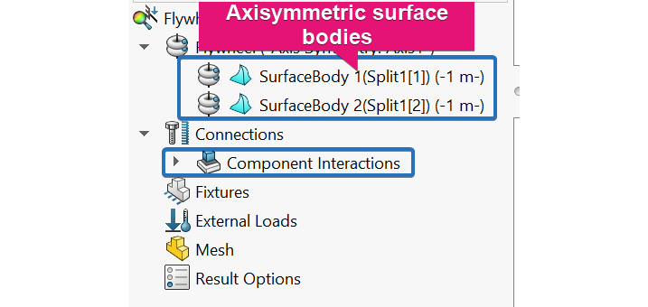
Figure 5.47 – Simulation study tree for planar analysis

Note the symbol attached to the surface body in the preceding screenshot. You will also notice the presence of the Component Interactions. This arises because of the splitting operation we performed earlier.

Now that we have arrived at the simulation environment, it is time to assign a material property, apply a fixture, apply the external load in the form of a rotational speed, create the mesh, and run the analysis. This is summarized here:

1. For the material, assign AISI Type 316L stainless steel (for a guide on this, refer to the Applying a material subsection for case study 1).
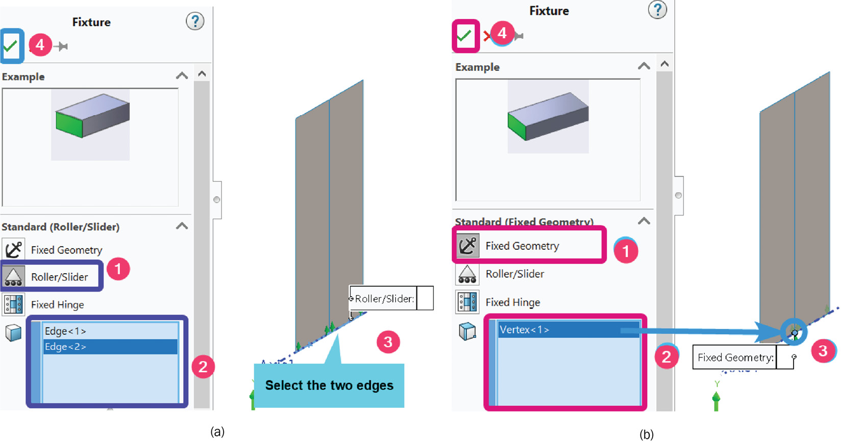
2. To apply the fixture, begin as we did in the Applying a fixture section. Using those steps, specify a Roller/Slider support on the edge at the base and use the options shown in Figure 5.48a:
   

   Figure 5.48 – Options for the fixtures

3. For the load application (centrifugal speed), follow the steps illustrated in Figure 5.49:
   

   Figure 5.49 – (a) Activating centrifugal speed; (b) Specifying the direction and magnitude of the centrifugal speed

4. To create the mesh, follow the steps outlined in the Creating a coarse mesh subsection. However, instead of using a coarse mesh, let the Mesh Factor button be in the middle. This will create a mesh of medium quality that should be satisfactory.

   At this point, the simulation study tree, together with the meshed body in the graphics area, should appear as follows:

   

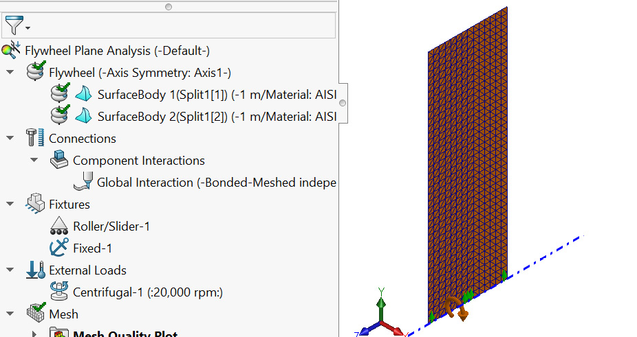
   Figure 5.50 – The updated simulation study tree and the mesh's planar body

5. Run the analysis (right-click on the name of the analysis and choose Run).

By completing all the actions outlined in steps 1 – 5, we are in a position to explore the results,.

Extracting the principal stresses in the flywheel

For validation purposes, we will extract the first two principal stresses. But before we obtain these results, let's estimate the expected value of the radial and the tangential stresses that will develop in the disk, as predicted by the following theoretical formula (see Barber [8]):

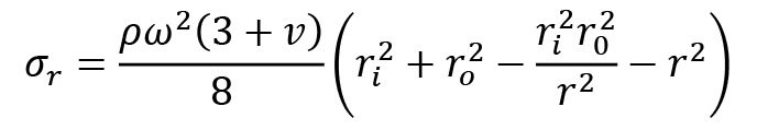(5.1)

(5.2)

Here, is a varying radial distance, while and denote the external and internal diameters, respectively. Furthermore, , , and symbolize density, Poisson's ratio, and angular velocity, respectively. From the problem statement and the material property values from the SOLIDWORKS library, we get the following formula:

Using these values, we can determine the stresses as follows:

(5.3)

(5.4)

By obtaining the principal stresses (previously illustrated and discussed for case study 1), you can compare the results from the simulation with the stress values we obtained from the analytical formula. The following screenshot shows the two principal stresses from the simulation:

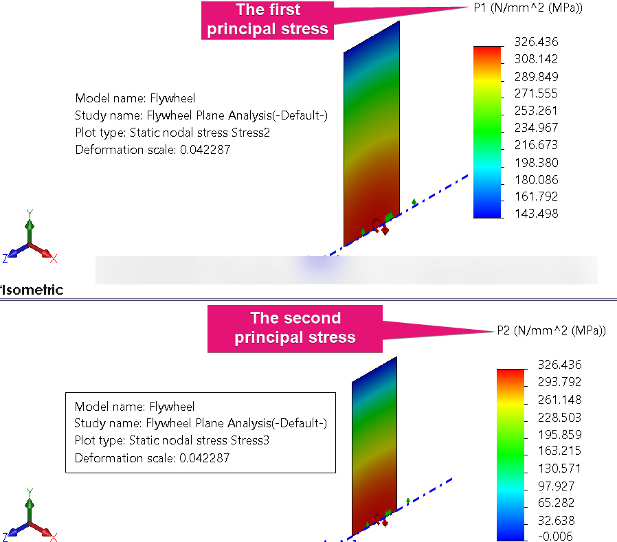
Figure 5.51 – Comparison of the principal stresses for the flywheel

As you can see, we have obtained a value of 326.436 MPa for P1 (the upper screenshot) which denotes the first principal stress, and the same value for P2 (the lower screenshot in Figure 5.51). You will recognize that a negligibly small difference exists between the computed results we have obtained from the SOLIDWORKS simulation and the prediction from the analytical expressions. This has happened despite the fact we have used fewer axisymmetric plane elements compared to what we would have used if we had conducted the analysis using the whole three-dimensional model of the flywheel disk.

The last result we will look at is the von Mises stress, which is often used as an indicator to determine the survival of the component under the applied speed. In retrieving the value for the von Mises stress, we will also show another interesting aspect of the stress plot property when using the axisymmetric plane elements, which is obtaining a 3D stress plot to perform an analysis with the axisymmetric plane elements.

Recall that the von Mises result is part of the default solution that is available under the Results folder. Consequently, what we need to do is simply edit the settings of the computed von Mises stress to obtain the 3D plot of its variation. For this purpose, follow these steps:

1. In the Results folder, right-click on Stress 1 (-von-Mises-) and choose Edit Definition (Figure 5.52a).
2. Within the Stress plot property manager that appears, choose the options indicated in Figure 5.52b. Ensure that you tick the Show 3D plot box (labeled 3). You can also specify any desired value in the angle box (labeled 4).
3. Click OK:

Figure 5.52 – (a) Editing the plot of the von-Mises stress; (b) Ways to obtain a 3D plot of the von-Mises stress

Upon completing steps 1 – 3, the graphics window will be updated to display the variation of the von Mises stress, as depicted in the following screenshot. Here, both the maximum von Mises stress and the Yield strength property of the material of the disk are highlighted:

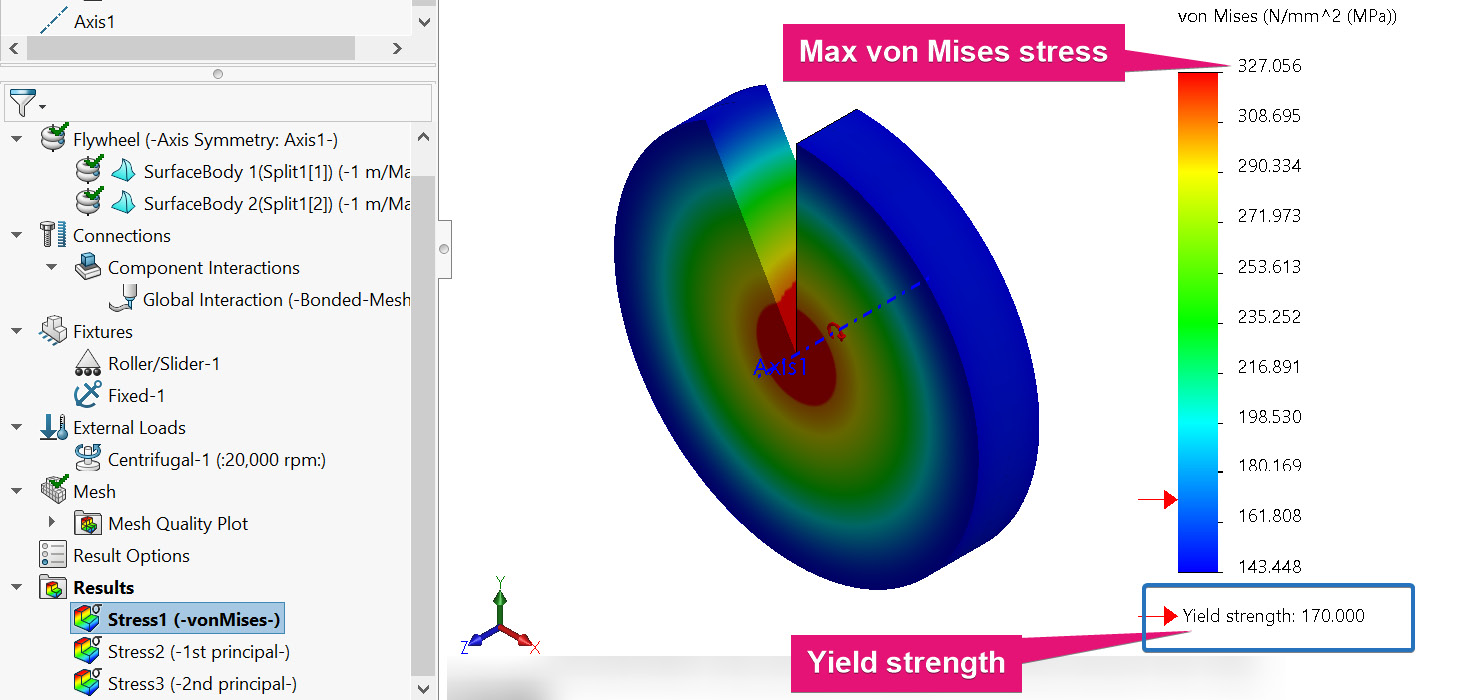
Figure 5.53 – The 3D plot of the von-Mises stress

The preceding screenshot indicates that the maximum von Mises stress is way beyond the Yield strength property of the disk. This shows that the disk will not survive the operating speed of 20,000 rpm that has been applied to it during operation. To improve this design, you may wish to change the material increase the thickness of the disk. Alternatively, if you are dealing with a design task for which the material specification is fixed, then an optimization task can be conducted to determine the optimal thickness that will allow the disk to operate safely.

With that, we can conclude this second case study. You will agree that we have come a long way. We started by providing some background details about three-dimensional bodies that are endowed with axisymmetric properties. We then walked through our first case study, which dealt with the static analysis of a thin-walled cylinder using shell elements. Following that, we took on the second case study and explored the use of the plane axisymmetric element to analyze a flywheel idealized as a rotating disk. Note that although we have deployed shell elements in this chapter solely for analyzing axisymmetric problems, their usage goes far beyond this. For instance, they can be used to analyze various forms of non-axisymmetric, thin-walled structural members.

Analysis of thick-walled cylinders

The method of using plane axisymmetric plane elements that we have exploited for the flywheel case study can also be used to conduct a planar analysis of thick-walled cylinders. But in most practical simulation problems, solid elements may be more ideal for analyzing thick-walled cylinders.

Summary

In this chapter, we explored the procedures involved in analyzing axisymmetric bodies. Various strategies for analyzing components that satisfy the axisymmetric condition were highlighted. Using two case studies, we have demonstrated how to analyze axisymmetric components with shell elements (thin-walled members) and with the axisymmetric plane element. A few of the key concepts we explored included:

• How to apply symmetric boundary conditions to the edges of partial symmetric surface body
• How to apply a pressure load and centrifugal speed load
• How to duplicate a study and how to create/refine the simulation mesh
• How to compare results between studies in the same configuration
• How to use the probe tool to obtain the average values of stress
• How to visualize a 3D plot for a study conducted with an axisymmetric plane element

You can deploy these concepts for similar design problems that you may have. In the next chapter, you will learn about how to analyze components with solid elements.

Exercises

1. A thin-walled cylindrical vessel that's 3 meters in length has an internal diameter of 1 meter and a thickness of 30 mm. The cylindrical vessel is made of AISI Type 316L stainless steel and it will contain a fluid pressure of 2.1 MPa. Create a quarter model of the cylinder and use the SOLIDWORKS simulation to determine the hoop and axial stresses in the cylinder.
2. An aircraft cabin window has been designed in the form of a thin circular plate with a radius of 600 mm and a thickness of 20 mm. The material of the window is polycarbonate with Young's modulus of 13.5 MPa and a Poisson's ratio of 0.36. Create a full model of the plate and analyze its maximum deflection and maximum principal stress using shell elements.
3. Reconduct case study 2 for a disk that has the same diameter but with a thickness of 100 mm. Use SOLIDWORKS to determine the factor of safety for the new disk under the same operating speed of 20,000 rpm and the same material property.

Further reading

• [1] Advanced Topics in Finite Element Analysis of Structures: With Mathematica and MATLAB Computations, M. A. Bhatti, Wiley, 2006.
• [2] The Finite Element Method: The basis, O. C. Zienkiewicz, R. L. Taylor, R. L. Taylor, and R. L. Taylor, Butterworth-Heinemann, 2000.
• [3] Finite Element Method with Applications in Engineering, Y. M. Desai, Dorling Kindersley, 2011.
• [4] Mechanics of Materials Volume 1: An Introduction to the Mechanics of Elastic and Plastic Deformation of Solids and Structural Materials, E. J. Hearn, Elsevier Science, 1997.
• [5] Pressure Vessel Design, D. Annaratone, Springer Berlin Heidelberg, 2007.
• [6] Power system energy storage technologies, P. Breeze, Academic Press, 2018.
• [7] A review of flywheel energy storage system technologies and their applications, M. E. Amiryar and K. R. Pullen, Applied Sciences, Vol. 7, no. 3, p. 286, 2017.
• [8] Intermediate Mechanics of Materials, J. R. Barber, Springer Netherlands, 2010.