
Chapter 1: Getting Started with Finite Element Simulation
This chapter lays the groundwork for what is to come in the later chapters. It gives a high-level discussion of the finite element method (FEM), tracing its historical origin, emphasizing its application, and outlining its implementations. Some of the key concepts regarding FEM (such as discretization, types of elements in FEM, nodes, and more) are briefly highlighted, and a snapshot of the SOLIDWORKS Simulation interface, license, and computing requirements are discussed. To this end, this chapter covers the following major topics:
- An overview of finite element simulation
- Understanding SOLIDWORKS Simulation
- Getting started with the SOLIDWORKS interfaces
- What is new in SOLIDWORKS Simulation 2021–2022?
Technical requirements
You will need to have access to SOLIDWORKS software with a SOLIDWORKS Simulation license.
You can find the supporting files for this chapter here: https://github.com/PacktPublishing/Practical-Finite-Element-Simulations-with-SOLIDWORKS-2022/tree/main/Chapter01
An overview of finite element simulation
This section offers a short account of the historical origin, importance, application, and implementation of finite element simulation.
Background
The pervasiveness of computer-aided engineering (CAE) has grown in parallel with the progress in the development of digital computers. Historically, CAE was predominantly used for the solid and surface modeling of engineering parts and assembly. However, in recent years, a glaring inroad of this progress has manifested in the simulation of various forms of engineering systems. Indeed, simulation is at the heart of the progress for advanced product development across different industries. Specifically, in the area of engineering product development, finite element simulation, which is based on the rich theoretical framework provided by the finite element analysis (FEA), represents a crucial toolkit for the following:
- A smarter and efficient design of engineering systems throughout the product development life cycle
- Minimizing product recall through rigorous analyses and examinations of the fidelity of product performance
- Facilitating iterations of virtual prototypes before incurring the cost of building physical prototypes
Information
Simulation is a word that has many definitions. Its use in this book orients toward its definition as the representation of a real physical system with a virtual prototype to study, analyze, and predict its response under external effects.
These days, FEM can be regarded as a standalone subfield of activity within the larger CAE. However, historical records place its root in the field of applied mathematics. The first documented application of the method is linked to the technical attempt to solve design problems from the aerospace industry in the 1950s. Nonetheless, the method rose to fame in the 1960s with the work of Clough [1] (please refer to the Further reading section) and the publication of the first book on FEA by Zienkiewicz and Cheung [2]. Since these events, FEM has recorded many successes, and there has been an upswing of applications spreading from the automotive, aerospace, biomedical, civil, consumer products, nuclear, and mechanical fields, to the space industry.
FEA entails transforming physical processes/products into some approximate mathematical equivalents called mathematical models. Afterward, the models are solved with appropriate computing resources via numerical solution algorithms. Now, the notion of approximation here might evoke a feeling of inferiority of finite element simulation. However, it does not in any way detract from the excellent accomplishments of FEA, some of which will be demonstrated in this book. By the virtue of their complexities, most physical objects or practical products cannot be reduced to perfect mathematical models. As a result, the process of approximation has become a time-honored trade-off that engineers have accepted and should be willing to interrogate its consequence. Viewed through this lens, being aware of the approximate nature of simulation requires analysts to be mindful of errors that arise from simulation and others closely linked with using finite element simulation software as an engine of inquiry to analyze and predict the behavior of physical entities. Nonetheless, we will explore methods of minimizing errors in finite element simulations (through convergence analysis, verification, and validation) in subsequent chapters of this book.
Meanwhile, as a subset of the CAE skills, finite element simulation was once delegated to specialists within engineering firms. However, as the line between engineering analysts and designers blurs with the proliferation of software such as SOLIDWORKS, many engineers are now required to be both familiar and proficient with complex engineering analyses related to the performance evaluations of products. It is hoped that this book serves you in the journey to acquire proficiency in this regard or will, at the very least, point you in this direction.
Applications of FEA
Although FEA gained tremendous traction from its attempts to solve the problems of structural mechanics, today, the successful applications of the methods span numerous subfields of engineering, ranging from flow analysis to thermal, electric, and magnetic fields. A non-exhaustive list of domains of the applications of FEA are presented in Table 1-1:
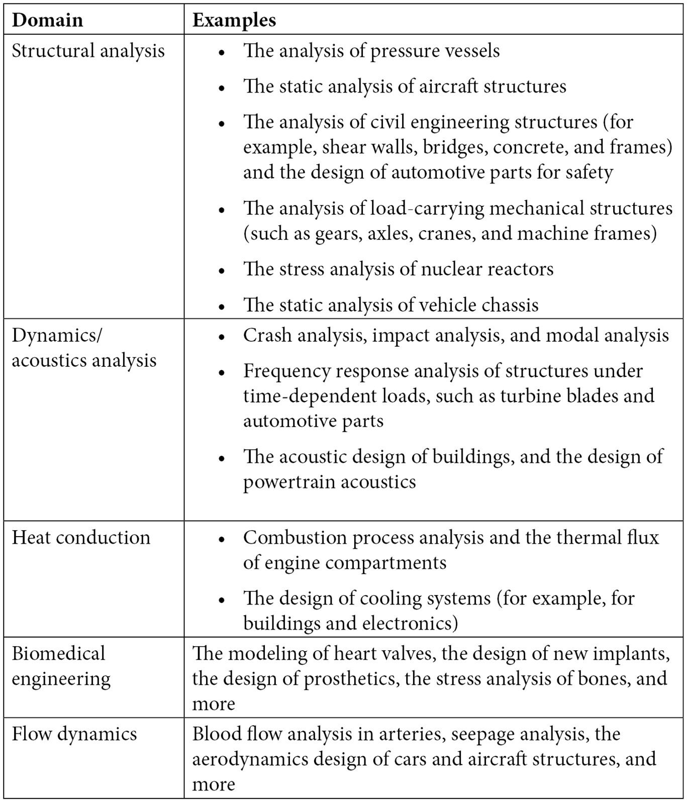
Table 1-1: Domains of applications
Implementations of FEA
Meanwhile, for simple problems, the FEA can be coded in almost any programming language. However, such programs are usually limited in scope and are often less useful for engineers dealing with the performance analysis of complex parts or assemblies. As a consequence, there are many commercial implementations of FEA.
Two categories of FEA-related software have emerged from the implementation by various corporations and entities:
- Analysis-oriented FEA software
- Design-oriented FEA software
The first category encompasses commercial implementations of FEM such as ABAQUS, ADINA, DEFORM, ANSYS, MSC NASTRAN, and COMSOL, among others. Each piece of software in this category predominantly exists as an analysts' tool. They have a comprehensive set of libraries and elements for the advanced analysis of multiphysics engineering systems. However, they tend to have a rather steep learning curve. In contrast, the software in the second category, under which SOLIDWORKS Simulation belongs, is principally developed for three-dimensional (3D) CAD modeling. However, they offer simulation suites that can be used for various analyses using the FEM. Due to the close integration between the modeling and analysis environments, the latter category generally does the following:
- It facilitates faster learning of the intricacies of FEA.
- It has a familiar and less intimidating interface for beginners.
- It has a relatively shallow learning curve for most engineers that are already familiar with the modeling interface.
Nevertheless, there are elements of overlap in both categories. For instance, a majority of the specialist FEA applications in the second category are also conferred with CAD interface for part modeling. Moreover, all implementations of FEM conceptually follow and require these three phases for product simulations:
- A preprocessing phase
- A solution phase
- A postprocessing phase
The preprocessing phase involves idealization (which translates to the transformation from a physical world to a computational domain), model generation (that is, defining the geometric domain), mesh generation (that is, creating elements and nodes), and the supplying of input data (for example, material properties, loads, and physical constraints).
In the solution phase, the governing algebraic equation in matrix form that maps to the behavior of the computational domain is solved using a numerical method. For this phase to happen, the application software will often require the user to provide details (specifically, sufficient boundary conditions) that ensure the satisfaction of compatibility and equilibrium conditions.
The postprocessing phase involves evaluations and interpretations of the computed solutions generated by the simulation and possibly an examination of the correctness. In specific terms, activities that fall under this phase encompass things such as the plotting of results, the retrieving of deformed shapes, the examination of critically-stressed areas within the components, and more.
Now that we have covered the background, applications, and some of the basic steps necessary for general finite element analyses, we will move on to introduce the SOLIDWORKS simulation.
Overview of SOLIDWORKS simulation
This section introduces the SOLIDWORKS Simulation, highlights the basic steps required for most simulations, discusses the type of finite elements provided by SOLIDWORKS Simulation, and covers the SOLIDWORKS Simulation license, its computing requirements, and its limitations.
What is SOLIDWORKS Simulation?
SOLIDWORKS Simulation is the implementation of the FEM in the SOLIDWORKS CAD environment by SOLIDWORKS Corporation (whose parent company, Dassault Systèmes, makes the SOLIDWORKS CAD software). The SOLIDWORKS CAD software has a reputation for being user-friendly, and it is clearly a leader in the 3D design modeling market.
Riding on the wave of popularity of SOLIDWORKS as a design modeling tool, SOLIDWORKS Simulation was developed in the same spirit to provide an easy, one-stop platform for design analyses. In addition to this, SOLIDWORKS Simulation is established on the backbone of fast numerical solvers. It simplifies the workflow for obtaining a detailed solution for stress, thermal, frequency, flow, transient, buckling, pressure vessels, and optimization analyses, among others. Fully embedded within the SOLIDWORKS environment, SOLIDWORKS Simulation helps product designers to do the following:
- Reduce the cost of prototyping by facilitating a virtual testing platform in place of costly early-stage physical tests.
- Shorten the concept-to-product timeframe and the time to market.
- Accelerate the analysis of design iterations.
- Evaluate the optimal design with parametric analyses.
- Analyze complex parts and assemblies with support for different material behavior (such as linear or nonlinear).
- Conduct simulation on subassemblies with support for contact and interaction involving machine elements such as bolts, pins, springs, and bearings.
Basic steps in SOLIDWORKS Simulation
In this section, we will highlight the steps required for the analyses of a single-member component and a multi-member assembly using SOLIDWORKS Simulation. The steps are summarized in Figure 1.1 and Figure 1.2, representing the expansion of the phases in FEA that were briefly mentioned in the Implementations of FEA section :
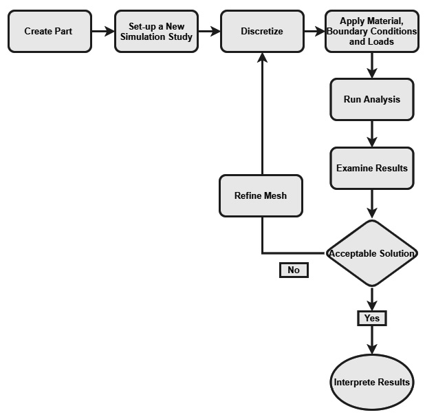
Figure 1.1 – Flowchart for the static analysis of a one-member component
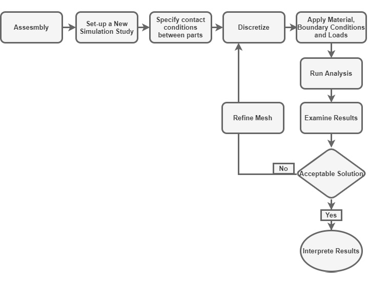
Figure 1.2 – Flowchart for the static analysis of an assembly
A couple of comments regarding the steps indicated in Figure 1.1 and Figure 1.2 are provided as follows:
- The first step to the simulation of a product (such as a part or an assembly) is to create its CAD model. At this stage, all geometric properties are defined. For complicated geometries, the geometry of the structure to be analyzed might have to be defeatured and fine-tuned.
- Next, the SOLIDWORKS Simulation interface is launched.
- Discretization of the part or assembly is carried out. Often, discretization is called meshing. This refers to the crucial process of dividing a part or assembly into smaller pieces (similar to LEGO pieces). A few concepts need to be known regarding meshing:
- Meshing creates elements and nodes.
- An element describes a finite-sized division created from the original component to be analyzed.
- Elements are joined by common points called nodes.
- Each finite element is characterized by a specific number of degrees of freedom. A degree of freedom is the fundamental field variable calculated during the FEA. For instance, for static analysis problems, the displacement vector is the main degree of freedom during the computation. However, in the case of simulations related to thermal analysis problems, the degree of freedom is temperature.
- The size and type of elements created during meshing are key to getting accurate results. Typically, the types of elements to be used for analysis become obvious from the nature of the problem. This concept will be developed further throughout the book.
- After the discretization step, we will specify the following:
- Material properties. For static analysis, this will generally include stiffness information such as Young's modulus and Poisson's ratio.
- Loads. A variety of loads can be applied within the SOLIDWORKS Simulation interface, ranging from axial load, transverse load, torsional load to pressure load.
- Fixtures. In the language of SOLIDWORKS Simulation, the word "fixture" is used to indicate boundary conditions. Meanwhile, boundary conditions generally refer to physical constraints on the movement of specific joints or segments of a load-bearing structure. They arise from the presence of supports used to ensure that a structure being analyzed is properly constrained to prevent rigid body motion during the application of external loads.
- Connections. In the language of SOLIDWORKS Simulation, the connections settings comprise the contact condition that is required anytime two or more components touch each other before or during the simulation process. This might arise from welding, bonding, riveting, or various other types of joining of a practical nature. SOLIDWORKS Simulation provides a variety of contact types that will be explored as we progress in our exploration of the software.
- Finally, we run the analysis, then obtain and interpret the results.
Information
In FEA, elements of different shapes, degrees of freedom (DOF), and complexity exist. In principle, when the term DOF is used in mechanics, it denotes the number of independent quantities required to describe a displaced or perturbed state of a structure. For static problems that are the focus of this book, we will be using DOF to refer to the number of possible displacement components at nodes of a specific finite element. Note that a comprehensive account of the mathematical derivations for a wide variety of elements is not addressed in this book. Such derivations can be found in many of the books on the mathematical foundation of the FEM such as [3] and [4].
Elements within SOLIDWORKS Simulation
SOLIDWORKS Simulation has three major families of elements that are used in the performance analysis of components:
- Continuum elements:
- Solid elements
- Two-dimensional (2D) plane elements
- Structural elements:
- Beam elements
- Truss elements
- Shell elements
- Special elements
While these elements will be rigorously explored in subsequent chapters, Table 1-2 highlights three representative cases of when to use these elements.
Generally, a solid element is used for bulky models with considerable thickness and volume. 2D plane elements are employed for the 2D analysis of members (such as axisymmetric, plane stress, or plane strain problems). Beam and truss elements are used for the analysis of structural members that have one of their dimensions far greater than the dimensions of their cross-sections. Shell elements are deployed for thin-walled members. The special elements mostly connect elements such as springs elastic supports, and more:
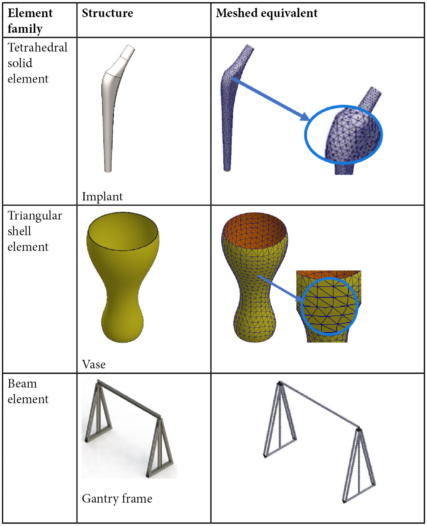
Table 1-2: Discretization and the major types of elements
Types of SOLIDWORKS Simulation license
SOLIDWORKS Corporation offers three types of license for SOLIDWORKS Simulation:
- SOLIDWORKS Simulation Standard
- SOLIDWORKS Simulation Professional
- SOLIDWORKS Simulation Premium
Of these three, the premium license is the most comprehensive in terms of capability. The professional license does not support nonlinear and composite analyses. The standard license is even more limited in terms of the scope of analyses it supports. For this book, the premium license is employed.
Information
To read more about the kinds of analyses that can be carried out with each of the previously mentioned licenses, please visit https://www.solidworks.com/product/solidworks-simulation.
Computing requirements
SOLIDWORKS is a memory-hungry application. This is understandable given the functionalities that are packed into this amazing piece of software. For best performance, the recommendation listed in Table 1-3 is suggested for PCs or laptops to be used for basic analysis with the SOLIDWORKS Simulation:

Table 1-3: System requirements
Information
For further information about system requirements, beyond the details in Table 1-3, head over to https://www.solidworks.com/support/system-requirements.
What are the limitations of SOLIDWORKS Simulation?
While SOLIDWORKS Simulation is a powerful tool that can be used for numerous kinds of analyses of products and components, it is worth mentioning that it has a limited number of elements in its library. This point should be borne in mind while dealing with multiphysics problems for which a suitable element for the analysis might not exist in the SOLIDWORKS Simulation library. Besides, you should always find alternative methods to determine the accuracy of the results retrieved from the SOLIDWORKS Simulation. This is known as validation, and it can be done via experiments or analytical techniques at one stage of the product development phases. The approach to such methods of validation through experimental stress techniques is not covered in this book (a classic reference is a text by Dally and Riley [5]).
This wraps up our presentation of the overview of the SOLIDWORKS Simulation. In the next section, we will do a cursory examination of the SOLIDWORKS interfaces.
Understanding the SOLIDWORKS interfaces
The main focus of this section is to briefly introduce the SOLIDWORKS interfaces. Since we are going to be interacting with the interface in the rest of the book, only a few of the features are examined. Nonetheless, it is worth pointing out that the SOLIDWORKS Simulation interface is closely linked with the SOLIDWORKS modeling environment, and both require that you have the correct license. With SOLIDWORKS installed on your PC or laptop, the interfaces are accessed by following the steps laid out in the subsections that follow.
Getting started with the SOLIDWORKS modeling environment
This subsection illustrates a brief interaction with the SOLIDWORKS 2021-2022 modeling environment. The steps focus on the use of a single-part component to reveal the simulation environment. Let's start by launching the SOLIDWORKS application and then navigating to the modeling environment by following these steps:
- Choose File from the main menu.
- Click on New.
- Select Part and click on OK:
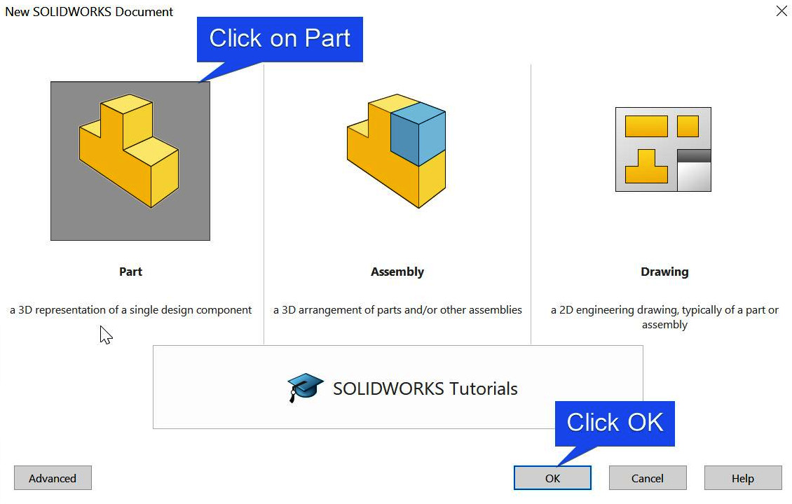
Figure 1.3 – The steps for launching the modeling environment
The modeling environment is launched after completing the preceding steps, as shown next. Generally, the modeling environment features many items, as shown in Figure 1.4. This includes the following:
- Menu Bar: This provides access to different kinds of commands that the software offers.
- Command Manager Tab: This encompasses a series of tabs segregating the commands for many specialized tasks.
- Feature Manager Tree: This acts as a record of features that are created in the graphics window, often representing these features in the order in which they are created.
- Document Window: This is used to navigate between different windows in the graphics area.
- Graphics area: The major area for modeling and simulation activities:

Figure 1.4 – The SOLIDWORKS 2021-2022 user interface
With the basic information about the interface detailed, let's now take a brief look at how to activate the simulation environment. We will come back to this activity in subsequent chapters in more detail.
Activating the SOLIDWORKS Simulation environment
Launch the SOLIDWORKS Simulation interface by following these steps:
- Activate the simulation add-in by performing the following:
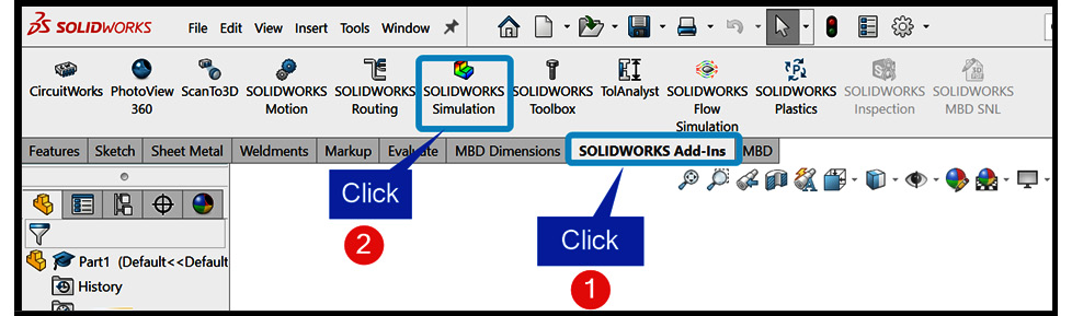
Figure 1.5 – Activating the SOLIDWORKS simulation add-ins
The Simulation tab becomes active, as shown next. However, notice that when the SOLIDWORKS Simulation becomes activated, most of the icons are gray, as shown in Figure 1.6. This arises from the fact that no analysis has been defined yet.
- Start a new analysis by performing the following:

Figure 1.6 – Starting a new simulation study
- Select a Study type (in this book, we will be restricted to static analysis).
- Supply a descriptive name for the simulation study, as shown in Figure 1.7.
- Click on OK:
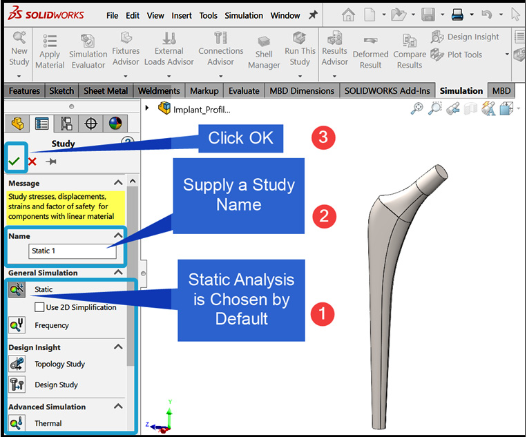
Figure 1.7 – Supplying the details of the simulation study
In response to the preceding steps, the simulation study environment is activated, as indicated in Figure 1.8. There are a few things to pay attention to in this screenshot. For one, the different icons that were previously gray underneath the Simulation tab in Figure 1.6 are now active in Figure 1.8. Further, the simulation tree manager and the study tab (at the base of the screen) have both appeared:
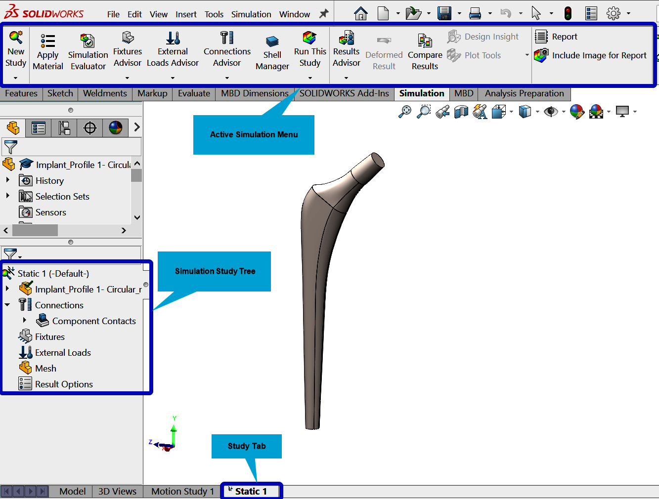
Figure 1.8 – Simulation study tree
The SOLIDWORKS Simulation environment is better explored within the context of simulation problems. Accordingly, rather than detailing all the features here, we will further examine them comprehensively in subsequent chapters and reveal the power of this simulation engine for the analysis of various types of problems.
In the next section, we will briefly highlight some of the important updates in SOLIDWORKS Simulation 2021-2022.
What is new in SOLIDWORKS Simulation 2021-2022?
SOLIDWORKS 2021-2022, upon which this book is based, is the latest version of SOLIDWORKS with significant improvement in functionality and performance. In terms of its look, SOLIDWORKS 2021-2022 appears similar to the previous version of SOLIDWORKS (specifically, the 2020-2021 version). However, there are important differences across many phases of the software. Nonetheless, when it comes to the 2021-2022 version of SOLIDWORKS Simulation, a few of the updates are highlighted here:
- Change in terminology for the items under the Connections folder within the simulation study tree: For instance, if we import the model of an assembly into the modeling environment and then launch a New Study (as done in Figure 1.6), the look of the Simulation study tree in the 2021-2022 and the 2020-2021 versions will be similar to Figure 1.9:
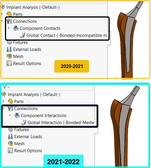
Figure 1.9 – A highlight of the difference in the Simulation study tree
As you can see, Component Contacts is now known as Component Interactions, while Global Contact becomes Global Interaction.
- Update to the Static Options dialog box: After launching a new study environment, you can examine the Static Options dialog box by following Figure 1.10:
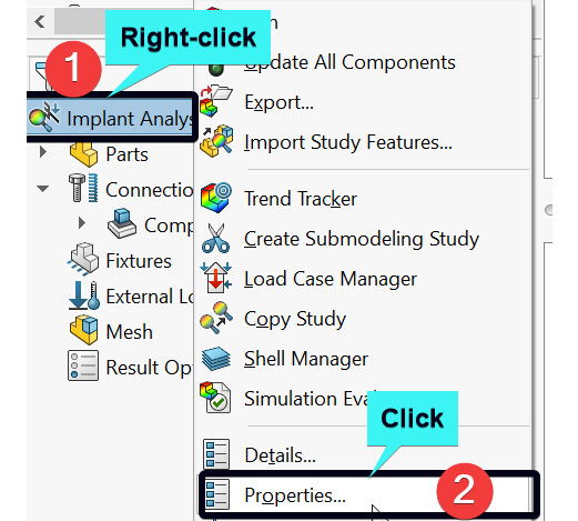
Figure 1.10 – Initiating the static options dialog box
After clicking on Properties…, the Static options dialog box appears. As shown in Figure 1.11, the Static options dialog box for the 2021-2022 version has a more streamlined interface for modifying various study properties.

Figure 1.11 – Partial views of the static options dialog box
Additionally, as you will note from Figure 1.11, in the 2021-2022 version, the Automatic Solver is selected by default within the static options dialogue box. And talking about the static options dialog box, the number of solution Solvers available in the 2021-2022 version is the same as the earlier version, as shown in Figure 1.12. However, the FFEPlus solver, which is based on an iterative technique is now more powerful (this is true for the other solvers as well):
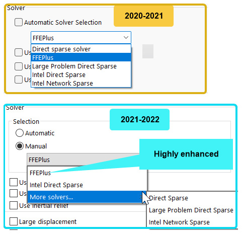
Figure 1.12 – The Solver options within the static options dialog box
Apart from the aforementioned update, we can now shift our attention briefly to the update to the Connections folder's sub-items.
- Update to the Connections folder context menu. It is shown in Figure 1.9 that there is a change in terminology concerning the Connections folder sub-items under the Simulation study tree. The update is deeper than what was highlighted in Figure 1.9. To see another update, you should right-click on the Connections folder. From the right-click context menu, you will notice that the items named Contact Set... and Component Contact... are now referred to as Local Interaction... and Component Interaction... , as depicted in Figure 1.13:
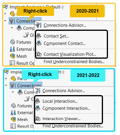
Figure 1.13 – Highlight of the update to the Connections folder context menu
We will expand on this change in more detail in Chapter 6, Analyses of Components with Solid Elements, and Chapter 7, Analyses of Components with Mixed Elements.
- Update to the Mesh PropertyManager: If you right-click on the Mesh folder within the Simulation study tree and then select Create Mesh, you will observe a difference in the arrangement of the meshing engines, as shown in Figure 1.14:
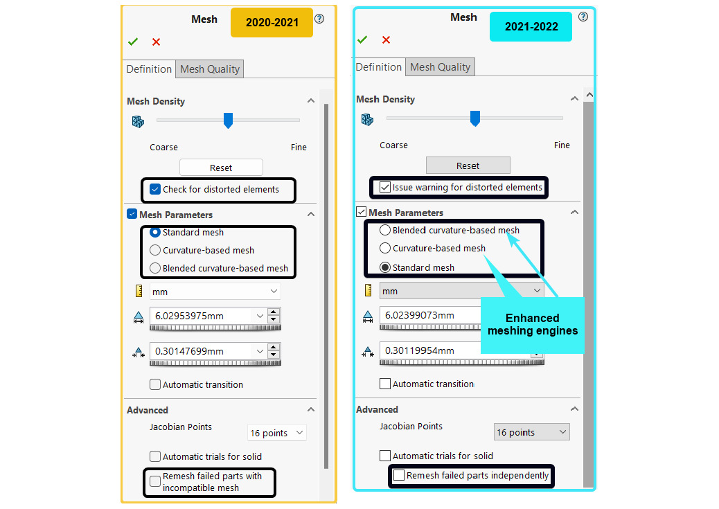
Figure 1.14 – Highlight of the change for the Mesh PropertyManager
While the names of the meshing engines remain the same, as shown in Figure 1.14, the Curvature-based mesh and the Blended curvature-based meshing engines have undergone serious updates to facilitate enhanced accuracy of the simulation results. Again, we will revisit the issues around meshing in the second and third sections of the book.
This ends our discussion of a few of the differences that exist in the 2021-2022 SOLIDWORKS Simulation. So far, we have primarily focused on the updates that will be discussed in the later chapters of the book. For a more detailed look at the significant enhancements across all aspects of SOLIDWORKS, in general, and SOLIDWORKS Simulation, in particular, you should check out https://www.solidworks.com/product/whats-new.
Summary
This chapter provided a short overview of the importance, applications, and basic concepts of finite element simulation (such as discretization, elements, the types of elements, nodes, the main phases in finite element simulation, and more). We also initiated our exploration of the theme of this book by introducing the SOLIDWORKS general interface and the SOLIDWORKS Simulation interface.
Subsequent chapters of the book will take a detailed look at the use of SOLIDWORKS Simulation for the analyses of different kinds of structures. In the next chapter, we will examine the analysis of bars and trusses.
Further reading
- [1] The finite element in plan stress analysis, in Proceedings of the 2nd ASCE Conference on Electronic Computation, R. W. Clough, Pittsburgh, PA, 1960,
- [2] The finite element method in structural and continuum mechanics: numerical solution of problems in structural and continuum mechanics, O. C. Zienkiewicz and Y. K. Cheung, London; New York: McGraw-Hill (in English), 1967.
- [3] Introduction to the Finite Element Method, J. N. Reddy, McGraw-Hill Education, 2019.
- [4] Fundamentals of Finite Element Analysis, D. V. Hutton, McGraw-Hill, 2003.
- [5] Experimental Stress Analysis, J. W. Dally and W. F. Riley, McGraw-Hill, 1978.