Chapter 7: Analyses of Components with Mixed Elements

Thus far in this book, we have explored simulation examples in which components are discretized using a single family of elements. However, as can often happen with many complex practical design problems with diverse functional components, you will face situations where the goal will be to put these elements together in one single simulation task. Consider, say, the simulation of car frames, building frameworks, or plane fuselages with all the flooring details and connections. By taking advantage of putting different elements together, you can accelerate the simulation runtime or reduce the computational resources required to achieve your simulation objectives.

For the above reason, the elements you have seen in the previous chapters will make a re-appearance again in this chapter. We will examine two case studies, and our discussion will orient around the following topics:

• Analysis of three-dimensional components with mixed beam and shell elements
• Analysis of three-dimensional components with mixed shell and solid elements

Technical requirements

You will need to have access to the SOLIDWORKS software with a SOLIDWORKS Simulation license.

You can find the sample files of the models required for this chapter here: https://github.com/PacktPublishing/Practical-Finite-Element-Simulations-with-SOLIDWORKS-2022/tree/main/Chapter07.

Analysis of three-dimensional components with mixed beam and shell elements

This section details our first case study, which centers around an analysis that involves a mixture of beam elements and shell elements.

As you will recall, we pointed out the attributes of the beam element in Chapter 3, Analyses of Beams and Frames, while those of the shell elements were described in Chapter 5, Analyses of Axisymmetric Bodies. Although their dimensionality is different (one being a line-based element and the other being a triangular element), both of these elements as implemented in SOLIDWORKS Simulation have six degrees of freedom (DOFs) per node. Notably, these DOFs are the three translational displacements along the X, Y, and Z axes, and the three rotational displacements about these three axes. Putting these two elements together in the first case study, therefore, represents a good starting point in the exploration of analyses with mixed elements. Overall, the compatibility of the DOFs is one of the more important criteria to consider when employing mixed elements to speed up your simulation. If you want to dig deeper into other practical considerations for the use of mixed meshing, you may refer to [1].

The premise for the case study is given next.

Problem statement – case study 1

Figure 7.1a shows an idealized assembly representing the basic structural elements of a two-story residential building [2] (see the Further reading section). The major dimensions of the building (height x width x length) are given by 6 m x 6 m x 18 m. The beams and columns supporting the building floors are made of W410x16 ASTM A36 structural steel. Each has the cross-section shown in Figure 7.1b. In addition, the 130 mm thick floor slabs are made of concrete (E = 30 GPa, G = 12.71 GPa, Poisson's ratio = 0.18, ultimate compressive strength = 41 MPa, ultimate tensile strength = 5 MPa, and density = 2300 kg/m3).

We aim to conduct a simplified static analysis of the building under a dead load arising from the self-weights of the structural members and a live load of 2500 N/m2 on the floor slabs. Let's assume the value of the dead load complies with the local residential structural design guide [3]. From the analysis, we shall examine the maximum vertical displacement of the building under these loads and the bending stresses in the beams and the columns.

Figure 7.1 – The model of a partitioned two-story building

In what follows, we will address the problem in four major sections designated as Part A: Reviewing the structural models, Part B: Creating the simulation study, Part C: Meshing and running, and Part D: Post-processing of results.

Let's begin.

Part A: Reviewing the structural models

To get you started, the files of the models we need have been provided. This means you should download the Chapter 7 folder from the book's website to retrieve the models. Inside the folder, you will see the following items:

• A SOLIDWORKS part file named Two-story
• A SOLIDWORKS part file named Two-story-Solar
• A folder named Custom

On the one hand, the first and second items pertain to the full model of the two-story buildings for case studies 1 and 2, respectively. On the other hand, the third item is a folder that contains the file of the sketched profile shown in Figure 7.1b.

We will briefly go over the first and third items in the next sub-sections. The second item will be briefed when we get to our second hands-on.

Copying and reviewing the file in the custom profile

First, let's clarify why we need the Custom folder. You will recall that we introduced the weldment tool in Chapter 2, Analyses of Bars and Trusses, and it was also employed in Chapter 3, Analyses of Beams and Frames. In those chapters, we worked with the original weldment profiles from the SOLIDWORKS library. On the contrary, the cross-section shown in Figure 7.1b is not available in the SOLIDWORKS weldment database. The consequence of this is that we need to create this new profile. Once the profile is created, it should be saved in a separate folder to distinguish it from the SOLIDWORKS original files. This is the reason for having the Custom folder for this chapter.

Meanwhile, for SOLIDWORKS to have access to the profile we created, the Custom folder has to be placed in the SOLIDWORKS weldment profiles directory. To accomplish this, follow these steps to move the Custom folder to the SOLIDWORKS weldment profiles directory:

1. Navigate to the Chapter 7 folder that you have downloaded.
2. Copy the folder named Custom (using the normal Windows file copying procedure).
3. Paste the folder into the SOLIDWORKS in-built weldment directory at the following address: Drive:Program FilesSOLIDWORKS CorpSOLIDWORKSlangenglishweldment profiles).

   After pasting, you should see the Custom folder among the other directories as shown in Figure 7.2.

Figure 7.2 – The default and the custom directories

You should examine the content of the Custom folder to see that it has another sub-folder called Custom_ISO. In turn, this sub-folder contains the created profile (W410 x 60) as depicted in Figure 7.3.

Figure 7.3 – Custom folder for the created profile

You will require administrator rights on the computer you are using to be able to copy into the SOLIDWORKS in-built weldment directory.

Note on Weldment

We explored the default weldment profile in Chapter 2, Analyses of Bars and Trusses, in the sub-section, Introducing the weldments tool. Further, in that chapter, we examined the content of the ansi inch and iso folders shown in Figure 7.2. More importantly, for a brief description of how to create a custom profile such as W410 x 60, a pertinent resource is the official SOLIDWORKS help link: https://help.solidworks.com/2021/English/SolidWorks/sldworks/t_Weldments_Creating_a_Custom_Profile.htm.

Note that steps 1–3 implicitly assume that you have never created a custom weldment sub-directory before. However, if you already have a specific folder for your custom weldment profiles, you should only copy and paste the W410 x 60.SLDLFP file into that folder.

With the custom profile copied into the SOLIDWORKS library, we shall now take a look at the file of the building (that is, Two-story).

Reviewing the file of the building

To go over some of the features of the model of the building, follow these steps to bring the file up for examination:

1. Start up SOLIDWORKS.
2. Select File  Open, then open the part file named Two-story (which you downloaded).
3. Navigate to the Feature Manager design tree and examine the details as shown in Figure 7.4.

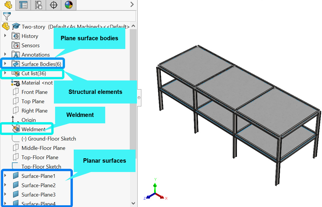
Figure 7.4 – Review of components

Figure 7.4 points to the fact that we have 6 surface bodies to idealize the concrete slabs and 36 cut lists to represent the structural elements (beams and columns). Further, you can see that we have used the planar surface tool (Insert  Surface  Planar) to create the surface bodies, while the structural elements have been created using the weldment tool.

With the files reviewed, we are now primed to tackle the simulation tasks.

Part B: Creating the simulation study

This section details some of the necessary preprocessing routines (the activation of the simulation study, assigning of material, application of fixtures, and specification of loads).

We begin with the activation of the simulation environment.

Activating the Simulation tab and creating a new study

To activate the simulation commands, we follow the steps highlighted next:

1. Under the Command manager tab, click on SOLIDWORKS Add-Ins, then click on SOLIDWORKS Simulation to activate the Simulation tab.
2. With the Simulation tab active, create a new study by clicking on New Study.
3. Input a study name within the Name box, for example, Two-story analysis.
4. Keep the Static analysis option.
5. Click OK.

In response to the completion of steps 1–5, the model is transformed in the simulation environment with the joints created at the connection points of the beams and the columns as shown in Figure 7.5a.

Figure 7.5 – Simulation property manager

Looking at the simulation study tree (partially depicted in Figure 7.5b), you will notice the 6 surface bodies and the Cut-List folders comprising the beams and columns. Coupled with the previous detail, you will observe that the thickness has not been defined for the surface bodies as highlighted in Figure 7.5b. So, our next focus is to define the thickness.

Assigning thickness

The surface bodies will be discretized using shell elements during the meshing process. For this reason, we need to define the thickness using the Shell Definition tool. Follow these steps to assign thickness:

1. Within the simulation study tree, select all 6 surface bodies, right-click within the selected area, then select Edit Definition... as shown in Figure 7.6.
   

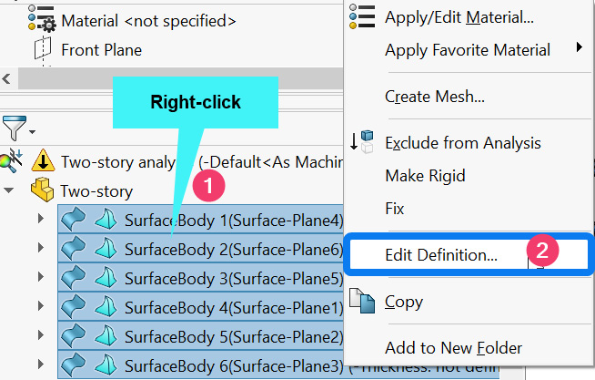
   Figure 7.6 – Initiating the thickness definition for the surface bodies

   Within the Shell Definition property manager that appears, perform the following actions.

2. Under the Type option, select Thin as shown in Figure 7.7.
   

   Figure 7.7 – Shell Definition property manager

3. Within the thickness value box (labeled 2 in Figure 7.7), key in 130 mm.
4. Check the box labeled 3 (Flip shell top and bottom).
5. Activate the Full preview option.
6. Under Offset, ensure the mid-surface option is selected.
7. Click OK.

This completes the specification of both the thickness of the surface bodies and the choice of a thin shell assumption. A quick remark on step 4. Essentially, we have used this step to distinguish which face of the shell elements the pressure load acts upon. This step is crucial anytime we create a surface body using the planar surface tool. The application of external loads or supports on the wrong side of shell elements may at times throw some unexpected behavior.

Further Comments on Shell Faces

When we employed shell elements in Chapter 5, Analyses of Axisymmetric Bodies, (in the sub-section Assigning thickness) we did not have to flip the face of the shell during the shell definition. You may be wondering why. Mainly because we created the surface from the inner face of the revolved body (you may refer to Figure 5.12). SOLIDWORKS will treat the face from which the thickness is created as the positive face, and hence the face to which loads, boundary conditions, and so on, should be applied. In the current case, what we have is just a plane surface with no pre-defined positive or negative faces, so we need to manually ensure the right face is referenced as the top or bottom.

It is now time to assign materials to the structure.

Creating and assigning a custom concrete material property

We shall start by assigning the material property to the floor slabs (made of concrete according to the problem statement). Regrettably, the SOLIDWORKS library does not contain a concrete material, which means we need to create it.

To this end, let's create and apply the concrete material properties as outlined next:

1. Within the simulation study tree, select all six surface bodies and right-click within the selected area of the selected items.
2. Click Apply/Edit Material....

   From the materials database that appears, take the next set of actions.

3. Scroll down to the material folder named Custom Materials, right-click, then click New Category (Figure 7.8a). In response to this, a new material folder will be created with the default name being New Category.
4. Change the name to MyConcrete (Figure 7.8b).
   

   Figure 7.8 – Navigating to the custom material section

5. Next, right-click on the newly created MyConcrete folder and select New Material from the context menu that appears (Figure 7.9a). With this step, a new material file will be created with the default name Default. Change the name to Concrete as shown in Figure 7.9b.
   

   Figure 7.9 – Actions to create a custom concrete material

   At this juncture, we have created the folder and the file for the concrete material. We are now ready to supply all the necessary values.

6. Within the Material database window, for Model Type, select Linear Elastic Isotopic and ensure the unit remains as SI - N/m^2 (Pa) (labeled 2 in Figure 7.10).
7. For the failure criterion, select Mohr-Coulomb Stress (labeled 3 in Figure 7.10).
8. For the material property values, follow the details in the box labeled 4 in Figure 7.10.
9. Click Save, Apply, and Close (in that order).
   

Figure 7.10 – The material database with the details of the custom concrete

It is important to point out we have selected the Mohr-Coulomb Stress failure theory in step 7 to be consistent with a simplified status of concrete as a brittle material [4].

A Note on Failure Criteria

You can also read about the various failure criteria in SOLIDWORKS Simulation on the help page: https://help.solidworks.com/2022/english/SolidWorks/cworks/Failure_Criteria.htm?verRedirect=1.

With steps 1–9 completed, we are done with the creation and application of the concrete material properties. As usual, a check mark should appear on the six surface bodies in the simulation study tree.

Next, we shift to the application of the material property to the beams and the columns.

Assigning material details to the beams/columns

Since the ASTM A36 material comes with SOLIDWORKS, the procedure here is straightforward. The steps to assign the ASTM A36 material property to the beams and columns are as outlined:

1. Right-click on the Cut-List folder and choose Apply/Edit Material… (Figure 7.11).
   

   Figure 7.11 – Assigning a material to the bodies

2. From the materials database that appears, expand the Steel folder, then click on ASTM A36 steel.
3. Click Apply and Close.

The material assignment task is now completed. In the next sub-section, we will briefly take a look at the contact setting (before we deal with the application of the load and the specification of the fixture).

Examining the default contact setting

Due to the presence of multiple interacting parts, interaction conditions must be defined between them. By expanding the Connections folder as shown in Figure 7.12, you will notice that SOLIDWORKS has applied a global interaction (Bonded) at the assembly level for us.

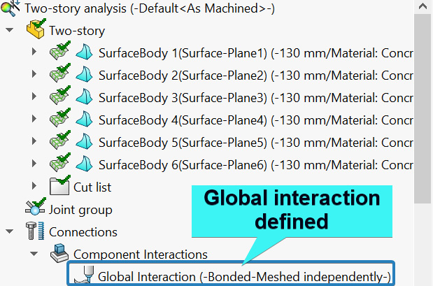
Figure 7.12 – Examining the interaction details

For this case study, the Bonded option is sufficient to hold all the parts together as a single piece, and there's no need to override it (later on in case study 2, we will need to go beyond the default contact). With this, we are done with the examination of the contact setting, and we can now transition to the application of the fixture.

Applying fixtures at the base of the lower columns

For the boundary conditions, otherwise known as fixtures within the SOLIDWORKS Simulation environment, we shall constrain the base of the building. To achieve this, follow the next set of steps:

1. Right-click on Fixtures and pick Fixed Geometry from the context menu that appears.
2. When the Fixture property manager appears, click on the Joints symbol (labeled 2 in Figure 7.13).
3. Navigate to the graphics window and click on the six bottom joints as shown in Figure 7.13.
4. Click OK.

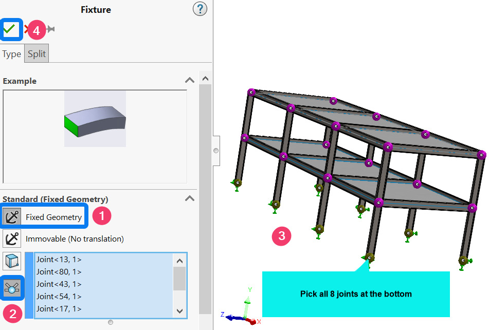
Figure 7.13 – Defining the fixed boundary supports at the base

With the completion of the application of the fixed boundary condition, let's now move on to the application of the loads.

Applying external loads

We have two loads to be applied to the building – the pressure and the gravitational loads. To apply these, follow the steps outlined next:

1. For the pressure load, right-click on External Loads, select Pressure, then follow the options indicated in Figure 7.14, and click OK to wrap up the selections.
   

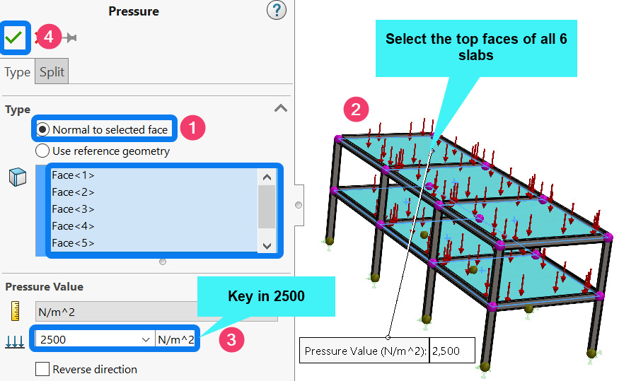
   Figure 7.14 – Options for the application of the pressure load

2. For the gravitational load, right-click on External Loads and select Gravity (Figure 7.15).
   

   Figure 7.15 – Initiating the application of the gravity load

   Within the Gravity property manager that appears, execute the following actions.

3. Click inside the plane reference box (labeled 1 in Figure 7.16) and navigate to the graphics window to select Top-Floor Plane.
4. Check the Reverse direction box (labeled 3 in Figure 7.16), then click OK to wrap up the selections for the gravity load.

Figure 7.16 – Application of the gravity load

Over the past sub-sections, we have ticked a few items off the list of the preprocessing tasks. Specifically, we have seen how to define thickness for a surface created using a planar surface and how to flip its faces to have the right area for load application. We assigned material properties, which included steps to create a custom concrete material. Moreover, we've reviewed the contact settings, applied the fixture, and demonstrated the application of gravity and pressure loads. In the next sub-section, we shall transition to the meshing and post-processing phases of the workflow.

Part C: Meshing and running

In previous chapters, we have seen and discussed various ways to create a mesh. For this case study, the model involves mixed bodies (weldments for the beams and columns and surface bodies for the concrete slabs). Consequently, the meshing engine will discretize the beams/columns using beam elements, while the slabs will be discretized using shell elements as will be demonstrated in the sub-section that follows.

It is possible to create a mesh without giving thought to how it is done by simply using the Create Mesh command. But due to the fact that we have mixed elements for this case study, the approach we will adopt is to create mesh controls for the beam elements and use the default mesh setting for the shell elements.

To create the mesh controls and the mesh, take the following steps:

1. Right-click on Mesh and select Apply Mesh Control.
2. From the Mesh Control property manager that pops up, under Selected Entities, activate the beam option (labeled 1), then follow the other illustrations in Figure 7.17, and wrap up the selections by clicking OK. You are encouraged to use the box selection approach when selecting the beams.
   

   Figure 7.17 – Mesh control options for the beams

   The box labeled 3 in Figure 7.17 implies that we shall be discretizing all beams and columns with 15 elements each. Next, we generate the mesh for the whole assembly.

3. Right-click again on Mesh, then select Create Mesh. When the Mesh Control property manager appears, keep the options as shown in Figure 7.18, and wrap up the selections by clicking OK.
   

   Figure 7.18 – General meshing options

4. After the running is complete, you can view the mesh by right-clicking on Mesh and then selecting Show Mesh. The top view of the meshed structure is shown in Figure 7.19a.
   

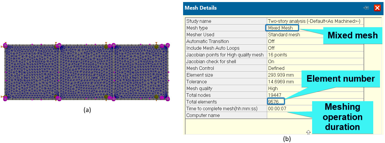
   Figure 7.19 – (a) Top view of the meshed structure; (b) mesh details

5. Before we process the results, you can view the mesh details by right-clicking on Mesh and then selecting Details. The meshed detail is shown in Figure 7.19b.
6. To obtain the results, right-click on the analysis name and select Run. It will take some time to finish running.

Looking at the mesh details in Figure 7.19b, we can infer that: (i) the mesh quality is moderate; (ii) we have a mixed mesh with a total of 9,576 elements created via the Standard Meshing engine; and (iii) and the duration of the meshing run is minuscule.

With the activities about the meshing out of the way, let's now examine the results.

Part D: Post-processing of results

We aim to address the following questions:

• What is the maximum vertical deflection of the structure?
• What is the nature of the bending stresses in the beams/columns?

Let's kick off with the first question.

Obtaining the displacement result

To obtain the vertical displacement, we follow these steps:

1. Right-click on Results, then select Define Displacement Plot.
2. Within the Displacement plot property manager that pops up, under the Definition tab, navigate to Display and select UY: Y Displacement as highlighted in Figure 7.20a.
3. Also, move to the Chart Options tab and make the selections indicated in Figure 7.20b.
4. Click OK to finish off the selections.

Figure 7.20 – Specifying options for the displacement plot

Figure 7.21 depicts the vertical deformation (which is the displacement along the Y-axis) of the whole structure.

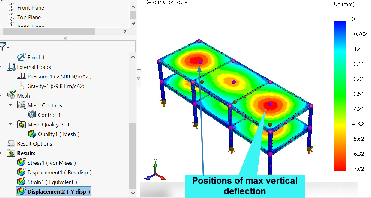
Figure 7.21 – The plot of the vertical deflection of the structure

It can be seen from Figure 7.21 that a maximum vertical deflection of -7.02 mm is obtained as a consequence of the combined effect of a live load of 2,500 N/m2 acting on the slabs and the self-weights of the whole structure. Besides that, the figure also signals that the location of the maximum deflection is at the center of the right and left upper slabs.

As much as we would like to move on to the next result, it is important to ask: How reliable is the value of displacement we have obtained? Before answering this question, recall that it has been pointed out in the past chapters that a simulation study should ideally be verified and validated before deriving technical conclusions from it. The validation could be through theoretical calculation, experiments, or data from other reliable sources.

Interestingly, unlike the past chapters, the complexity of the analyzed structure makes it difficult to have a closed-form solution via a theoretical framework to validate the value we have obtained. This kind of situation is prevalent in so many practical situations. And under such circumstances, an experiment may have to be conducted on a scaled-down version of the model to ascertain the accuracy of the simulation results. However, in the present case, in place of conducting an experiment, a similar analysis was carried out in Ansys (another simulation software). Figure 7.22 depicts the displacement plot/result from Ansys.

Figure 7.22 – Vertical deflection of the structure from Ansys

As you can see, the maximum displacement results from SOLIDWORKS Simulation (in Figure 7.21) and the results from Ansys (in Figure 7.22) only differ by around 2.4% despite using a moderately defined mesh. Just to be clear, it is not a normal practice to have to do this comparison with other software (especially in companies with limited resources). We have done this comparison just to reinforce our confidence in the reliability of the SOLIDWORKS Simulation result.

Meanwhile, we have focused on the vertical deflection here because the two loads are directed along the Y-axis. In a more elaborate analysis, it may be desirable to include the effect of wind load in a specific direction, say along the Z-axis. For such a scenario, it is best to look at the resultant displacement of the whole building. Besides, if a seismic analysis is the purpose of the simulation, then a quasi-static or dynamic analysis may have to be conducted.

Relatedly, we may also uncover further details about the structure from the stresses that develop within the members. For this reason, we will now proceed to examine the stress results in the next sub-section.

Extracting the stresses in the components

We shall restrict ourselves to the bending stresses in the beams/columns. In this vein, follow the steps given next to obtain the bending stresses:

1. Right-click on the Results folder, then select Define Stress plot.
2. Within the Stress plot property manager that appears, under Display, activate the Beams option, then follow the selections shown in Figure 7.23.
   

   Figure 7.23 – Specifying options for the bending stress along direction 1

3. Now, move to the Chart Options tab. Under Position/Format, change the number format to floating.
4. Click OK.

With steps 1–4 completed, the graphics window is updated with the plot of the bending stress along direction 1 (X-axis) as depicted in Figure 7.24. As you will notice from the stress plot, the compressive and tensile bending stresses in the members are roughly -38 MPa/+38 MPa. These values are far below the yield strength of ASTM 36 steel, from which the members are made, and will consequently yield acceptable von Mises stress.

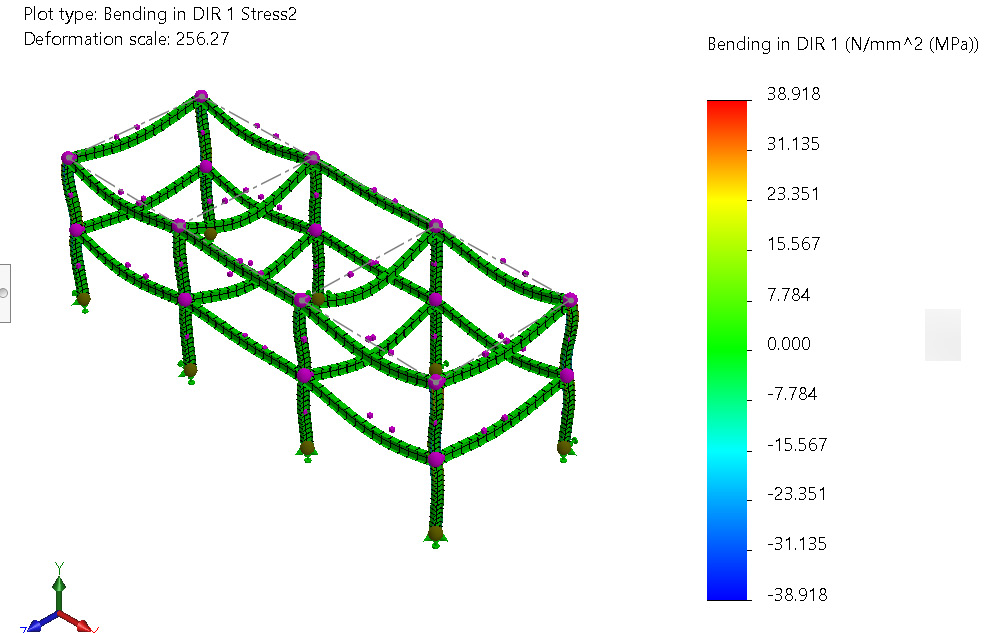
Figure 7.24 – The deformed shape of the beams for the bending stress along the X-axis

Moreover, Figure 7.24 signifies that the exterior columns are the most affected by the bending stress along the X-axis.

Next, if you repeat steps 1–4 to obtain the stress along direction 2 by choosing Bending in DIR 2 (see Figure 7.23), the result should be similar to Figure 7.25.

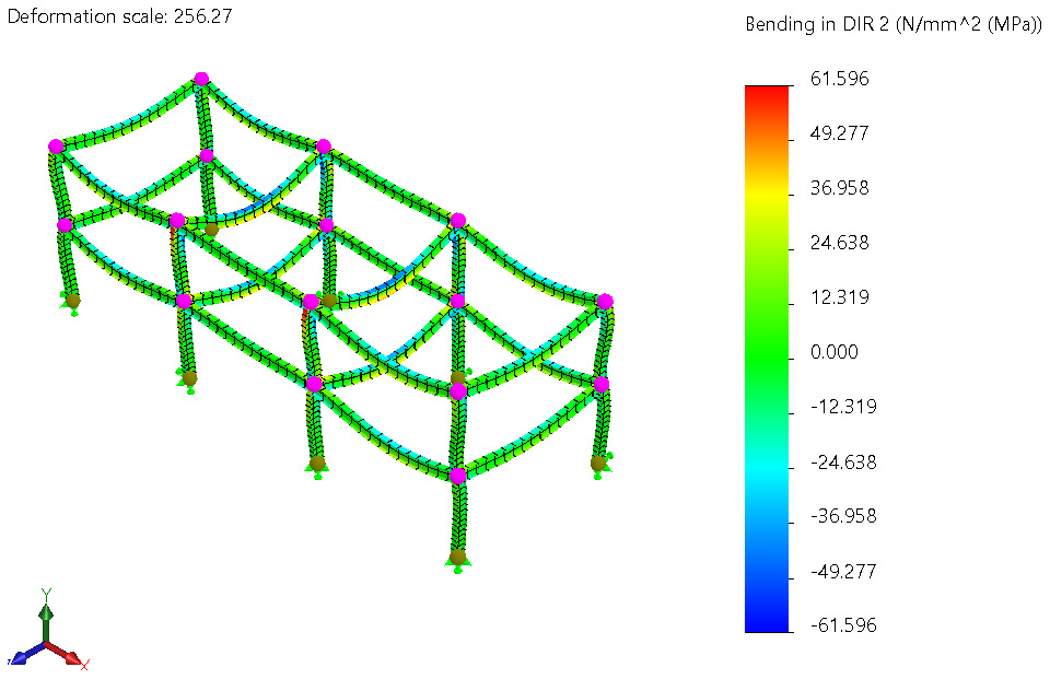
Figure 7.25 – The deformed shape of the beams for the bending stress along the Z-axis

Figure 7.25 reveals that when the stress is examined along direction 2 (the Z-axis), the interior beams of the upper floor are the most stressed. Besides, the maximum compressive and tensile bending stresses in the members are roughly -61 MPa/+61 MPa. Likewise, these values are not too high to cause concern. Now, although not covered, it is recommended that you scrutinize the stresses in the slabs as well. To sum up, note that the deformed configurations that are shown in Figure 7.24 and Figure 7.25 are just for illustrative purposes; they do not represent the true scale of the deformed configurations of the structure. All in all, the results we have discussed show that the response of the building is within acceptable design criteria. Now, assuming the structural deformation of the building is unsatisfactory, can you suggest ways to improve the design?

We have now completed the simulation and obtained the answers to the questions posed for the case study. In all, the procedure for the solution to the hands-on exploration has been a mix of things we have seen in the previous chapters, such as how to deal with material property assignment and examination of contact settings, and so on. But we also managed to demonstrate a few new things such as (i) the creation of a custom concrete material from scratch; (ii) the initiation of mesh control for each family of mesh types in a mixed element simulation task; and (iii) the combination of a gravitational load with the more traditional load type.

In the next case study, we will extend this problem further. In doing so, you will see how to stabilize a structure using SOLIDWORKS soft springs and how to create a no-penetration interaction between a family of solid elements and shell elements, among other things.

Analysis of three-dimensional components with mixed shell and solid elements

Here is the backstory for our second case study. As part of the drive toward decarbonization, the development of solar roof collectors has emerged as one of the simple measures toward the management of the energy crisis confronting our world. This is evident in some of the recent research studies, see for instance [5, 6]. In many cases, these roof-based solar modules are external add-ons to the buildings. This means the effect they have on the structural response of the building may not have been considered at the initial design stage. This case study, therefore, springs from an attempt to examine this effect.

Problem statement – case study 2

In the next few pages, we wish to extend the previous case study to account for the presence of three 3 m by 3 m solar collectors on the top slabs as illustrated in Figure 7.26. Primarily, our objective is to evaluate the ensuing change in deformation and stress on the beams/columns due to the addition of the solar modules to the roof if they collectively impose a pressure load of 600 N/m2.

Figure 7.26 – The model of the two-story building with three solar collectors

Take note that in what follows, we will not include the nitty-gritty detail of the solar collectors. As a form of simplification, we will only consider the aluminum support structures upon which the pressure load from the solar collectors will be applied. Furthermore, we shall build on the foundations we have established so far to present a condensed exploration of the solution.

In all, this case study assumes that you have completed case study 1. This means the following:

• You have downloaded the Chapter 7 folder from the book website to retrieve the models.
• You have copied the Custom folder into the SOLIDWORKS parent directory for weldment profiles as described in the sub-section Copying and reviewing the file in the custom profile (for case study 1).
• You created the custom concrete materials as explained in the sub-section Creating and assigning a custom concrete material property.

If the preceding tasks have been completed, then we can begin with a review of the new model in the next sub-section.

Reviewing the model and activating the simulation study

Follow these steps to bring up the new model of the building with the integrated solar modules' support:

1. Start up SOLIDWORKS.
2. Select File  Open, then open the part file named Two-story-Solar (from the Chapter 7 folder you downloaded).
3. Navigate to the feature manager tree and examine the details as shown in Figure 7.27.

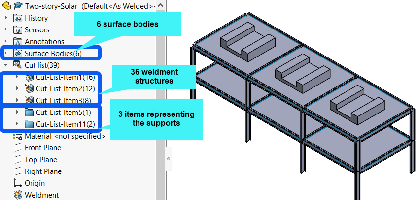
Figure 7.27 – Components of the building with the solar modules' support structures

Figure 7.27 shows that we now have an additional 39 items in the Cut-List folders. This is the sum of 36 structural beams/columns and the 3 new solar supports.

Apart from this, by hiding the three solar module supports, you will observe (as shown in Figure 7.28) that we have introduced the bearing area on the concrete slabs via the Split line tool. The essence of this is to allow us to apply the right component-level contact condition between the solar modules' support structures and the concrete slabs later on during the analysis. Recall that the Split line tool was introduced in Chapter 6, Analyses of Components with Solid Elements.

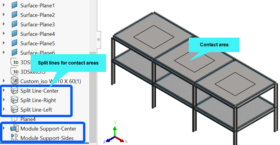
Figure 7.28 – Illustration of contact areas created with split lines

With the basics of the model established, let's now venture into the analysis environment by activating the simulation study as follows:

1. Click on SOLIDWORKS Add-Ins, then click on SOLIDWORKS Simulation to activate the Simulation tab.
2. With the Simulation tab active, create a new study with the name Two-story-Solar analysis (for a guide, see the sub-section Activating the Simulation tab and creating a new study).

Once the simulation study is launched, the simulation study tree should appear as shown in Figure 7.29.

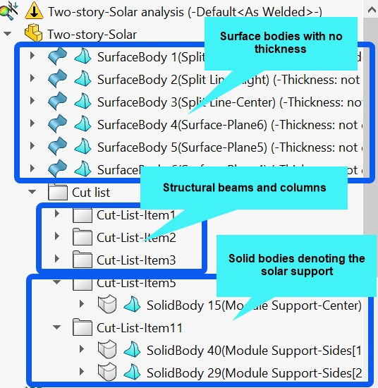
Figure 7.29 – Simulation property manager (building with solar module supports)

It might have caught your attention in Figure 7.29 that when we mesh the structures, we will have shell elements (from the surface bodies), solid elements (from the solar supports), and beam elements (from the structural columns/beams). Additionally, as was the situation in case study 1, the surface bodies have no thickness yet. So, let's address the definition of the thickness and the material properties.

Defining surface thickness and assigning material properties

To assign thickness, the steps are akin to what we described earlier. For this reason, follow the procedure outlined in the sub-section Assigning thickness for case study 1 to assign thickness to the 6 surface bodies.

As for the specification of material properties, we have the surface bodies (made of concrete), the beams/columns (made of ASTM 36 steel), and solar module supports (derived from Aluminium alloy 1060). The steps to specify each of these are highlighted next.

For the surface bodies, do the following:

1. Select all six surface bodies and right-click within the selected area of the selected items as shown in Figure 7.30, then click Apply/Edit Material....
   

   Figure 7.30 – Selecting the surface body for the material properties specification

2. From the material database that appears, navigate to the Custom Materials folder, click on Concrete, click Apply, then click on Close as presented in Figure 7.31.

Figure 7.31 – Assigning concrete to surface bodies

With this, the concrete material properties are assigned to the surface bodies. Next, we resolve the remaining two materials as follows.

For the beams and columns, do the following:

Specify ASTM 36 steel by following the steps described in the sub-section Assigning material details to the beams/columns for case study 1. Note that under the current case, you need to apply material properties one by one on each of the three Cut-List folders for the beams/columns.

For the solar modules' supports, do the following:

1. Within the simulation study tree, select the three solid bodies that represent solar supports as shown in Figure 7.32, right-click within the selected area of the selected items, then click Apply/Edit Material....
   

   Figure 7.32 – Selecting the surface body for the material properties specification

2. From the materials database that appears, expand the Aluminium Alloys folder, then click 1060 Alloy.
3. Click Apply and Close.

This wraps up the specification of the three material properties. Our next focus centers around contact settings.

Updating the default contact/interaction setting

The choice of the interaction setting will either make or break the current case study. Why? You will recall that for case study 1, we revealed that SOLIDWORKS has applied a global interaction setting – Global Interaction (Bonded-Meshed independently-) – at the assembly level for us (see the sub-section Examining the default contact setting). However, for the current case study, this global interaction is not enough because the solar module support structures are not connected to the concrete surface in the sense of "bonding." As a result, we will need to take things a bit further by defining a component-level interaction between the solar modules' support structures and the faces of the concrete slabs.

To enforce the new interaction settings, follow the steps highlighted next (carefully):

1. Within the simulation study tree, expand the Connections folder, right-click on Component Interactions, then select Local Interaction as depicted in Figure 7.33.
   

   Figure 7.33 – Activating the local interactions

   Within the Local Interactions… property manager that appears, we need to execute the next actions.

2. Under Interaction, select Automatically find local interactions.
3. Under Options, select Find shell edge - solid/shell face pairs, then navigate to the graphics window to select the three supports and the top surfaces one by one as shown in Figure 7.34.
   

   Figure 7.34 – Selecting the support structures for the local interactions

4. Still under Options, with the six items (three solid bodies and three surfaces) selected, change back to Find faces (Figure 7.35).
5. Key in a value of 2 mm in the Maximum Clearance box as portrayed in Figure 7.35.
6. Now click the Find local interactions button (see Figure 7.35).
   

   Figure 7.35 – Detecting the local interactions condition

   The three local interactions between the supports and the slabs will appear in the Results box (labeled 1 in Figure 7.36). Scroll down to complete the rest of the actions.

7. Using the Ctrl key, select all three interactions within the Results box (labeled 1 in Figure 7.36).
8. Below the Results box, for Type, ensure the option is set to Contact (labeled 2 in Figure 7.36).
   

   Figure 7.36 – Finalizing the local interactions condition

9. Under Advanced, ensure the option is set to Surface to surface (labeled 3).
10. Click on the green add button beside the Results box (labeled 4).
11. Click OK.
12. After clicking OK, you may get a warning that says Do you want to create the selected local interactions?. Click Yes.

    With steps 1–12 completed, the Connections folder will update to show the new interactions as manifested in Figure 7.37.

Figure 7.37 – The new component interaction sets

Although we briefly highlighted the importance of interactions in Chapter 6, Analyses of Components with Solid Elements, we did not give much detail about them. So, let's step back a bit to look at the interaction definitions for this case study. First, as you can see from Figure 7.37, we now have two different interaction conditions under the Connections folder. Let's highlight the difference between the two:

• Component Interactions: Technically, a component interaction setting defines the contact condition between selected components. Under the component interaction property manager, you may choose to define a global interaction setting for all components in a multi-body component/assembly or a narrower interaction condition between specific components. Indeed, we have adopted Global Interactions (Bonded) in the current study. This holds all the bodies or components together as one piece and it is the default interaction/contact condition for multi-body parts. In situations where this default interaction condition may not be enough, you must define local interactions between selected components.
• Local Interactions: As you can see, in this case study, we have manually defined Local Interactions between specific geometric entities, specifically the faces of bodies that are interacting. It is pertinent to know that a local interaction can be specifically chosen to be any of these: Contact, Bonded, Shrink fit, Free, and Virtual Wall. Obviously, we have used the Contact option here. The Contact interaction generally averts interference between two sets of entities. This means the entities cannot penetrate each other if an external force brings them together, but they can move away from each other. You can explore more information about these options at the following SOLIDWORKS help link: https://help.solidworks.com/2022/english/SolidWorks/cworks/IDH_HELP_FIND_CONTACT_SETS.htm?verRedirect=1.

One more thing before we move on. You will notice that in Figure 7.35, a value of 2 mm was specified inside the Maximum Clearance box. This value can be changed depending on the estimated gap between the surfaces. For the current scenario, a gap of 0.2 mm was maintained between the bearing area of each concrete slab and the face of the solar module's support during modeling. Since this gap falls below the stated maximum clearance value, SOLIDWORKS can automatically determine the contact pairs for the interacting faces.

Important Note

If you are using an earlier version of the SOLIDWORKS Simulation, take note of the following changes in terminology:

Component Interactions in the 2021-2022 version of SOLIDWORKS used to be called Component Contacts in the earlier versions of SOLIDWORKS. Also, Local Interactions in the 2021-2022 version of SOLIDWORKS used to be referred to as Contact Sets in the earlier versions. Moreover, under the Contact Sets property manager (in the earlier versions of SOLIDWORKS), the type of contacts you will see are Bonded, Shrink fit, Allow Penetration, No Penetration, and Virtual Wall. In contrast, in the 2021-2022 version, these options are now known as Contact, Bonded, Shrink fit, Free, and Virtual Wall, respectively.

We are done with updating the interaction, and we can now switch to the application of the fixtures and the loads.

Applying fixtures and loads

The fixture to be applied is the same as what we specified for case study 1. That is, to fix all the joints at the base of the building. For a guide on this, see the sub-section Applying fixtures at the base of the lower columns in case study 1.

Once the application of the fixture is complete, we move on to the specifications of the external loads.

Mainly, we have three sets of loads to apply (gravity on the whole assembly, pressure load on the surface bodies, and pressure load on the solar module support structures).

For the gravity load, follow the procedure used to apply it to the structure as described for case study 1 in the sub-section Applying the external loads.

To implement the pressure load on the concrete slabs, here are the steps:

1. First, navigate to the feature manager tree, then hide each of the support structures one by one. Figure 7.38a illustrates the action for the middle support structure.
2. With the support structures hidden, move back to the simulation study tree, right-click on External Loads, select Pressure, then follow the options indicated in Figure 7.38b, and click OK to wrap up the selections.

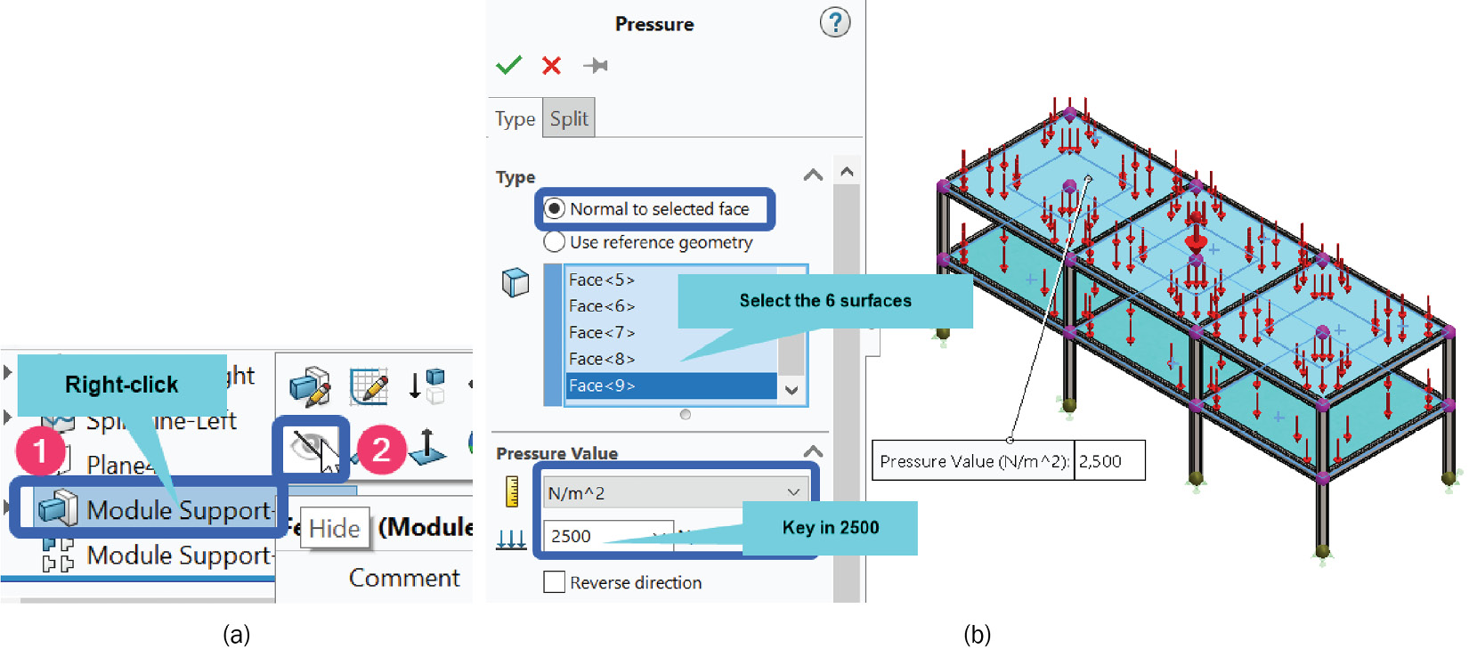
Figure 7.38 – Preparation for the surface pressure application

The last load to be applied is the one acting on the support structures. For this, follow the next steps to apply the pressure loads:

1. First, ensure the support structures are unhidden in the feature manager design tree.
2. Next, right-click on External Loads, select Pressure, then follow the options indicated in Figure 7.39.

Figure 7.39 – Application of the pressure load on the support

Put together, we have now completed the assignment of material properties to all bodies and ensured the fixtures and the loads are applied. We have also assigned thickness to the surface bodies and imposed an interaction/contact condition between selected entities (in addition to the global bonded interaction definition). We are now set to pursue the crucial meshing operations in the next section.

Meshing

The partial view of the simulation study tree shown in Figure 7.40 implies that we have a combination of surface bodies, solid bodies, and beams. As a result, the discretization will comprise shell elements, solid elements, and beam elements.

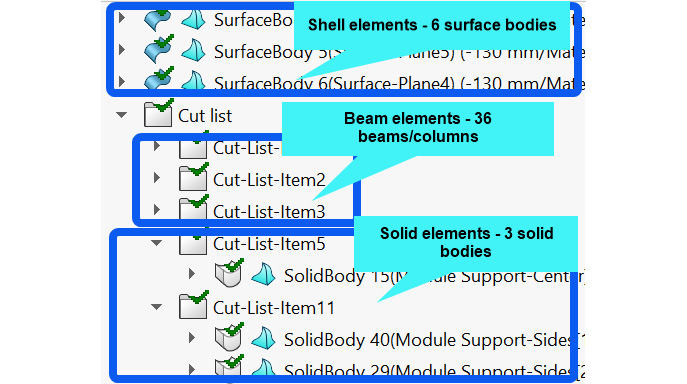
Figure 7.40 – A combination of surface, beam, and solid bodies

Similar to our approach for case study 1, we shall first create mesh control for each family of elements. Afterward, we will generate the mesh. The steps to create the mesh controls for each family of bodies are outlined as follows.

Here are the steps for the mesh control for the beam elements:

1. Right-click on Mesh, then select Apply Mesh Control.
2. From the Mesh Control property manager that appears, under Selected Entities, activate the beam option, then follow the instructions in Figure 7.41.

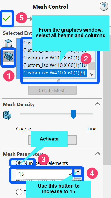
Figure 7.41 – Mesh Control options for the beams

Notice that we are again instructing the meshing engine to discretize each beam/column with 15 beam elements. The simulation study tree should now appear as depicted in Figure 7.42:

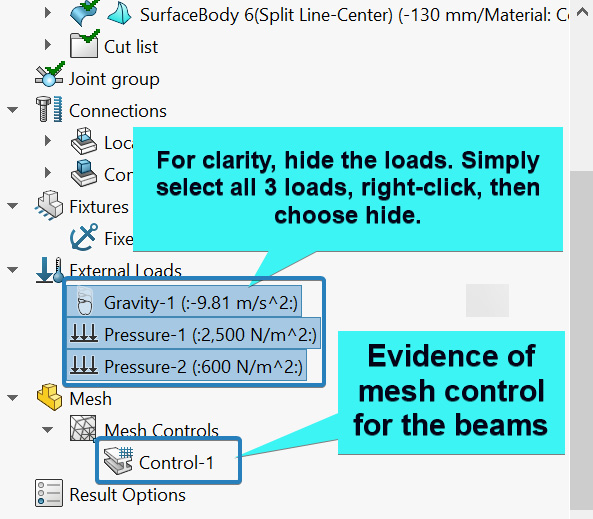
Figure 7.42 – Updated view of the simulation study tree

Here are the steps for the mesh control for the solar supports:

1. If hidden, then unhide the solar modules' support from the feature manager design tree.
2. Next, implement the Mesh Control as illustrated in Figure 7.43.

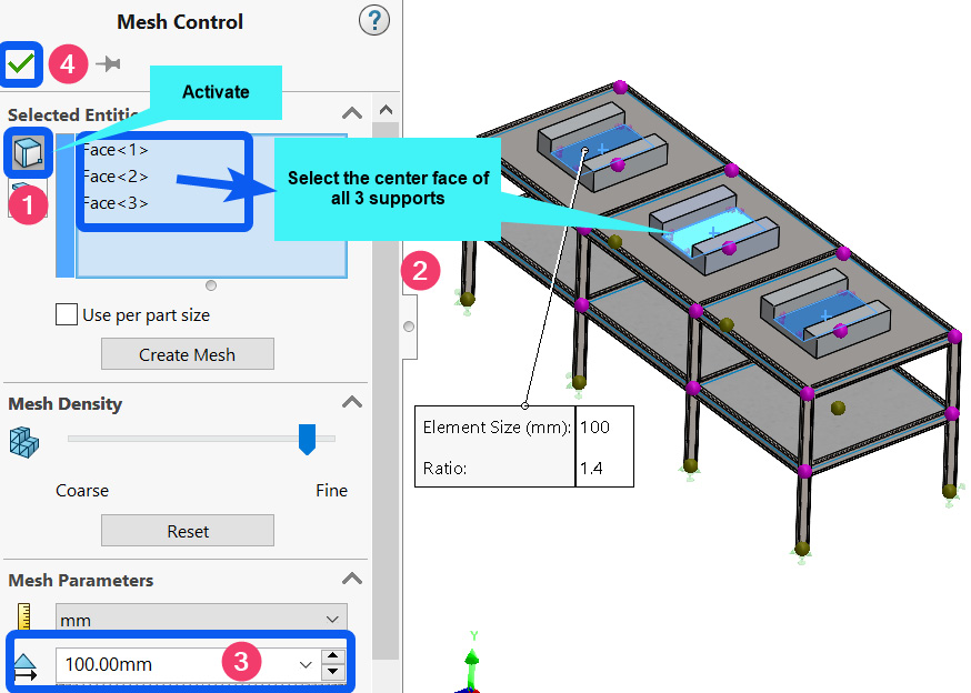
Figure 7.43 – Mesh control for the support structures

With the mesh control specifications accomplished, you should check the simulation study tree to ensure the presence of the controls as indicated in Figure 7.44.

Figure 7.44 – The two mesh controls

Note that each of the mesh control definitions can be examined by simply right-clicking, through which you can also choose to work with the Edit Definition, Details, Hide/Show options, and so on. The Hide/Show option is especially useful to prevent overcrowding the model details in the graphics window. For instance, Figure 7.45 reflects the difference between showing and hiding the mesh controls.

Figure 7.45 – (a) Effect of showing the mesh controls; (b) Effect of hiding the mesh controls

Note that a similar option (that is, Hide/Show) is available for the external loads and fixtures as well. Indeed, the symbols for all three loads that we have applied early on have been hidden to facilitate a neat graphics window (as indicated in Figure 7.42).

With the three meshing controls defined, let's now create the mesh by following the steps highlighted next:

1. Right-click on Mesh, then select Create Mesh.
2. From the Mesh property manager that pops up, increase the fineness of the mesh using the Mesh Factor button as shown in Figure 7.46a.
3. Accept the other default options and click OK.

   After the meshing is complete, the discretized structure should appear as shown in Figure 7.46b.

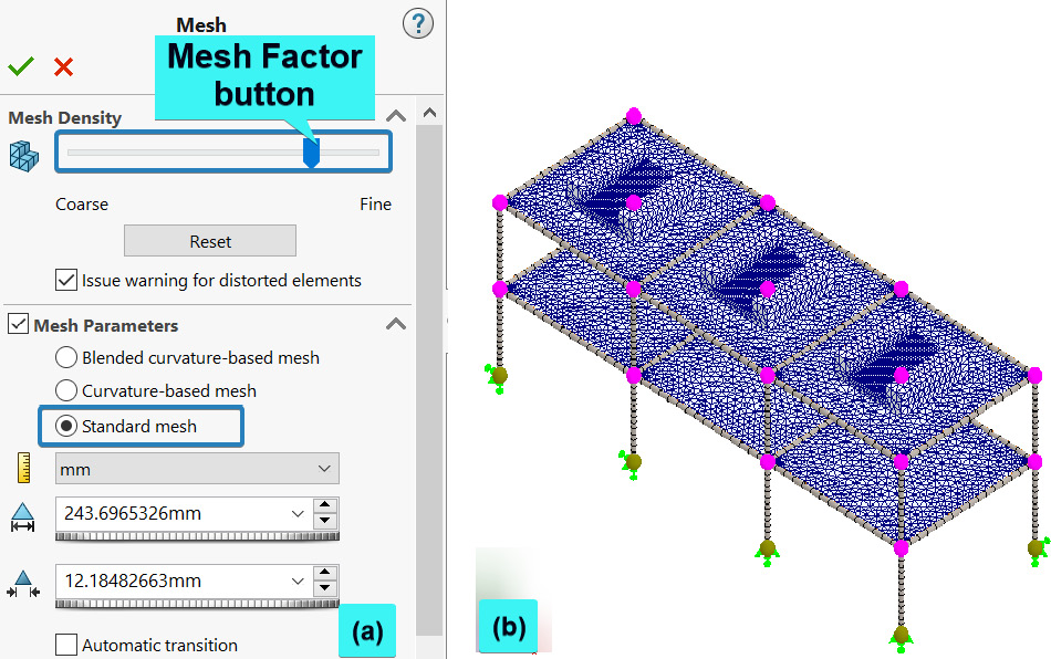
Figure 7.46 – (a) The mesh property manager; (b) View of the meshed structure

We are now poised to run the analysis and retrieve the desired results.

Running the analysis and post-process

Throughout the previous chapters (including the first case study), we have always taken the running of the analysis to be straightforward by accepting the default running properties. But for the current case study, we need to handle things a bit differently for the following reasons:

• First, we have contact interaction (previously known as no penetration contact) between the solar supports and the concrete slabs. A contact interaction is essentially a non-linear interaction condition that will often elongate the duration of the simulation.
• Second, given that the solar modules' support structures are not considered bonded to the surface of the slabs, they may slide or experience a rigid body motion when loads act upon them. Consequently, to prevent this rigid body motion, we shall use one of the SOLIDWORKS Simulation features called soft springs.

To address the issues raised above, we shall now carry out the following steps:

1. Right-click on the analysis/study name, then select Properties... as shown in Figure 7.47.
   

   Figure 7.47 – Activating the study property manager

2. From the static study property manager that appears, under Solver, ensure the Selection option is set to Automatic (labeled 1 in Figure 7.48).
3. Next, check the Use soft spring to stabilize model option (labeled 2 in Figure 7.48).
4. Click OK to close the static study property manager.
   

   Figure 7.48 – Changing the solver and activating the use of soft spring

5. Finally, after the manager window is closed, right-click again on the study name, then select Run as depicted in Figure 7.49.
   

Figure 7.49 – Running the analysis

By monitoring the status of the running process, you will see that it takes a significantly longer time to complete the process than any of the case studies we have studied so far. In any case, after the completion of the running process, we are now set to see what the results tell us about the response of the structure. Our major interests are as follows:

• The new value of the maximum vertical deflection of the concrete slabs
• The changes to the bending stresses of the beams/columns

Obtaining the vertical deflection of the building

Obtain the vertical displacement of the building by following these steps:

1. Navigate to the feature manager to hide the solar modules' support structures (similar to Figure 7.38a).
2. Next, right-click on Results, then select Define Displacement Plot.
3. From the Displacement plot property manager that appears, under the Definition tab, navigate to Display and select UY: Y Displacement.
   

   Figure 7.50 – Options to retrieve the slabs' vertical displacement

4. Update the other usual options by referring to the pictorial guide in Figure 7.50b.
5. Click OK to finish off the selections.

By completing steps 1–4, the plot of the distribution and pattern of the deformation of the slabs along the direction of the Y-axis is revealed as depicted in Figure 7.51.

Figure 7.51 – The new plot of the vertical deflection (with the solar supports hidden)

Figure 7.51 suggests that the addition of the three 3 m by 3 m solar collectors leads to a maximum vertical deflection of -13.676 mm. This represents more than a 70% increase in the vertical deformation of the slab compared to case study 1. While the value of 600 N/m2 pressure imposed on the solar supports represents an approximate hypothetical value, this case study highlights the significant effect that external add-ons acting as a dead load can have on the response of such a structure.

Oftentimes, the serviceability criteria for beams supporting floors have to be checked as well. Hence, it is recommended that you explore the deformations of the beams and columns. In the next sub-section, we shall take a look at the bending stresses that develop in the beams and compare the values to what we obtained in the first case study.

Extracting the stresses in the components

Retrieve the bending stress along direction 1 by following the steps described next:

1. Right-click on the Results folder, then select Define Stress plot.
2. Within the Stress plot property manager that appears, under Display, activate the Beams option (if need be, see the pictorial guide in Figure 7.23) and select Bending in DIR 1.
3. Now, move to the Chart Options tab. Under Position/Format, change the number format to floating.
4. Click OK.

In response to the completion of steps 1–4, the stress plot is displayed as depicted in Figure 7.52, from where it is seen that the bending stresses along direction 1 (X-axis) are now about -59 MPa/+59 MPa. While these values are still well below the yield strength of ASTM 36 steel, from which the members are made, they represent about a 50% increase in the stress along direction 1 reported for case study 1.

Figure 7.52 – The deformed shape of the beams for the bending stress along the X-axis (case study 2)

Repeat steps 1–4 to examine the stress along direction 2 by choosing Bending in DIR 2. The result is presented in Figure 7.53.

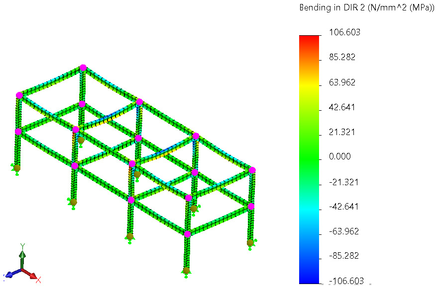
Figure 7.53 – The deformed shape of the beams for the bending stress along the Z-axis (case study 2)

As you can see in Figure 7.53, the maximum compressive and tensile bending stresses in the members are now -106 MPa/+106 MPa. This is also about 50% higher than was reported for case study 1.

This ends our exploration of the second case study and marks the end of this chapter. In tackling the two simulation studies, we have harnessed a few more features of SOLIDWORKS Simulation. Like the other chapters, there are far more results that we could obtain from the simulation studies. It is hoped that you have gained a foundation to go deeper and check some of these other results. For instance, the factor of safety of the beams/columns, the factor of safety of the slabs, the strains and stresses in the slabs, and so on.

Summary

We have explored two examples within this chapter that allowed us to walk through simulations with mixed elements. Via these case studies, we have demonstrated the following:

• How to handle local mesh control for each family of elements in a mixed element analysis
• How to create a custom material from scratch and apply gravity load
• How to define a no penetration contact set between solid and shell bodies
• How to use the automatic contact pair detection tool
• How to update a study property to select a solver and employ the in-built soft spring to stabilize a structure

In the next chapter, we will examine the analysis of components with advanced materials in the form of composites.

Exercises

1. Repeat case study 2 by replacing the contact local interaction with a bonded local interaction, in addition to the global bonded interaction. What effect does this have on the running of the simulation, the deformation, and the stress distributions?
2. Repeat case study 2 for a situation where the thickness of the concrete slabs at the top is changed to 160 mm, and those at the bottom changed to 100 mm. Re-conduct the simulation without the use of the soft spring option. Explain how these changes affect the simulation running behavior, the deformation, and stress distributions.

Further reading

• [1] Simulation - Mixed Mesh Techniques, S. Solutions, ed, 2019, pp. https://www.solidsolutions.ie/solidworks-videos/simulation-mixed-mesh-techniques.aspx.
• [2] H. H. Lee, Finite Element Simulations with ANSYS Workbench 17, SDC Publications, 2017.
• [3] Design Loads for Residential Buildings, US, 2000 [Online]. Available: https://www.huduser.gov/publications/pdf/res2000_2.pdf
• [4] An Introduction to Soil Mechanics, A. Verruijt, Springer International Publishing, 2017.
• [5] Design, construction and performance prediction of integrated solar roof collectors using finite element analysis, M. M. Hassan and Y. Beliveau, Construction and Building Materials, vol. 21, no. 5, pp. 1069-1078, 2007.
• [6] Performance evaluation and techno-economic analysis of a novel building integrated PV/T roof collector: An experimental validation, B. Mempouo, and S. B. Riffat, M. S. Buker, Energy and Buildings, Vol. 76, pp. 164-175, 2014.