Chapter 2: Analyses of Bars and Trusses

This chapter demonstrates the SOLIDWORKS simulation procedure for structures that primarily support axial loads. The simplest form of this type of structure is known as bars or rods. In the more complex form, they are known as plane and space trusses (which are just the two-dimensional and three-dimensional arrangements of bars, respectively). By the end of this chapter, you will be familiar with the procedure for the simulation of the aforementioned structures. Against this backdrop, the focus of this chapter is anchored on the following topics:

• Overview of static analysis of trusses
• Strategies for the analysis of trusses
• Getting started with truss analysis via SOLIDWORKS Simulation

Technical requirement

You will need to have access to the SOLIDWORKS software with a SOLIDWORKS Simulation license.

You can find the sample files of the models required for this chapter here: https://github.com/PacktPublishing/Practical-Finite-Element-Simulations-with-SOLIDWORKS-2022/tree/main/Chapter02

Overview of static analysis of trusses

This section provides basic background information about bars and trusses. It highlights the objectives of analyzing these structures and their applications.

Let’s start with some basic definitions. A bar is a structure that is designed to support simple forces along its axis (such as tensile and compressive loads). On the other hand, a truss represents a collection of bars that are arranged as one or more units of triangulated frameworks. Discussions on the analysis of either of these types of structure (that is, a bar or a truss) often deserve separate standalone chapters. Nonetheless, since the analysis of bars is simpler than that of trusses, we shall allocate more time to the simulation of trusses with the understanding that the same knowledge carries over to the analysis of simple bars.

Note

Within the subject of mechanics, a structure broadly refers to a body or a collection of bodies designed to carry loads. Most structures are three-dimensional (3D) in nature. But for ease of analysis, engineers often leverage approximations that facilitate the use of one-dimensional (1D) members (such as a bar, a shaft, a beam, a column, and so on) or two-dimensional (2D) approximations (such as plates and shells, and so on) to reduce the computational burden of complex 3D analyses.

You will have seen the application of truss structures in various forms around you. Some of these are shown in Figure 2.1. Typically, truss structures are featured prominently in the design of cranes, truss booms, telecommunication towers, masts, electric pylons, roofs, bridges, and so on.

From an engineering performance analysis point of view, we conduct static analyses of bars and trusses with the following objectives:

• Determining the internal forces and consequently the stresses that developed in the members
• Evaluating the axial deformation, the members experienced upon loading

In bars and trusses, the axial deformations manifest in the form of shortening (contraction) or lengthening (extension) of a member’s length. Consequently, a combination of compressive and tensile normal strains/stresses develops in these structures. Together, the stress and the deformation data that we retrieve from simulations help in determining the right geometric sizing for the members (called proportioning). But crucially, the results contribute towards our ability to design these structures to hedge against unwanted failure or excessive deformation during in-service usage. For brevity, in the rest of this chapter, we shall be using the term truss as a shorthand for axially loaded structures.

Figure 2.1 – Some applications of trusses in practice

Before we get deep into analysis, it is important to be aware of the following technical points that are frequently considered for the computer analysis of trusses:

• The members of a truss are straight and have uniform cross-sections.
• The ends of an individual member of the truss are connected to the ends of other members at joints via frictionless pins. In practical scenarios, such joints may be formed by rivets/bolts/ball and socket joints or via welding to a gusset plate.
• Forces and supports are applied only at the joints of a truss.

With the background information provided about trusses, let’s now take a look at strategies for their simulations in the next section.

Strategies for the analysis of trusses

This section describes the structural details and the modeling strategies for the simulation of truss structures. It also highlights the major features of the truss element within the SOLIDWORKS Simulation library.

Structural details

Trusses can be designed to function under a wide spectrum of load-supporting applications. However, irrespective of what form they take in appearance, a consistent set of parameters is employed for their analyses. This implies that irrespective of the form of the truss you are analyzing, you will need to know the following technical information before venturing into the analysis:

• The dimensions of the truss:
  1. The details of the cross-section
  2. The geometric length of each member
  3. The orientation angles of the members
• The material properties of the truss members
• The loads applied to specific joints of the truss
• The support provided to the truss to prevent rigid body motion

  Note

  In practice, a chunk of time will be spent spelling out the scope of the problem relating to structures’/products’ design and analyses. Things such as what the magnitude of the load should be. In what environment will the truss be used? What materials should be used? What types of support are required? What dimensions should be assigned to each member? And so on. In short, to achieve meaningful simulation results, attention should be paid to project specifications and parameters before commencing the simulation tasks. That said, for much of this book, these details will be provided so we can focus squarely on the simulation tasks without getting bogged down by the time-consuming iterative conceptual design tasks.

Modeling strategy

When we analyze truss structures via the finite element simulation method, a basic strategy is to take a structure such as that in Figure 2.2 (a), split it into its constituent members (Figure 2.2 (b)), and then treat each member as a truss element. So, in the end, a whole structure formed from the assembly of different members is represented by the collective behavior of individual truss elements.

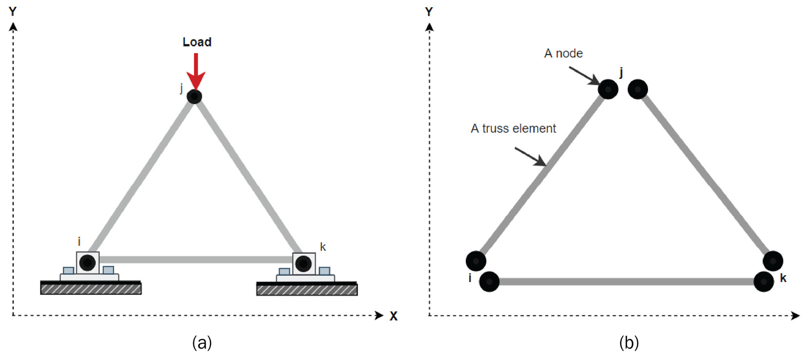
Figure 2.2 – (a) Illustration of a simple truss structure; (b) splitting the structure into elements

Figure 2.3 illustrates the other aspect of the strategy for the simulation of trusses:

1. The first step is modeling the skeletal arrangement of the truss or a collection of bars within the SOLIDWORKS model environment.
2. This is then followed by the conversion of the skeletal model into a weldment profile, transforming the weldment model into a finite element model.
3. Finally, run the analysis to obtain the results (within the SOLIDWORKS Simulation window).

Figure 2.3 – Major steps in the static analysis of trusses

Characteristics of the truss element in the SOLIDWORKS Simulation library

In the traditional theoretical treatment of the finite element simulation method, the truss element is generally known to be a plane element with two nodes and two degrees of freedom. Within the SOLIDWORKS Simulation environment, the truss element is a 3D two-node element with three degrees of freedom per node (that is, translational displacements about the x, y, and z axes). The beauty of the 3D truss element in SOLIDWORKS is that it can be used to analyze 1D bars, 2D plane trusses, and 3D space trusses.

We will go through a case study in the next section to explore further details about the simulation of a loaded truss structure.

Getting started with truss analysis via SOLIDWORKS Simulation

In this section, we will demonstrate the use of the truss element with a practical case study. Primarily, we will analyze the structural performance of a crane used in the spatial positioning of heavy objects on a mega building construction site. The example is inspired by exercise 4.11 in the textbook by Megson [1] (see the Further reading section). It is a practical problem that can only be solved satisfactorily via computer analysis.

Time for action – Conducting static analysis on a crane

Problem statement

Consider the 2D representation of a crane shown in Figure 2.4, which is to be analyzed based on the placement of 1500 kN and 2000kN weights at points R and W, respectively.

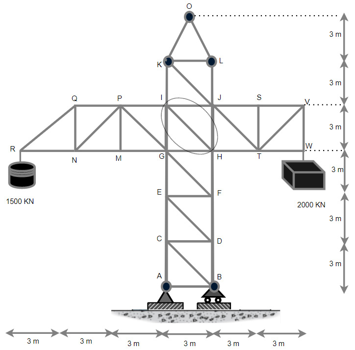
Figure 2.4 – A 2D schematic of a crane

For convenience, we shall consider that the members of the crane are derived from tubular alloy steel. For this material, the Young’s modulus, E, is taken as 210 GPa. The members have the same cross-sectional detail characterized by external and internal diameters 200 mm and 80 mm, respectively. Using SOLIDWORKS simulation, we want to answer the following questions:

• What is the maximum resultant deformation of the truss upon the application of the loads?
• What is the distribution of the factor of safety of the members of the crane upon loading?
• What is the internal force/stress that developed in the member IH?

Part A – Creating the sketch of the geometric model

The first step in any analysis is to have a model of the structure to be analyzed. This section centers around the creation of the basic geometric lines describing the structure.

Starting up the SOLIDWORKS interface

To create the skeletal sketch of the model, launch SOLIDWORKS and follow these steps:

1. Click File.
2. Select New.

   After step 2, the New SOLIDWORKS Document screen appears. We are interested in creating the model using the Part modeling environment.

3. Select Part and then click OK (Figure 2.5).

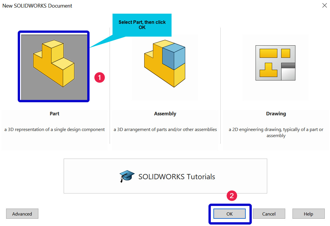
Figure 2.5 – Creating a new Part document

The SOLIDWORKS user interface opens up and we can start sketching right away. But before that, it is a good idea to ensure you are using the right unit of measurement.

Setting the dimensions

Look at the lower-right corner of the graphical user interface (GUI) to ensure that the current unit of measurement is the MMGS (millimeter, gram, and second) system of units, as shown in Figure 2.6.

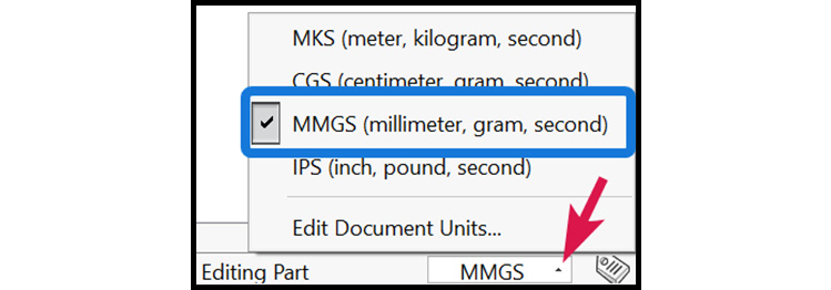
Figure 2.6 – Setting the unit of the document

Once it is confirmed that the right unit is set up, you may save the file as Crane.

Sketching the lines describing the geometry of the crane

The view of the crane shown with the problem statement represents the front view. Consequently, we shall sketch the geometric model of the truss on the front plane:

1. Click on the Sketch tab.
2. Click the Sketch manager, as shown in the following figure.
3. Choose Front Plane.
   

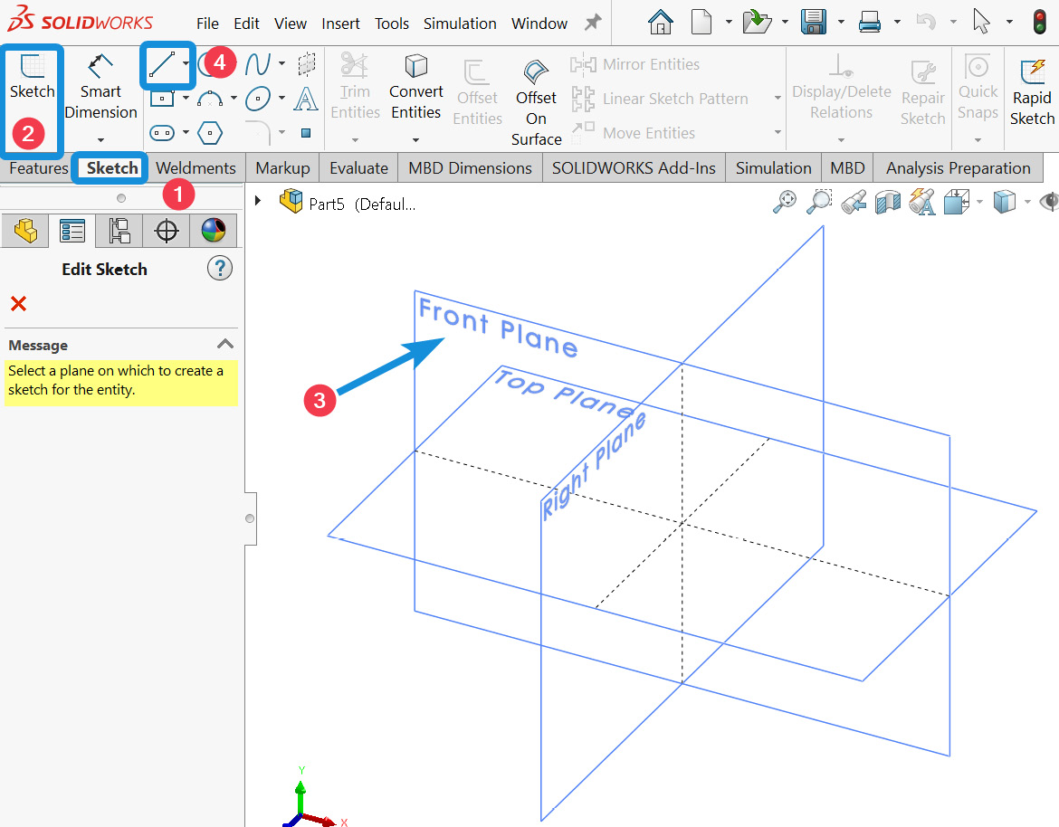
   Figure 2.7 – Commencing the sketching task

4. Create the sketch of the crane with the line sketching tool. Ensure the sketch is symmetric around the origin (coordinate 0 of the graphics window), as shown in Figure 2.8.
5. Save and exit from the sketch. Note the symbol for exiting the sketch shown in Figure 2.8.

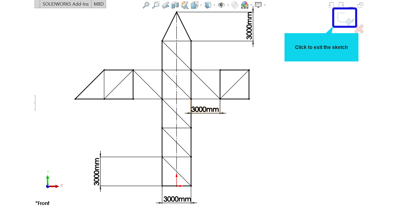
Figure 2.8 – A line-based geometric model of the crane

After completing the sketch, it should look as in the screenshot shown in Figure 2.8. Now, the sketch we have created in this section is just a series of lines with no volume property. As such, it cannot be used for structural analyses. In the next section, we will convert the sketched line-based model into a structural model with a volume property.

Part B – Converting the skeletal model into a structural profile

This section explains how to convert the line sketches we created in the preceding section into a structural model using a special functionality in SOLIDWORKS called the weldments tool.

Introducing the weldments tool

The weldments tool in SOLIDWORKS makes it easy to prescribe the cross-sectional details for sketched lines. In other words, it facilitates the transformation of lines with no volume properties into structural members with volume properties that are suitable for realistic engineering simulation.

The weldments tool can be used with both 2D and 3D sketches. What is more interesting about this tool is that it provides us with access to a handful of relevant structural profiles, such as those listed in Table 2.1.

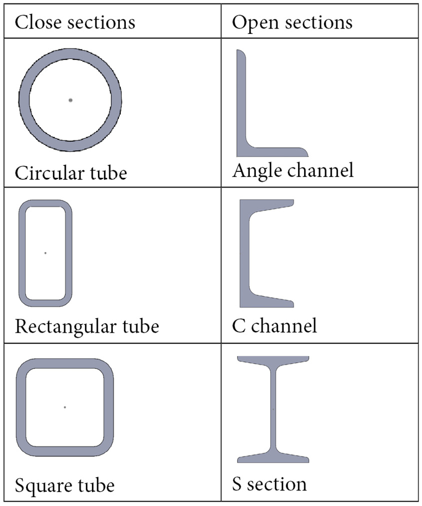
Table 2.1 – Samples of in-built structural cross-sections in the weldment library

The profiles highlighted in Table 2.1 are stored in the SOLIDWORKS installation folder. For instance, for laptops/PCs with a Windows operating system, the folder is located at Drive:Program FilesSOLIDWORKS CorpSOLIDWORKSlangenglishweldment profiles.

Note that Drive is a placeholder for the storage drive containing the SOLIDWORKS installation folder on your device. Scrutinizing the aforementioned directory address, you will notice that the profiles are contained in the parent folder named weldment profiles. This folder contains sub-directories, as shown in Figure 2.9 (a). Further, opening any of the sub-directories will expose relevant files with the .sldlfp extension, as shown in Figure 2.9 (b).

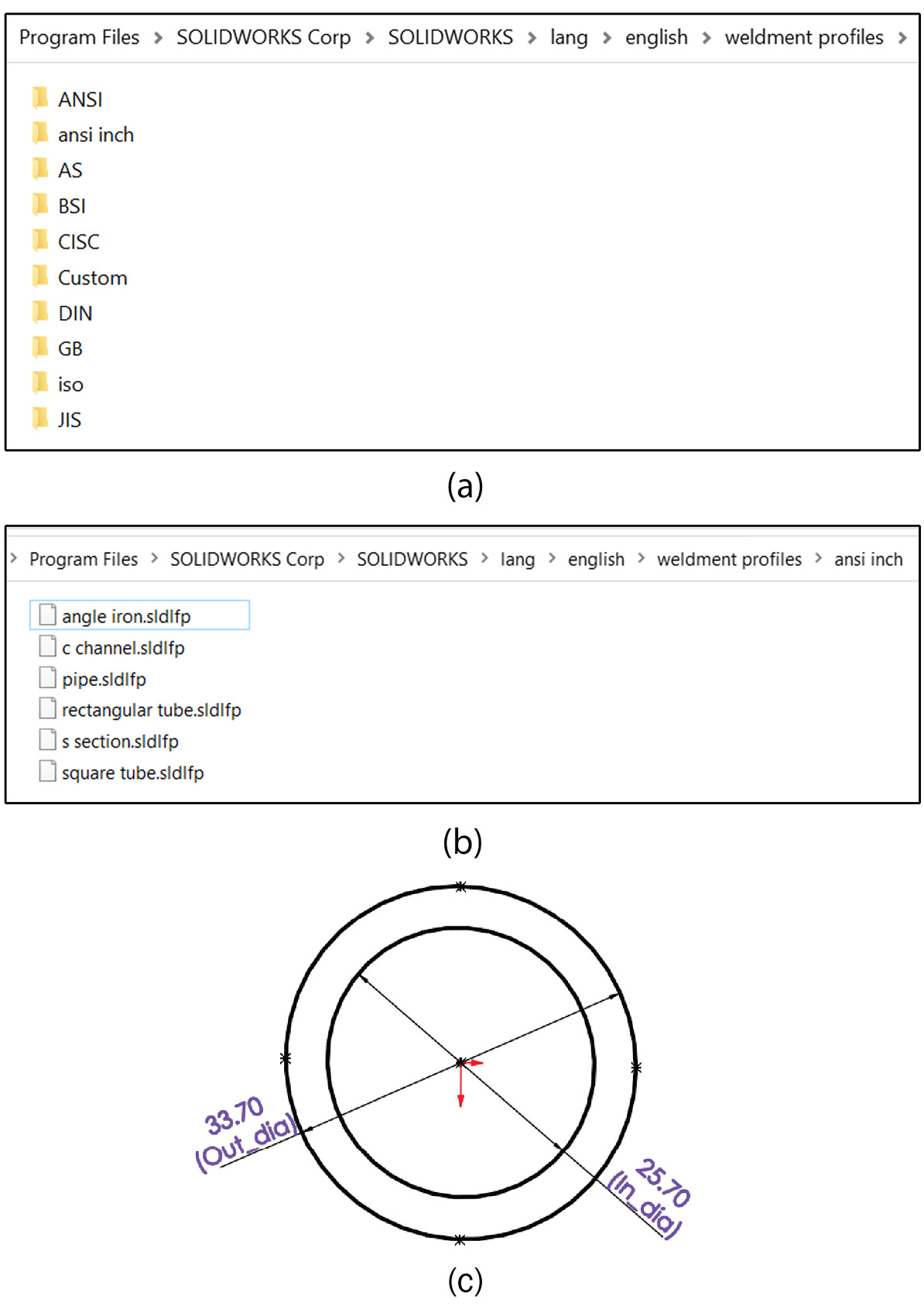
Figure 2.9 – The content of the weldment profiles directory: (a) the two original sub-folders; (b) the library’s six profile files in one of the original folders; (c) the dimensions of the largest ISO tube profile in the weldment library

Now, the profiles that are bundled with the weldments tool have pre-defined dimensions, but these dimensions may differ from what we need. Consequently, it is common to have to adjust or edit these profiles to fit our needs. For instance, the external and internal diameters of the cross-section we need are 200 mm and 80 mm, respectively (from the problem statement). However, the largest tube within the weldment profiles folder differs from these values, as indicated in Figure 2.9(c). In the next sub-section, we will explore how to edit the profile for our needs, but we first need to activate the weldment profile.

Information

Our main interest is in using the weldment tool to supply the cross-sectional details of the members. However, it has many features that can be further explored. Relevant details can be found by following this SOLIDWORKS help link: https://help.solidworks.com/2022/english/SolidWorks/sldworks/c_Weldments_Overview.htm?verRedirect=1.

Activating the weldments tool

Check the set of items in your SOLIDWORKS’s CommandManager tab to see if the Weldments tab is present. If the CommandManager tab is missing the Weldments tab, then follow these steps (summarized in Figure 2.10):

1. Right-click on the CommandManager tab to bring up the option to show more tabs.
2. Move your cursor over the word Tabs.
3. Click on Weldments (this will activate the Weldments tab).

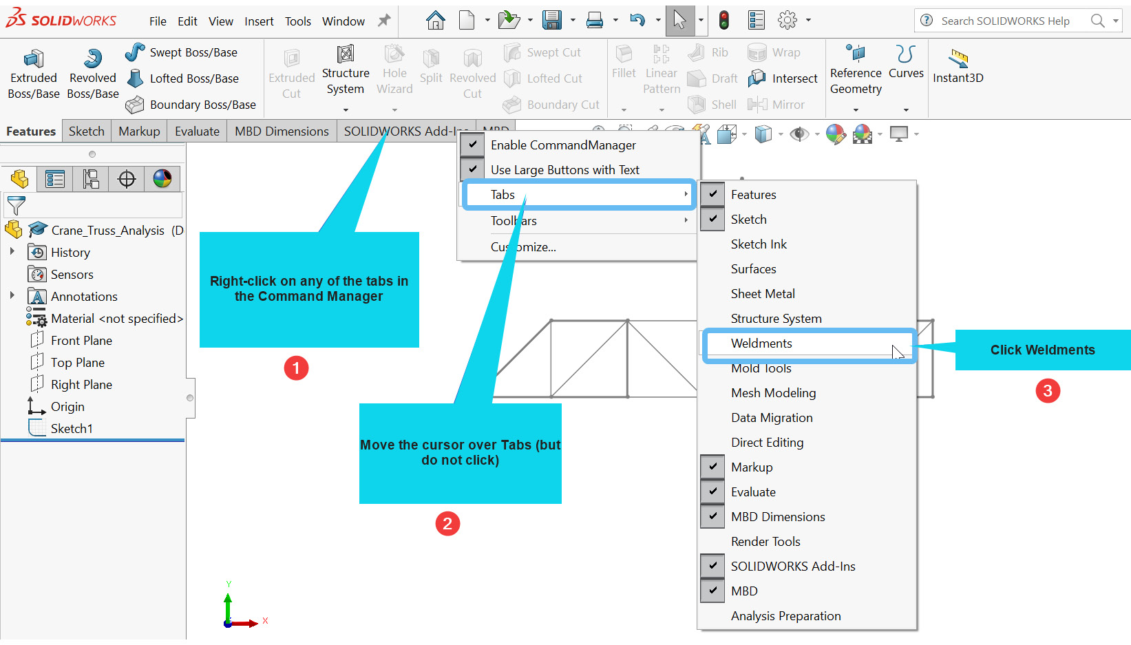
Figure 2.10 – Activating the Weldments tab when it is unavailable under the Command Manager tab

With the Weldments tab on, the next sub-section illustrates how to convert the sketched lines to structural members.

Adding structural properties

Follow these steps to transform the sketched lines into structural members:

1. Click on the Weldments tab (Figure 2.11).
2. Click on Structural Member.
   

   Figure 2.11 – Initiating the conversion of the sketched lines into structural members

   Once you have clicked on the Structural Member command, the Structural Member property manager window will open on the left side of the GUI. Select the options highlighted in Figure 2.12.

3. Under Standard, choose iso.
4. Under Type, select pipe.
5. Under Size, select 33.7 x 4 – this refers to a tube with an external diameter of 33.7 mm and a thickness of 4 mm.
6. Click New Group to form Group 1 and select the lines shown in Figure 2.13a. After completing the selections for Group 1, proceed to form Group 2 by selecting the lines highlighted in Figure 2.13b.
   

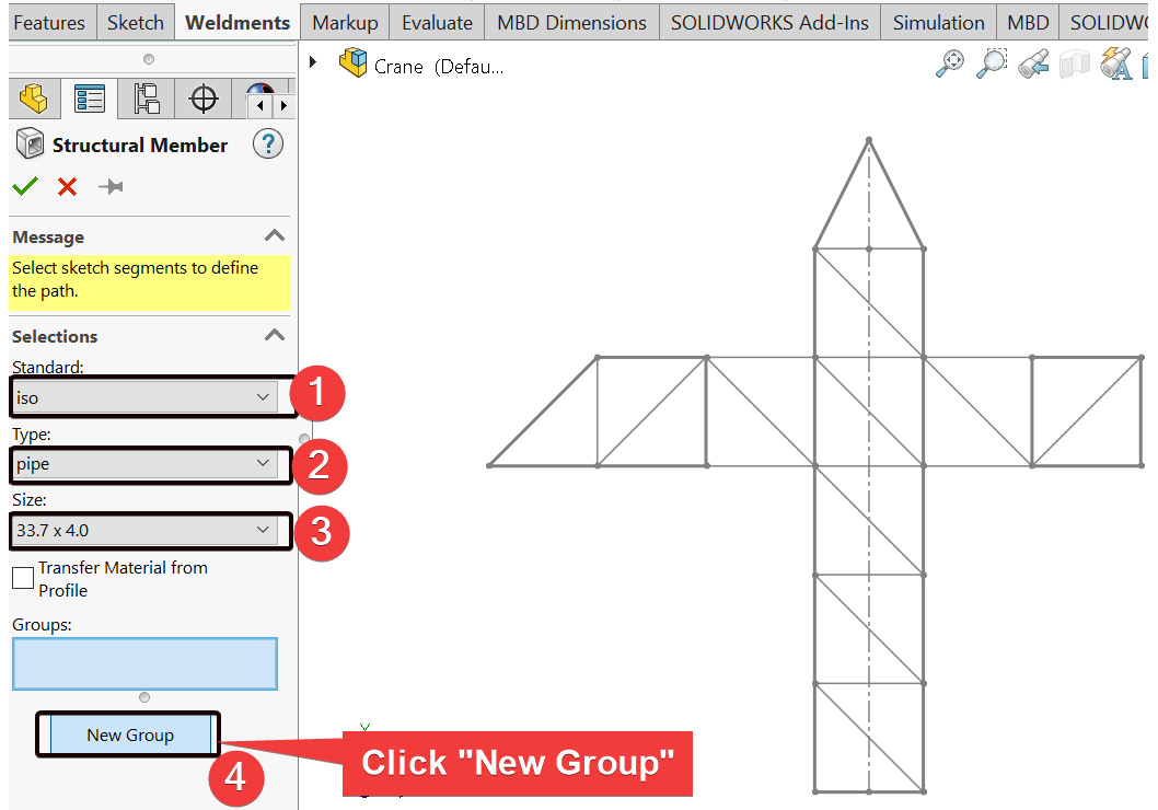
   Figure 2.12 – Specifying options for the profile of the cross-section

   For ease of forming the structural members, Figure 2.13 (a-f) illustrates the series of lines to be selected for each group.

   

   Figure 2.13 – Path segments for the weldment profiles

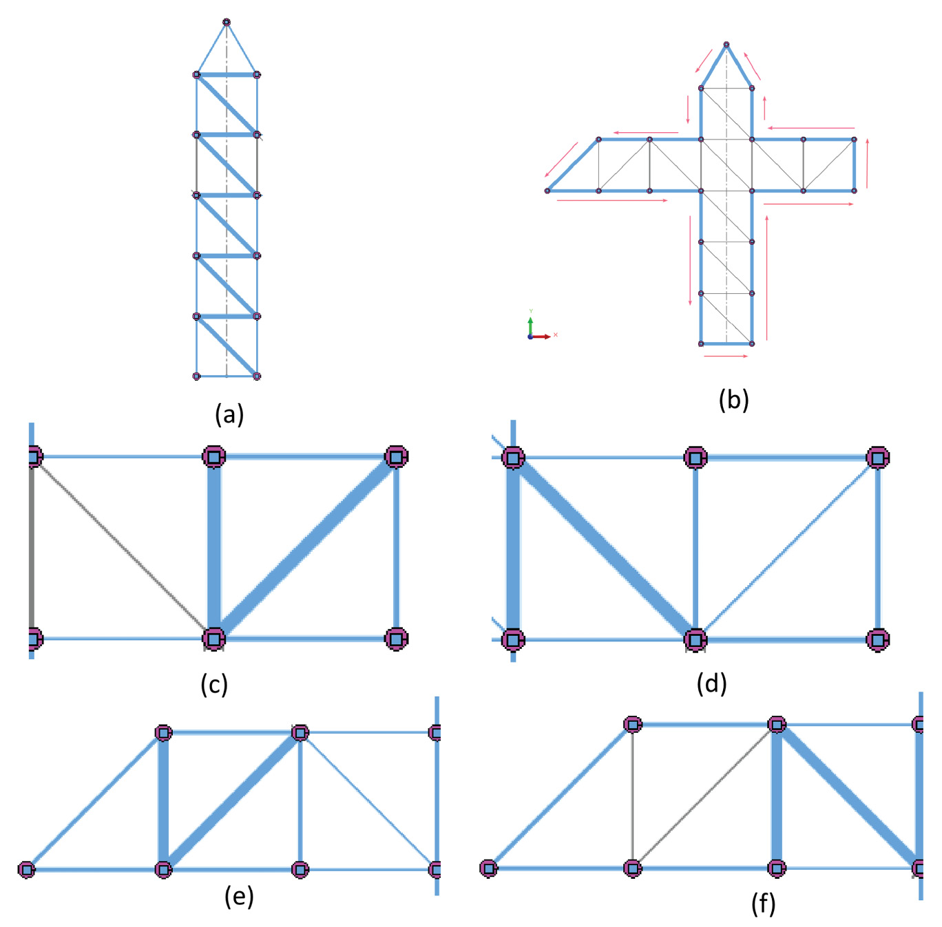
7. Form all the six groups (as indicated in Figure 2.14).
8. Under the settings options, ensure that the Apply corner treatment box is unticked.
9. Click OK.

Figure 2.14 – Finalizing the selection for the cross-section

By completing steps 1-9, the Feature Manager tree will appear with some additional items. Five of these are highlighted in Figure 2.15:

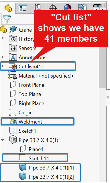
Figure 2.15 – New items within the feature manager

• Cut list (41): In general, this is a folder that contains the details of the weldment items in the current part file. As you can see, it shows that we have a total of 41 weldment items that make up our structure.
• The Weldment symbol. This appears once you click on Structural Member under the Weldments tab.
• The Structural Member symbol: This also appears in response to using the Structural Member command.
• Sketch11: This is the sketch of the cross-section of our weldment profile.
• Pipe: This is the main branch of the collection of extruded bodies representing the 41 structural parts of the crane.

Editing the cross-section for our needs

The cross-section that we have employed from the weldment library is not the same as that stated in our problem statement. Thus, it is necessary to change the dimension of this cross-section to suit our needs. To do this, take the following steps:

1. Right-click on Sketch11 and select Normal To (as shown in Figure 2.16).
2. Right-click again on Sketch11, but this time, select Edit Sketch.
   

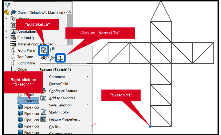
   Figure 2.16 – Steps to edit Sketch11

3. Zoom out so you can see the cross-section, as shown in Figure 2.17a.
4. Edit the sketch to comply with our desired dimensions, as shown in Figure 2.17b.
5. Save and exit the sketching mode, then change the view of the model back to Front View.

Figure 2.17: (a) The original cross-section of the tube; (b) the updated cross-section detail for our analysis

Completing steps 1-5 wraps up the creation of the structural model with a volume property, and we shall next transition to the initiation of the simulation study.

Part C – Creating the Simulation study

In this section, we will activate the Simulation add-ins, specify the material for the members, indicate how to select the truss element, apply fixtures/loads, and finally, initiate the meshing process.

Activating the Simulation tab and creating a new study

Follow these steps to activate the simulation tab and create a new study:

1. Click on SOLIDWORKS Add-Ins.
2. Click on SOLIDWORKS Simulation to activate the Simulation tab.
   

   Figure 2.18 – Activating the SOLIDWORKS add-ins

3. With the Simulation tab active, click on New Study.
   

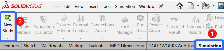
   Figure 2.19 – Creating a new study

4. The preceding step launches the Study property manager (Figure 2.20).
5. Keep the Static analysis option selected by default.
6. Input a study name within the Name box (for example, Crane Analysis).
7. Click OK (this closes the Study property manager panel and launches the Simulation tree).
   

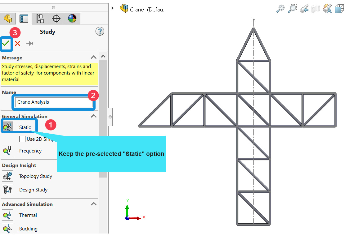
Figure 2.20 – Static study property manager

After completing steps 1-7, you will notice the changes shown in Figure 2.21. Basically, joints will be imposed at the connection points between the members of the truss. At the same time, the Simulation commands will become available:

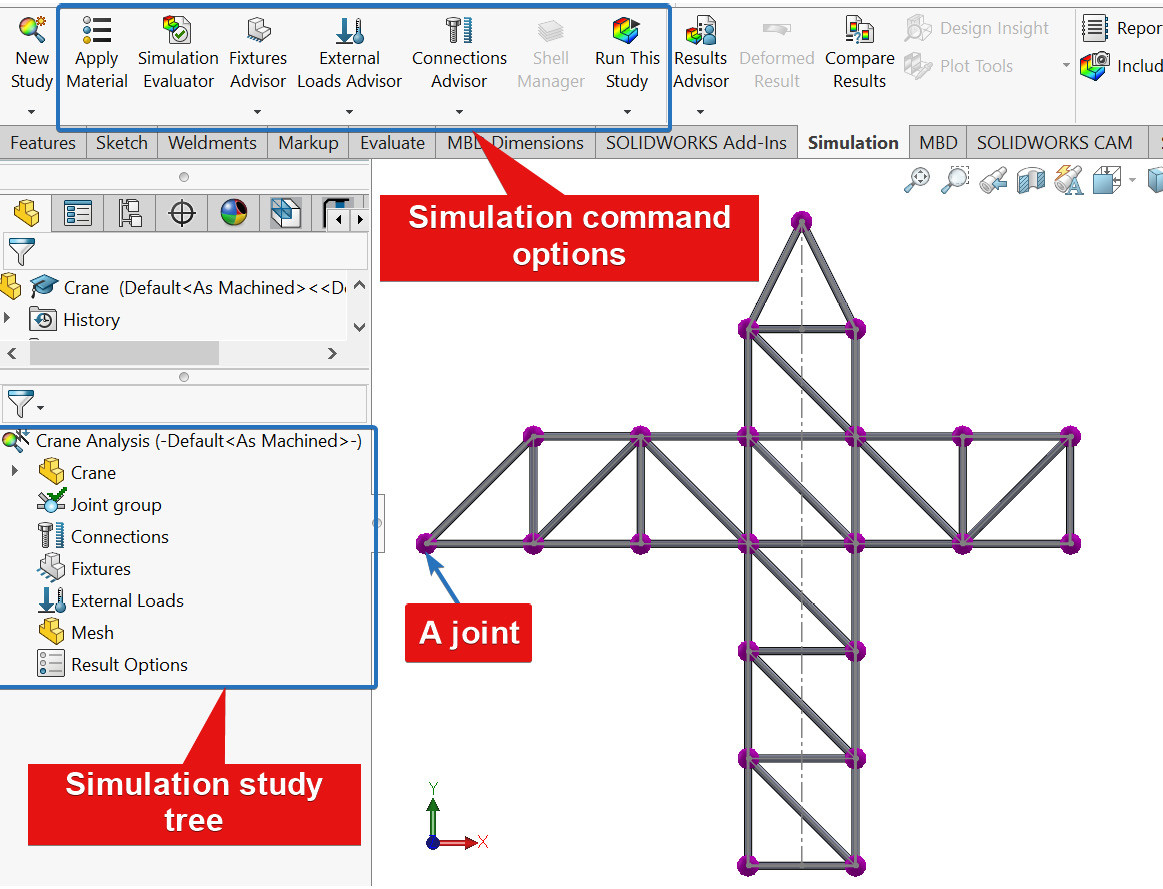
Figure 2.21 – Appearance of joints in the model with the Simulation study tree

In the next sub-section, we will specify the material property for the members.

Adding a material property

Every single member of the crane is assumed to be made of the same material. This makes it easy to apply the material to the members at once:

1. Right-click on the part name – Crane (Figure 2.22).
2. Click Apply Material to All Bodies.
   

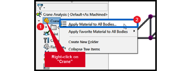
   Figure 2.22 – Activating the material database

   Step 2 launches the material database, which is shown in Figure 2.23. For our analysis, the material that we want is alloy steel, which will be located in the sub-folder called Steel. If necessary, expand the Steel folder, then perform the following steps.

3. Select Alloy Steel.
4. Click Apply.
5. Click Close.
   

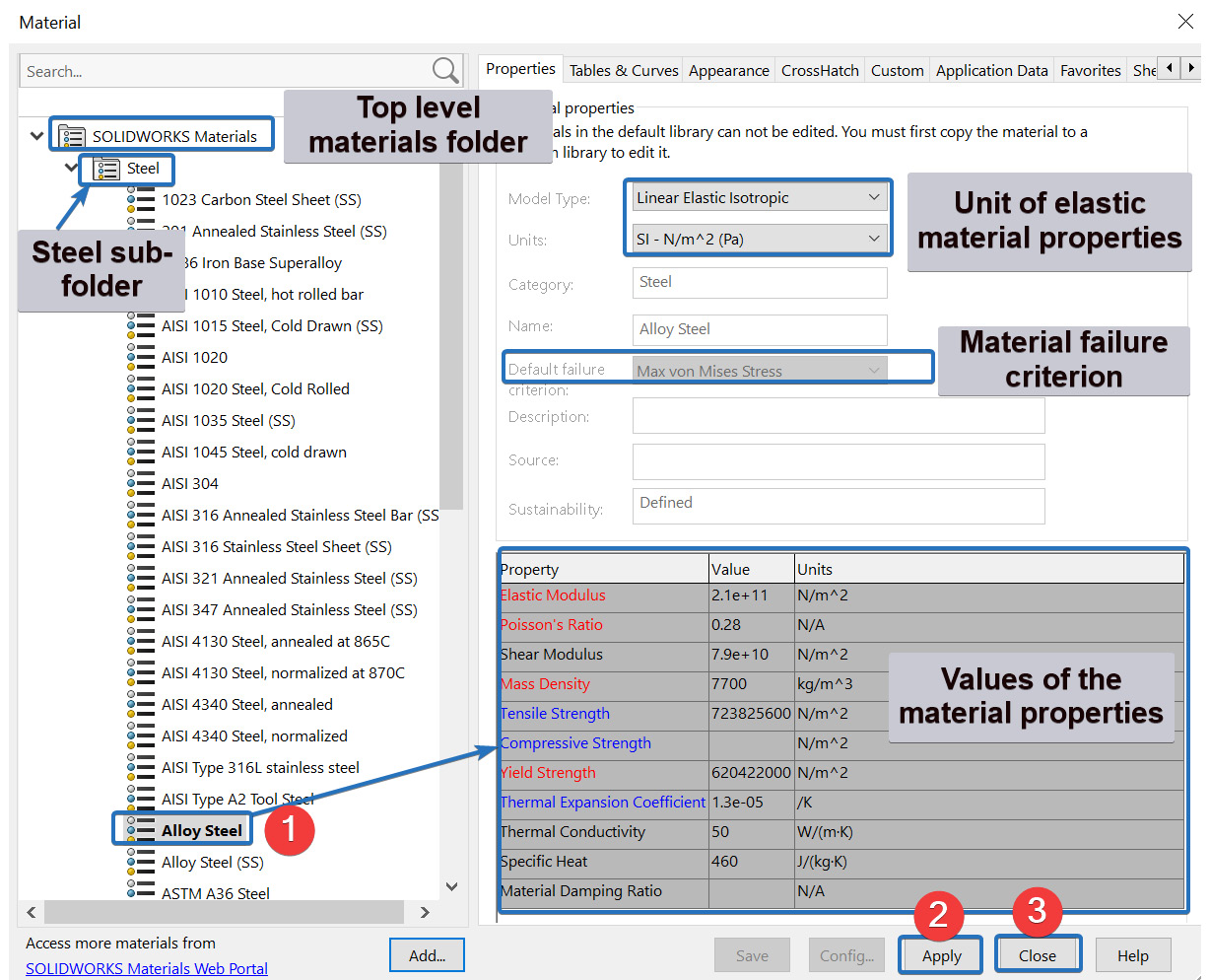
Figure 2.23 – Activating the material database and choosing a material

Before moving to the next sub-section, there are a few features to be observed with the material database. First, the material database is a multilevel directory. At the top layer is SOLIDWORKS Materials, then we have sub-folders that contain the same family of materials, and another sub-folder for custom materials. Second, the material property names in Figure 2.23 are either in black, blue, or red font. In general, the material property names in red font are the ones that are necessary for static analyses. Without values provided for the property names in red font, the simulation will not run. Thirdly, a material failure criterion (Max von Mises Stress) and Linear Elastic Isotropic material model are pre-defined for the selected material. Lastly, after closing the material database window, a green tick mark (ü) will appear on the study name.

Changing from a beam element to a truss element

By default, SOLIDWORKS Simulation treats a structural member that is created using the weldment tool as a beam element during the analysis. However, for our case study, what we need is a truss element. Therefore, in this sub-section, we will convert all the structural members from beams to trusses. To do this, in the simulation tree, do the following:

1. Expand the folder named Cut list – this reveals a set of sub-folders as shown in Figure 2.24 (a).
2. Expand the first sub-folder named PIPE 200 X 4.0.
3. Select all members. Note that this is a long list, Figure 2.24 (b) shows only a partial view.
4. Click Edit Definition.
   

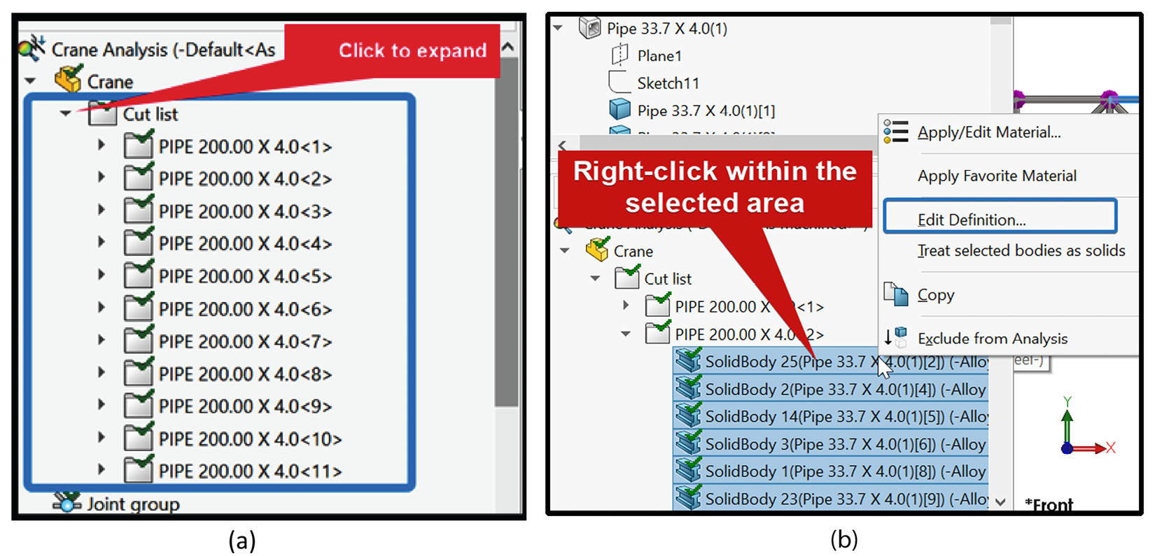
   Figure 2.24 – (a) Revealing the structural member sub-folders; (b) selecting the structural members

5. In the Apply/Edit Beam property manager that appears, select Truss (as shown in Figure 2.25).
6. Click OK.

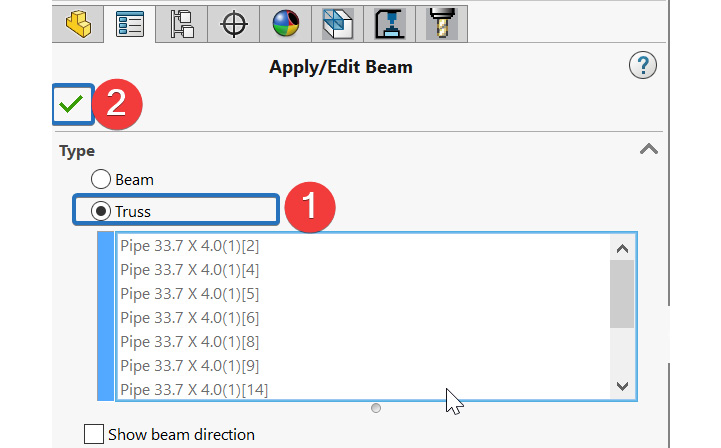
Figure 2.25 – Changing from a beam to a truss

Repeat sub-steps 2-6 for every sub-folders under the Cut list to convert the beams to trusses. After completing the conversion of all members, we can now move on to the next phase, which is about the application of constraints or what we often refer to as boundary conditions.

Applying a fixture

A fixture is a constraint that we apply to structures to restrict the movement of its joint/segment when loads are applied. For this analysis, we will apply three sets of restraints to the structural model of the crane:

• A fixture that will prevent the normal movement to the front view of all the joints (that is the vertices of the crane). This needs to be done because we are running a planar (2D) analysis of the crane. However, if we are running a 3D analysis, this is not necessary.
• A fixture that prevents movements in the horizontal and vertical directions at joint A (because joint A has a fixed support).
• A fixture that prevents the movement along the vertical direction at joint B (because this joint is supported by a roller joint).

Let’s start with the application of the first fixture to all the nodes by following the steps highlighted next.

Applying a fixture to restrain the Z motion of all nodes:

1. Right-click on Fixtures.
2. Pick Fixed Geometry from the context menu that appears (Figure 2.26).
   

   Figure 2.26 – Activating the fixture options

3. Under the Fixture property manager that appears, click Use Reference Geometry (Figure 2.27).
4. Move the cursor into the graphic window and pick all the joints one by one.
5. Click inside the box for the reference plane (labeled 3 in Figure 2.27), expand the feature tree manager, and choose Front Plane.
6. Under Translations, click on the box for Normal to Plane (labeled 4 in Figure 2.27).
7. Click OK.

Figure 2.27 – Options for restraining the movements of all joints normal to the front plane

Steps 1-7 will impose a zero translational movement on all the nodes along the z axis. This ensures that we are doing a plane analysis.

Next, we will apply the restraints at joints A and B, both of which are located at the base of the crane, by following the steps given next.

Applying fixture on nodes A and B:

1. To apply the restraint on joint A, right-click on Fixtures and pick Fixed Geometry. Then do the following:
   1. Under the Fixture property manager that appears, pick Use Reference Geometry.
   2. Move the cursor into the graphic window and pick only joint A.
   3. Choose Front Plane for the reference plane.
   4. Under Translation, click on the arrows of the two boxes labeled 4 and 5 in Figure 2.28 (a).
   5. Click OK.
2. To apply the restraint on joint B, follow the options indicated in Figure 2.28b.

Figure 2.28 – (a) Options for restraining vertical and horizontal movements of joint A; (b) options for restraining vertical movement of joint B

Note that for joint A, we could also use the fixture named Immovable (No translation); it performs the same function as what we did using Use Reference Geometry. For joint B, we restrained the movement along the vertical direction only, which is meant to replicate the behavior of a horizontal roller support.

At this stage, we are done with the application of all fixtures that need to be applied for our analysis. In the next sub-section, we will swing our attention to the specification of loads. This will inch us closer to running the analysis.

Applying external loads

Different types of loads can be used in SOLIDWORKS Simulation. For our analysis, we need to apply what is often referred to as payload weights represented by two vertical forces at joints R and W. We will apply the loads by using the External Loads command under the simulation study tree.

Follow these steps to apply the two forces at joints R and W, create the mesh, and then run the analysis:

1. Right-click External Loads.
2. Select Force (Figure 2.29).
   

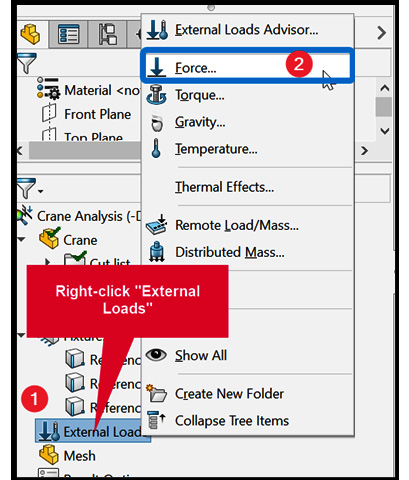
   Figure 2.29 – Beginning the external load’s application

3. From the Force property manager that appears, under Selection, click on the Joints symbol (labeled 1 in Figure 2.30).
4. Navigate to the graphic window and pick joint R (the leftmost joint).
5. Click inside the box labeled 3, then expand the feature manager tree to select Front Plane as the reference plane.
6. Under Units, keep it as SI.
7. Under Force, click in the second force component box (vertical force) and type 1500000.
8. Check Reverse direction (labeled 6 in Figure 2.30). This changes the direction of the force to a downward direction.
9. Click OK.
   

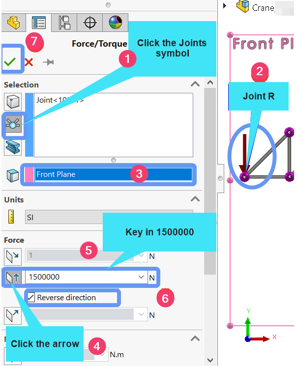
   Figure 2.30 – Selecting the options for applying the force at joint R

10. Repeat steps 1-9 to apply the 2000 kN force on joint W (in step 4, select joint W, and in step 9, key in 2000000).

After completing step 10, the appearance of the model in the graphics window will be as shown in Figure 2.31. The model is displayed in an isometric mode so that the arrows indicating the loads at joints R and W and the fixtures at all joints become apparent.

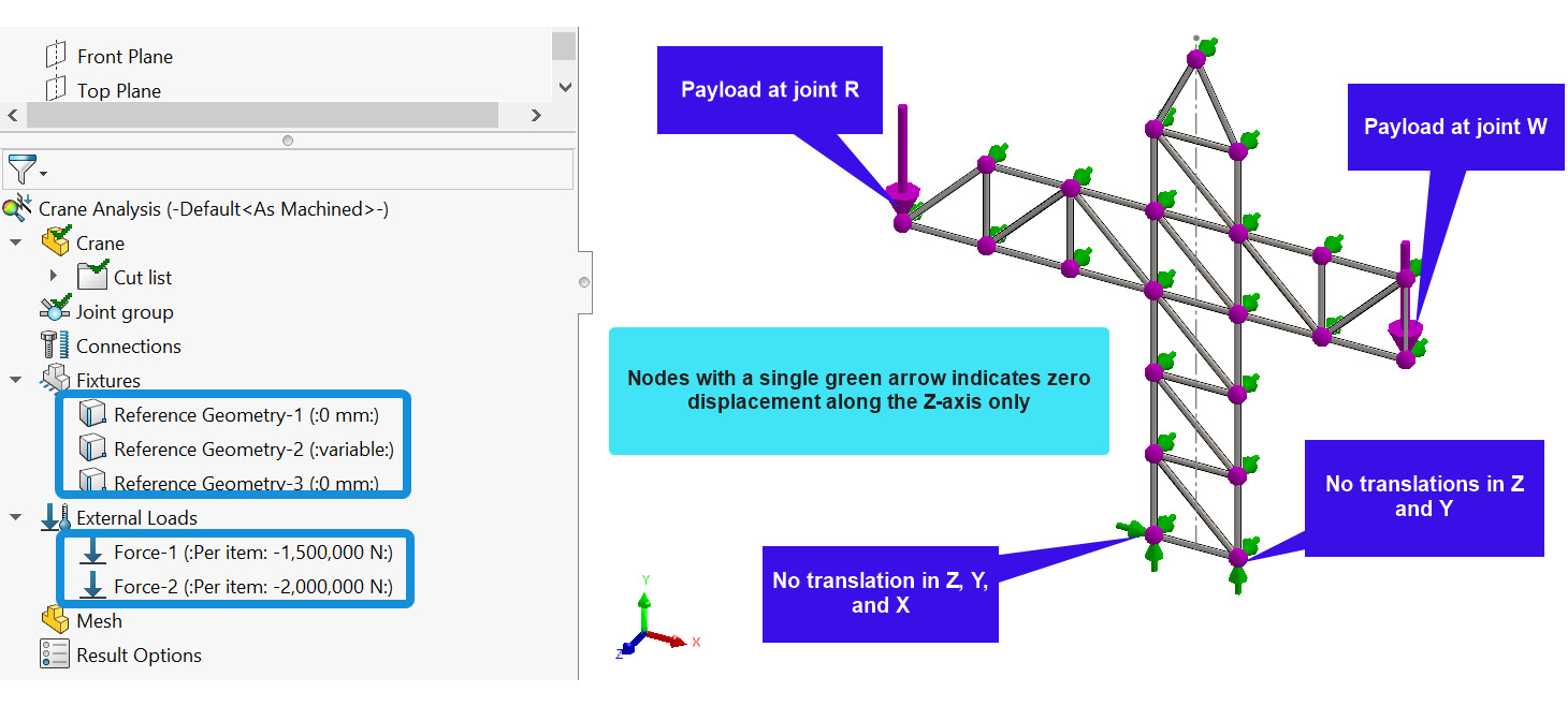
Figure 2.31 – The appearance of the model in the graphics window after applying loads and fixtures

The next task is to mesh and then run the analysis, which is what happens in the next sub-section.

Meshing

Meshing is an essential part of finite element simulation. There are two approaches for creating a mesh in SOLIDWORKS Simulation. The first involves creating the mesh using the command Create Mesh, while the second involves using the command Mesh and Run. For this chapter (as well as Chapter 3, Analyses of Beams and Frames, and Chapter 4, Analyses of Torsionally Loaded Components), we will be using the second approach. Principally, this approach combines the meshing and running of the analysis in a single step, and it works well whenever we use the weldment tool to create the members of a structure to be analyzed. Now, it is good to be aware that SOLIDWORKS does not provide the option for controlling the mesh quality for a structure idealized as a collection of truss elements. This means there is no point in engaging ourselves in the refinement of the mesh that we create for this problem. Further, it means if a truss is made of up 41 members, then only 41 truss elements are sufficient to analyze it accurately. Nonetheless, we will explore meshing in more detail, for instance, in Chapter 5, Analyses of Axisymmetric Bodies, and Chapter 6, Analyses of Components with Solid Elements.

Bearing the aforementioned detail in mind, we can now deal with the last steps before getting our desired results, to this end:

1. Right-click on Mesh.
2. Select Mesh and Run (as indicated in Figure 2.32 (a)).

After completing steps 1 - 2, the study tree will appear as shown in Figure 2.32 (b).

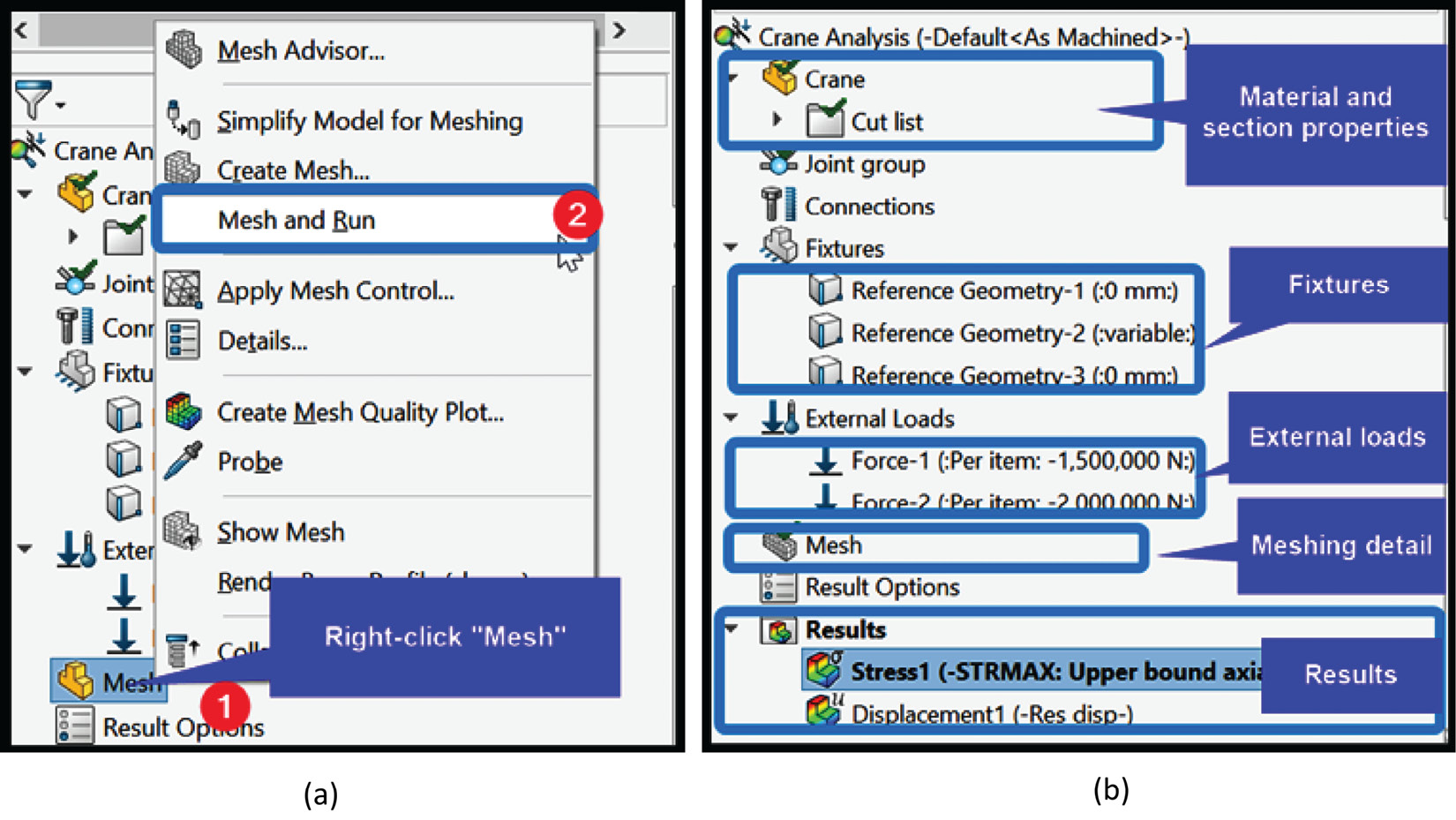
Figure 2.32 – (a) Creating the mesh and running the analysis; (b) Changes in the study tree after the Mesh and Run command

We will examine the results folder further in the next section.

Part D – Scrutinizing the results

Now that we have completed the steps in the previous sections (that is, Parts A-C), we are now in a position to make sense of the results and answer the following questions:

• What is the maximum resultant deformation of the truss upon the application of the loads?
• What is the distribution of the factor of safety of the members of the crane upon loading?
• What is the internal force/stress that developed in the member IH?

But before answering these questions, it is worth noting that by default, when you use SOLIDWORKS for static studies, it generally computes, among others, the Displacements at the joints or nodes of the structure, the Reaction forces at the points of supports, the Strains/Stresses on an element/at the nodes, the Factor of safety, and so on.

Nevertheless, SOLIDWORKS Simulation will not always display all results. In fact, in most cases, the default results may not be what you want (you may simply right-click on them and then delete them). However, you can create custom plots of many more results and have them displayed in the Results folder. Let’s start by examining the maximum resultant deformation in the next sub-section.

Obtaining the maximum resultant deformation

To retrieve the maximum resultant deformation experienced by the structure, simply navigate to the Results folder and double-click on Displacment1 (-Res disp-), which is the result relating to the resultant displacement. After double-clicking, the graphics window with the results of the resultant displacement is shown in Figure 2.33.

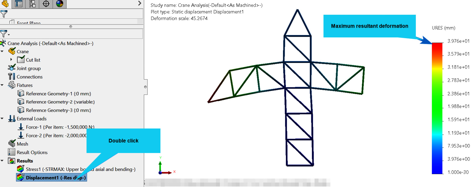
Figure 2.33 – The default display of the resultant displacement plot

The legend describing the displacement plot (on the far right of the screen) displays the range of the displacement from a very low number (in blue) to the maximum value (in red). It also displays the legend with the scientific number format. It is always better to present the result in a more readable format. Therefore, in the next set of steps, we will edit the display of the maximum resultant displacement value by following the steps given next:

1. Right-click on Displacement1 (-Res Disp-) and then choose Edit Definition.
2. From the Displacement plot property manager that appears, navigate to the Chart Options tab.
3. Under Display Options, tick inside Show max annotation.
4. Under Position/Format, change from scientific to floating.
5. Click OK.

Figure 2.34 indicates that with a combined load of 3500 kN applied to the crane, the maximum deformation experienced by one of the joints is 39.764 mm.

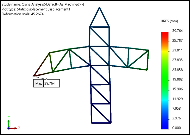
Figure 2.34 – The deformed shape of the crane and its maximum resultant displacement

Note that since a truss element has three translational displacement degrees of freedom at its node, the resultant displacement refers to the vectorial resultant displacement.

Obtaining the factor of safety

The factor of safety (FOS) is one of those results that are not automatically displayed but need to be retrieved during the post-processing of the results. From knowledge of the mechanics of materials, we know that the calculation of the factor of safety is based on certain failure criteria. SOLIDWORKS Simulation offers four failure criteria that we shall explore further in Chapter 5, Analyses of Axisymmetric Bodies. Nonetheless, irrespective of the criterion used in calculating the FOS, the rule of thumb is that the component we are analyzing has failed if the FOS is less than 1. But if the FOS is greater than 1, then the component is considered safe to support the applied load without failing (all things being equal). To retrieve the FOS, in the simulation study tree, do the following:

1. Right-click on the Results folder.
2. Select Define Factor Of Safety Plot (Figure 2.35 (a)).
3. The Factor of Safety property manager appears. Leave all options as they are as indicated in Figure 2.35 (b). Notice that the failure criterion is set to Automatic. Also take note of the navigating arrow that unveils further options.
4. Click OK.

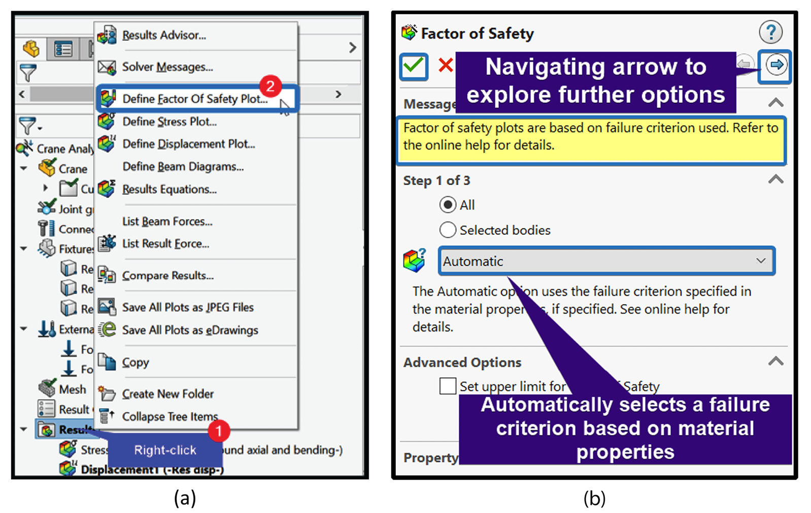
Figure 2.35 – (a) Retrieving the factor of safety; (b) the distribution of the factor of safety in the graphics window

Figure 2.36 reveals the distribution of the FOS for the crane upon the application of the load.

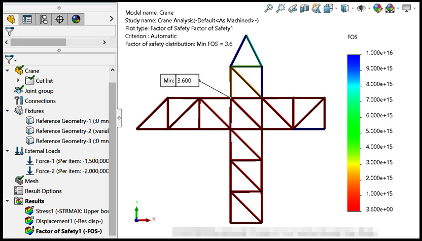
Figure 2.36 – Distribution of FOS over the crane

The figure indicates that the minimum FOS within the members of the crane is around 3.6, which means all is well with the crane. Note that by going with the Automatic option in step 3, SOLIDWORKS will use the failure criterion specified in the material property database, which is the Max Von-Mises failure criterion (see Figure 2.23).

Obtaining the axial force/stress for member IH

The last set of results we will look at is the axial forces and stresses. To retrieve either of these results, in the simulation study tree, do the following:

1. Right-click on the Results folder.
2. Select List Beam Forces (Figure 2.37 (a)).
3. Leave the options as indicated in Figure 2.37 (b).
4. Click OK.

   Note

   To retrieve the axial stresses, change to Stresses in the box labeled 1 in Figure 2.37 (b).

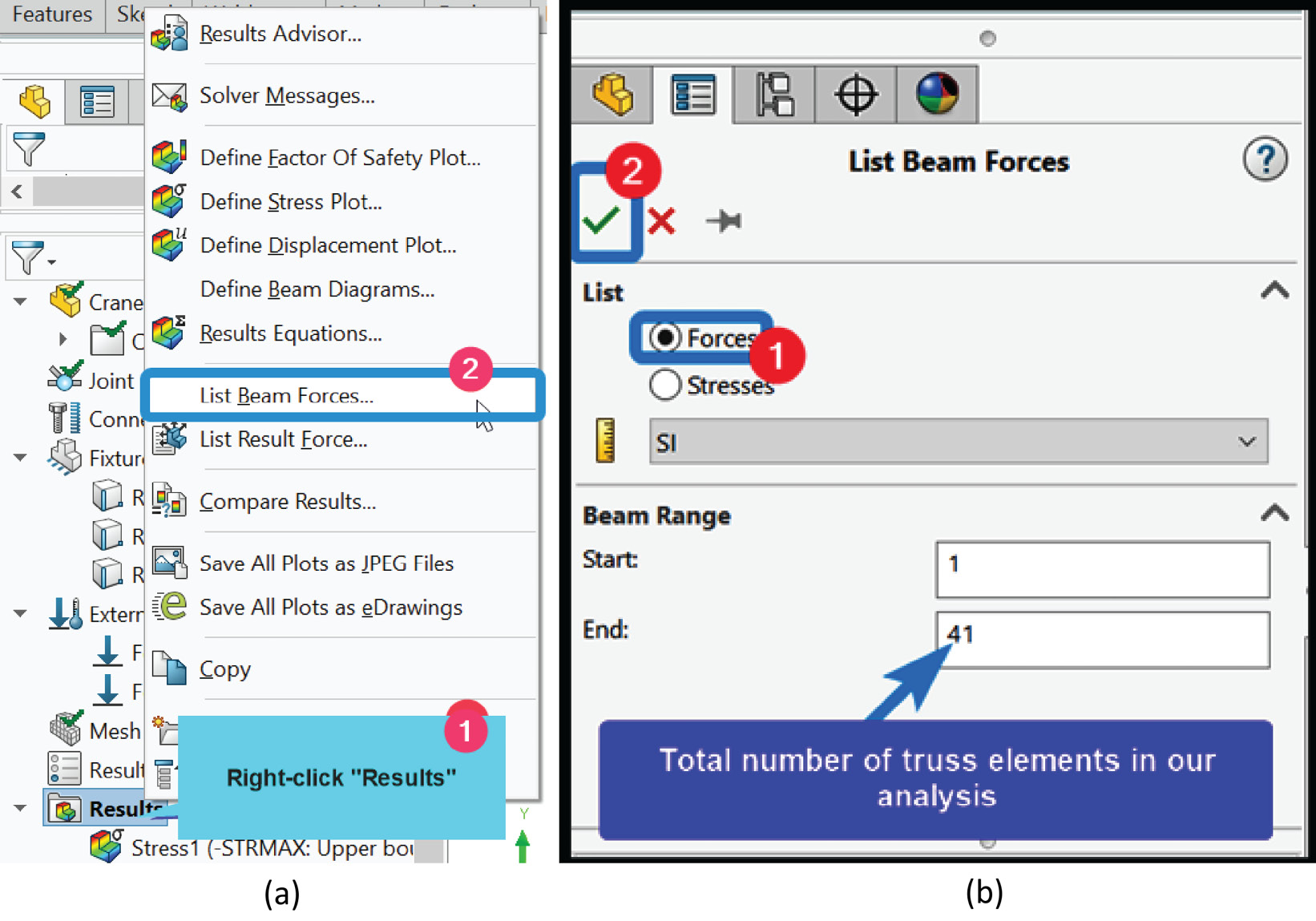
Figure 2.37 – (a) Retrieving the axial forces; (b) the beam forces property manager

Immediately after we complete steps 1-4, the List Forces window will appear in the graphics window as shown in Figure 2.38. You may use the arrow (marked 2) in Figure 2.38 to navigate through the values of the axial force developed in different members of the structure. You can also click on the name of a specific member and SOLIDWORKS will instantly highlight it in the graphics window.

For instance, Beam-19 (be aware that the name of this member will likely be different in your case) is the element that corresponds to member IH. It has been highlighted within the List Forces window for convenience. As you can see, this element experiences an internal axial force of approximately 727 kN. This value is within 3% of the answer (707 kN) obtained in [1]. Note that this is the only value computed in [1], simply because it is not trivial to carry out the manual calculations of the other values (displacements, FOS, forces, and stresses) without incurring substantial errors. Indeed, the small difference between the value from SOLIDWORKS and the cited reference may be attributed to possible rounding off errors.

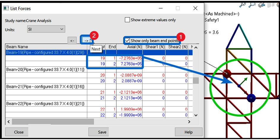
Figure 2.38 – The default display of axial forces

In many practical instances, you will want to list out all the forces/stresses for further examination. To do this, simply click on the column name Axial (N) (labeled 1) in Figure 2.39. This will give a compact display of the values of all 41 elements used in our analysis. From here, click on the Save button at the bottom of the List Forces window (labeled 3) to save all the data to an Excel file, then click Close to close the window. Afterwards, you can explore the data in Microsoft Excel.

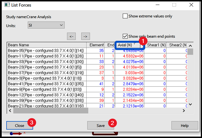
Figure 2.39 – Preparing the data for further post-processing

You will notice that beyond the axial forces, the List Forces window has other columns, such as Shear1, Shear2, and so on. At the moment, they all are zeros because we are employing the truss element option. For analyses that require the use of beam elements such as frames, they will not be zero.

Other things to know about the truss element

We have used the truss element in this chapter to study the computer analysis of a crane idealized as a 2D planar truss. However, the truss element and the procedure outlined in this chapter are also perfectly suitable to study straight bars and 3D space trusses. For conciseness, the deployment of the truss element to investigate the structural performance of components made of simple bars is demonstrated in the computer file of the first exercise question at the end of this chapter.

Summary

This chapter has covered some basic concepts in the use of SOLIDWORKS Simulation for the static analysis of trusses. We have explored how to create the skeletal lines describing a truss structure and the conversion of these line sketches into structural members with volume elements using the weldments tool. Overall, the following ideas have been addressed:

• How to activate weldment tool for structural analysis
• How to edit the cross-section of in-built profiles for specific needs
• How to change structural beam elements to truss elements
• Applying loads and fixtures on specific joints of a truss structure
• Modifying the displacement plot and obtaining the factor of safety

In the next chapter, Chapter 3, Analyses of Beams and Frames, we will study the use of beam elements for the analysis of transversely loaded components and study the usefulness of these elements for more complex analyses.

Questions

1. Figure 2.40 shows two straight segments of a machine loaded as shown. The segments are made of alloy steel and have a cross-sectional profile with an external and internal diameter of 40 mm and 20 mm, respectively. Treat the segments as two connected bars, then use SOLIDWORKS Simulation to do the following:

   a. Determine the displacement of end C.

   b. Evaluate the axial stresses developed in the components upon loading.

   

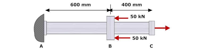
   Figure 2.40

2. Figure 2.41 shows a 2D plane truss representing a load-supporting mechanism. Components CB and AB are made of ASTM A-36 steel tubes with the same cross-section (external and internal diameters of 50 mm and 30 mm , respectively). Use SOLIDWORKS Simulation to do the following:

   a. Determine the resultant displacement of joint B

   b. Determine the minimum factor of safety of the assembly

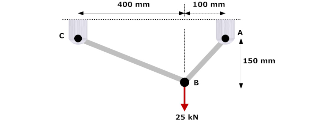
Figure 2.41

Further reading

[1] Structural and stress analysis, T. H. G. Megson, 4th, Ed, Butterworth-Heinemann, 2019.