Chapter 4: Analyses of Torsionally Loaded Components

One interesting aspect of SOLIDWORKS simulation is that it facilitates the analysis of components with virtually all types of loads that we meet in practical circumstances. In Chapter 2, Analyses of Bars and Trusses, we studied truss structures, which are made of bars (members under the effect of axial loads). In Chapter 3, Analyses of Beams and Frames, we shifted our attention to beams and frames (focusing only on transverse loads applied perpendicular to the axis of these structures).

One fairly basic type of load we have not studied is the torsional load. The goal of this chapter is to cover structures with this type of load. Along the way, we will demonstrate a suite of new features within the SOLIDWORKS simulation environment. Primarily, we will walk through the following topics:

• Overview of torsionally loaded members
• Some strategies for dealing with multi-segment torsionally loaded components in a SOLIDWORKS simulation
• Getting started with an analysis of torsionally loaded members in a SOLIDWORKS simulation

Technical requirements

You will need to have access to the SOLIDWORKS software with a SOLIDWORKS simulation license. You will also need to have acquired some knowledge of stress, strain, and material behavior.

You can find the sample files of the models required for this chapter here: https://github.com/PacktPublishing/Practical-Finite-Element-Simulations-with-SOLIDWORKS-2022/tree/main/Chapter04

Overview of torsionally loaded members

This section provides basic background information regarding torsionally loaded members. It gives the objectives of simulating these structures and their applications.

Components that are torsionally loaded may come under various categories, for instance:

• Shafts (cylindrical bars) that are under the action of twisting moments, or non-cylindrical one-dimensional structures under the action of pure twisting moments
• Beams that are loaded with shear loads for which the points of application do not coincide with the shear center of the beam section
• Grids that involve a collection of beams arranged as a framework supporting both transverse and torsional loads
• Space frames with members under the effect of torsional loads combined with other types of loads (such as axial plus bending loads)

All four categories listed above have notable applications. Nevertheless, in the rest of this chapter, we will restrict ourselves to the first category. Reasons for this include brevity and the fact that their wide applications can be easily spotted in our surroundings. Besides, they represent a straightforward way to demonstrate the concept of twisting deformation and of shear stress. Moreover, this category also represents the workhorse of rotating machinery – from the shaft of a car experiencing a torque from the engine, or a construction auger, to propeller shafts for wind and hydroelectric power generation [1] and [2] (see the Further reading section). Furthermore, when we use simple machines such as a lug wrench or screwdriver, torsional loading is at play.

Figure 4.1 shows some examples of machines that work based on the behavior of torsionally loaded components experiencing twisting moments.

Principally, when a shaft is torsionally loaded, shear stresses develop within it. Furthermore, the shaft experiences a twisting deformation (called the angle of twist) about its longitudinal axis. Consequently, a primary aim of the static analyses of torsionally loaded components relates to finding these quantities (that is, shear stresses and angle of twist) to help in design tasks.

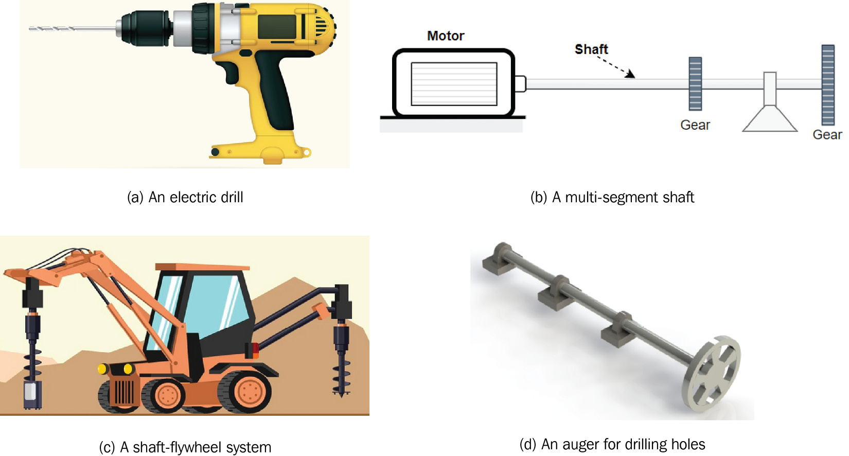
Figure 4.1 – Some applications of torsionally loaded components in practice

The four examples shown in Figure 4.1 are indicative of various types of torsionally loaded shafts. But there are some subtle differences in the way we can analyze them. For instance, the shaft facilitating the transmission of the load from the motor (see Figure 4.1b) and the one supporting the flywheel (in Figure 4.1c) exemplify the kind of components suitable for the approach we will demonstrate in this chapter. The other two examples are best analyzed using the approach we will present in Chapter 6, Analysis of Components with Solid Elements.

Having described some features of torsionally loaded shafts, we can now expand upon the strategy for their computer analysis.

Strategies for the analysis of uniform shafts

This section describes the structural details and the modeling strategy for the analysis of shafts using the SOLIDWORKS simulation environment.

Structural details

The technical details presented for the analysis of beams/frames in Chapter 3, Analyses of Beams and Frames, are also applicable to the analysis of simple shafts. This means you will need to know the following technical details ahead of the analysis:

• Dimensions:
  • Details of the cross-section
  • Geometric length
• Material properties
• External loads applied to the shaft
• The support provided to the shaft to prevent rigid body motion

Modeling strategies

The strategy to be adopted for creating the geometric model of a shaft to be analyzed will often depend on the complexity of the structural details. Assuming we restrict ourselves to long straight shafts with simple and uniform cross-sections, then we may choose to adopt either of the following approaches:

• Model the shaft using the method of extruded cross-sections
• Model the shaft based on the application of the weldments tool

When a shaft is created using either of the preceding approaches, then the simulation of its behavior can be conducted using the beam element within the SOLIDWORKS simulation engine.

Now, we have already dealt with the use of the weldments tool in Chapters 2, Analyses of Bars and Trusses, and Chapter 3, Analyses of Beams and Frames. Therefore, in this chapter, we will adopt the second approach so that it becomes obvious that we can, in fact, use the beam element without going through the use of the weldment tool.

But irrespective of which modeling approach you adopt, be mindful of the idea of critical positions we mentioned in Chapter 3, Analyses of Beams and Frames. With shafts, as with beams, the extruded sections should (in most cases) be created based on the knowledge of critical positions. To illustrate the concept of critical positions, Figure 4.2 shows a multi-segment shaft with the critical positions labeled from A – G. As you will observe, the following points are treated as critical positions:

• The beginning and end of the members in a multi-segment shaft
• A point where a concentrated torque is applied
• The beginning of a distributed torque
• The end of a distributed torque
• A point where there is a change of cross-section

Figure 4.2 – An illustration of the critical positions (labeled A - G) in a multi-segment shaft

• A point where there is a change of material properties
• All points of support
• All points of connections

This list is by no means exhaustive, but it should give you an idea of when to use this concept. Note that it is not always necessary to treat these points as critical. For instance, if you are not interested in reading the stress or the deformation of segment BD or at points B and D (Figure 4.2), then you don't have to treat them as critical positions.

Characteristics of the beam element in a SOLIDWORKS simulation library

We have already used the beam element in Chapter 3, Analyses of Beams and Frames. Hence, you may be prompted to ask: How is it possible that we can use a beam element to analyze torsionally loaded components? Well, the answer lies in the fact that the beam element provided in the SOLIDWORKS simulation library is a three-dimensional element that can support three translational displacements along the x, y, and z axes, and three rotational displacements about these three axes. The rotational displacement about the longitudinal axes is what corresponds to the twisting deformation in the analysis of torsionally loaded components such as shafts. Furthermore, shear stress from torsional loads is one of the six stress components that can be extracted when the beam element is used.

With the information provided in this section, it is time to walk through a case study to demonstrate the analysis of a component with torsional loads.

Getting started with analyses of torsionally loaded members

The case study in this section illustrates the use of the beam element without relying on the weldment tool for analyses of components with torsional loads. Further, it demonstrates how to define a custom material within the SOLIDWORKS simulation environment and shows the retrieval of shear stress and angle of twist.

Time for action – Conducting a static analysis of a multi-material, stepped shaft with torsional loads

Problem statement

A compound shaft is formed by bonding an aluminum rod, AB, to the brass rod, BD. The shaft is loaded with torque at positions B and A, as shown in Figure 4.3a, while the length of its segment and a sectioned view of the shaft is revealed in Figure 4.3b. The DC portion of the brass segment is hollow and has an inner diameter of 40 mm. The D end of the shaft is connected to a wall, which is acting as fixed support. We are interested in simulating the loading of the shaft and consequently obtaining the following:

• The angle of twist of end A
• The maximum shear stress in the brass segment

This problem is inspired by exercise 3.38 in the book by Beer, et al. [2]. In the solution, the authors obtained a value of 6.02 degrees for the angle of twist at position A. Can we use a SOLIDWORKS simulation to verify this answer?

Let's dig in.

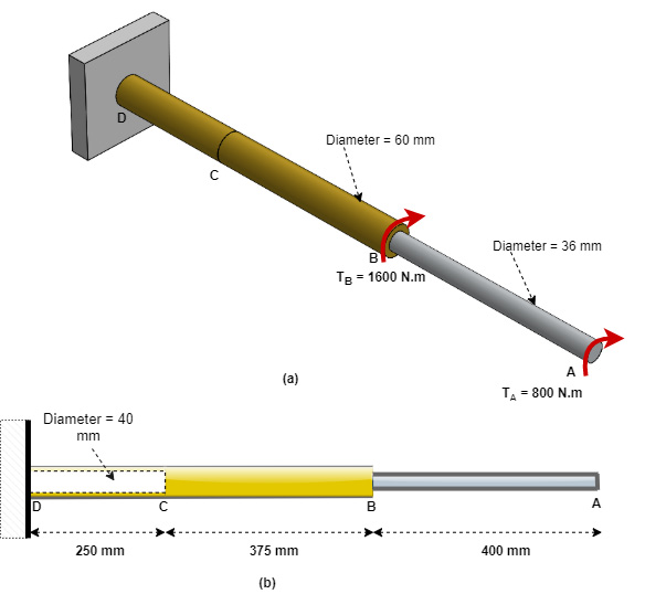
Figure 4.3 – (a) Isometric view of a shaft made of brass and aluminum with torsional loads; (b) a schematic of the shaft with the length of the segments and diameter of the hollow segment

In what follows, we will use the SOLIDWORKS simulation to analyze the problem and address the questions posed. Let's start with the creation of the model, as has been the practice from the previous chapters.

Part A – Creating a 3D model of the shaft using the extrusion of cross-sections

We will create a 3D model of the shaft segments on the right plane. However, note that the model can also be created on the front plane. Before we start the creation of the 3D model of the shaft, notice that points D, C, B, and A are critical points (according to what was mentioned in the earlier sub-section – Modeling strategies). Specifically, points D and A are the extreme ends of the shaft, while points C and B are treated as critical points because of the change of cross-section. Of course, we also note that points B and A are the positions of the applied torques. As a rule of thumb, any segment that falls between two critical points has to be created independently, as you will see next.

To begin, start up SOLIDWORKS (File  New  Part) and save the file as Shaft. Ensure the unit is set to the MMGS unit system.

Creating segment DC

We will start with the creation of segment DC (the hollow segment of the shaft):

1. Click on the Sketch tab.
2. Click on the Sketch tool.
3. Choose Right Plane, as shown in Figure 4.4:
   

   Figure 4.4 – Choosing Right Plane

4. Select the Circle sketching command and create two concentric circles and dimension them as shown in Figure 4.5.
5. Navigate to the Features tab, and then click on Extruded Boss/Base:
   

   Figure 4.5 – Instantiating the extruded command (units in mm)

   Step 5 brings up the Boss-Extrude property manager.

6. Within the Depth box (marked 1 in Figure 4.6), key in the value of 250 mm for the depth of the extrusion.
7. Click OK (the green ) to get the extruded model of segment DC, as shown in Figure 4.6:

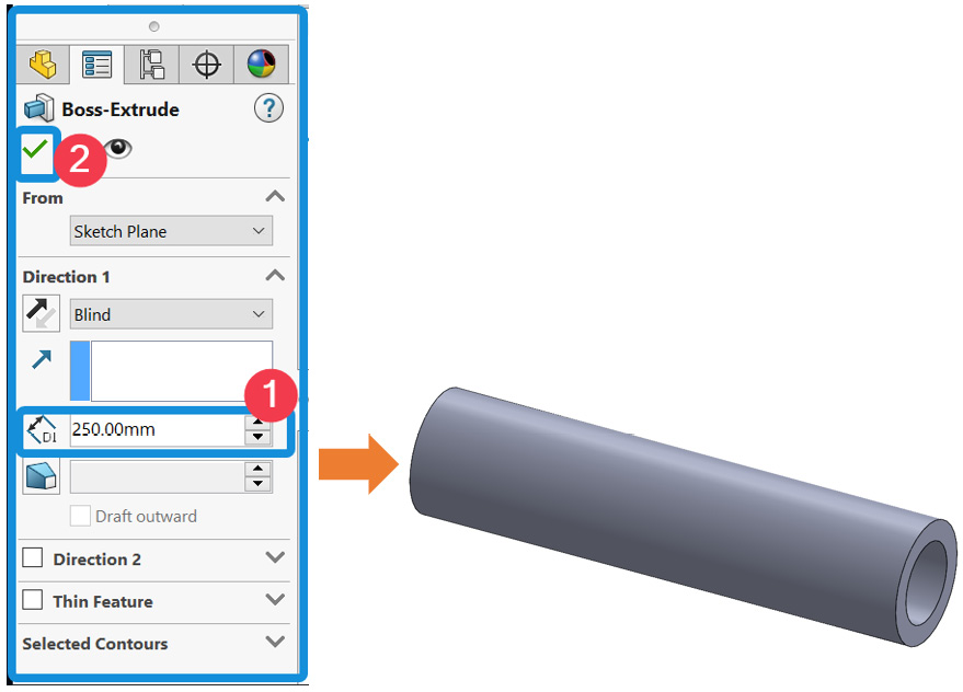
Figure 4.6 – An extruded segment of length 250 mm

We have now created the first segment, and we are set to create the second segment (CB) of the shaft in the next sub-section.

Creating segment CB

Segment CB is a solid segment with a diameter that is based on the outside diameter of segment DC. Therefore, the base sketch to be extruded for this segment will be overlaid on the right end of the completed segment DC. To this end, follow the steps listed next to create segment CB:

1. Click on the right end of segment DC (created in the preceding section). A context toolbar will appear shortly afterward, as shown in Figure 4.7.
2. Choose Normal to so that the face is oriented.
   

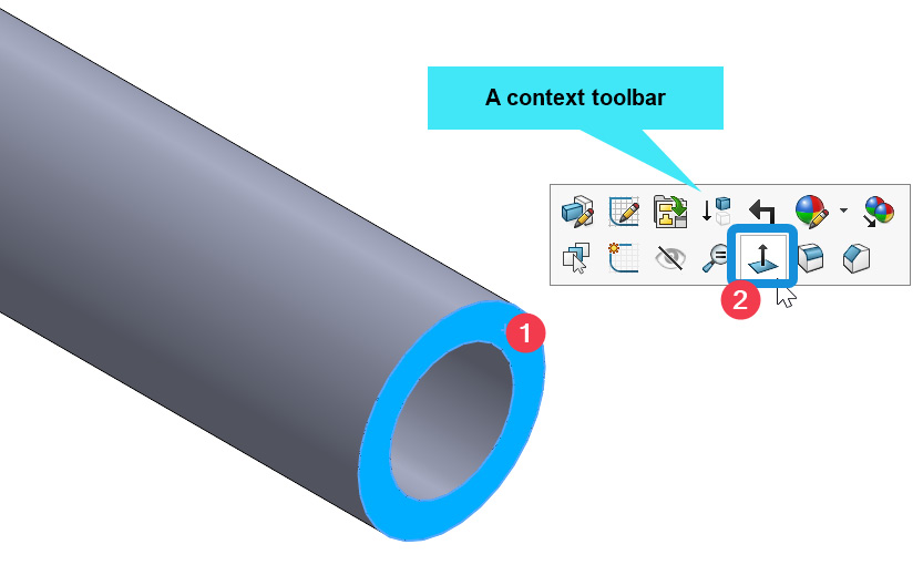
   Figure 4.7 – Selections to orient the right end of segment DC

3. After the face is oriented, click on the face again so that the context toolbar re-appears.
4. Then, select Sketch, as shown in Figure 4.8:
   

   Figure 4.8 – Preparing to sketch on the oriented face

5. Pick the Circle sketching command to create a 60 mm diameter circle.
   

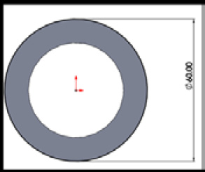
   Figure 4.9 – A sketched circle with a diameter of 60 mm

6. Navigate to the Features tab.
7. Click on Extruded Boss/Base (Figure 4.10):
   

   Figure 4.10 – Activating the extruding feature

   The completion of step 7 will activate the Boss-Extrude PropertyManager. Now we will work with the options highlighted in the next steps that follow.

8. Under the Depth box (marked 1 in Figure 4.11a), key in the value of 375 mm for the depth of the extrusion.
9. Untick Merge result (marked 2 in Figure 4.11a).

   Important Note

   Step 9 is very important. Ensure you untick Merge result before clicking OK.

10. Click OK (the green ).

Following completion of the preceding steps, you will get the extruded model of segment CB, as shown in Figure 4.11b:

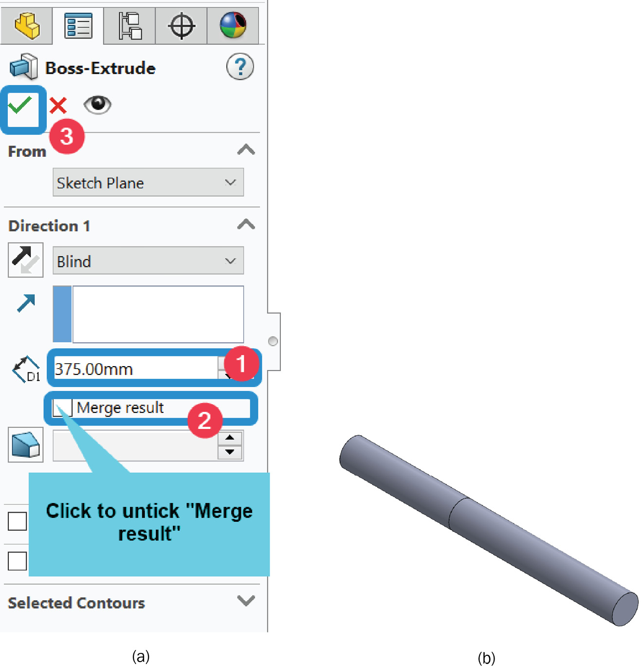
Figure 4.11 – Options for creating the second extruded segment (CB)

Note that step if Step 9 is omitted, SOLIDWORKS will merge the two segments and a joint will not be created between the two different cross-sections. The consequence of this is that you will not be able to apply a torque or easily read the angle of twist at the intersection between the hollow and solid brass segments.

With these two segments created (that is, DC and CB), we next move on to the creation of the last segment of the shaft in the next sub-section.

Creating segment BA

Segment BA is also a solid segment. As we did in the preceding sub-section, we will overlay the base sketch of this segment on the right end of the just-completed segment CB. The steps to create segment BA are similar to what was outlined for the creation of segment CB.

To this end, follow the steps given next:

1. Click on the right end of segment CB (created in the preceding section). A context toolbar will appear shortly afterward.
2. Choose Normal to so that the face is oriented.
3. After the face is oriented, click again on the face so that the context toolbar re-appears.
4. Select Sketch, as shown in Figure 4.12:
   

   Figure 4.12 – Preparation for sketching on the oriented face of segment CB

5. Pick the Circle sketching command to create a 36 mm diameter circle.
   

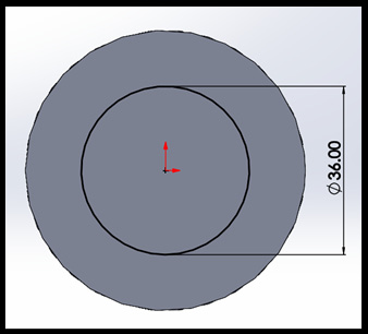
   Figure 4.13 – A sketched circle with a diameter of 36 mm

6. Navigate to the Features tab, and then click on Extruded Boss/Base.

   Again, this step depicts the Boss-Extrude property manager (see Figure 4.14).

7. In the Depth box, key in the value of 400 mm for the depth of the extrusion.
8. Untick the Merge result checkbox.
9. Click OK (the green ) to get the extruded model of segment BA:

Figure 4.14 – Options for creating the second extruded segment (CB)

The new status of the model of the shaft in the graphic window should look like Figure 4.15. Notice that the FeatureManager tree should contain three bodies, as indicated:

Figure 4.15 – A complete extruded model of the shaft with the distinct segments

At this point, we have completed the creation of the model of the shaft. In the next sub-section, we will launch the simulation study.

Part B – Creating the simulation study

This section comprises three sub-sections. The first sub-section will see us going through the activation steps for the simulation study, after which we shift our focus to the conversion of the extruded solid bodies to the beam element. The final sub-section deals briefly with contact settings.

Let's start with the creation of the simulation study.

Activating the Simulation tab and creating a new study

To activate the simulation commands, follow the steps highlighted next:

1. Click on SOLIDWORKS Add-Ins.
2. Click on SOLIDWORKS Simulation to activate the Simulation tab (Figure 4.16):
   

   Figure 4.16 – Activating the Simulation tab

3. With the simulation tab active, click on New Study:
   

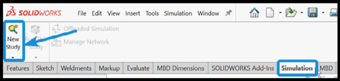
   Figure 4.17 – Creating a new study

   Now we will work with the options within the Study property manager (Figure 4.18).

4. Input a study name within the Name box, for example, Shaft analysis.
5. Keep the Static analysis option (selected by default).
6. Click OK (that is, the green checkmark).

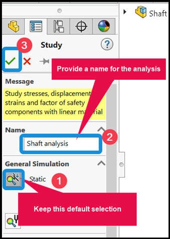
Figure 4.18 – Study names and options

With the completion of steps 1-6, the simulation study tree becomes active, as depicted in Figure 4.19:

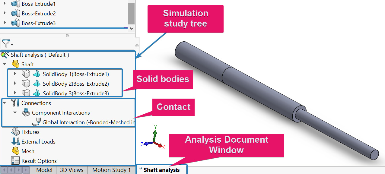
Figure 4.19 – Simulation property manager

Two details can be observed if you examine the simulation study manager (Figure 4.19):

• The first observation is that each extruded segment of the shaft has been converted into a solid body. Because we have three segments, there are three solid bodies (in other words, SolidBody1, SolidBody2, and SolidBody3). This differs from what happened when we used the weldment approach (in Chapter 2, Analyses of Bars and Trusses, and Chapter 3, Analyses of Beams and Frames), where the parts are automatically converted to beam elements after initiating the study.
• The second observation relates to the fact that SOLIDWORKS has defined a Global Interaction under the Connections property name. This global interaction describes the contact defined between each of the three segments. Each of these two observations is expanded upon in the next two sub-sections.

Let's start with the transformation of the extruded solid bodies.

Note – Change of Terminology in SOLIDWORKS 2021-2022

If you are using an earlier version of the SOLIDWORKS simulation, what you will see under the Connections property name is Component Contacts and Global Contact instead of Component Interactions and Global Interaction.

Converting the extruded solid bodies to beams

Since we wish to use the beam element, we will have to convert the solid bodies created under the simulation study tree into beams by following the next two steps:

1. Select all three bodies as shown in Figure 4.20 (for example, select Solidbody1, press and hold down the control key, and then select the other two bodies).
2. Right-click within the region containing the selected bodies and then click on Treat selected bodies as beams.

   Note

   If you forget to convert the extruded solid bodies into beams, then SOLIDWORKS will automatically employ solid elements for the simulation. Practically, there is no harm in using solid elements to analyze the shaft. However, if that happens, you will not be able to easily extract the angle of twist for the shaft. Why? As you will see in Chapter 6, Analysis of Components with Solid Elements, solid elements do not support rotational degrees of freedom.

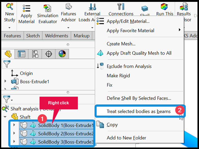
Figure 4.20 – Converting solid bodies into beams

After completing steps 1-2, there will be a change in the symbol attached to each of the three bodies from to (which symbolizes beams). Along with this change, joints will be created at the critical positions of the shafts, as shown in Figure 4.21:

Figure 4.21 – Creation of beams and joints

Meanwhile, in Figure 4.21, you will notice the warning sign attached to the first body. As a result of this warning, an Error notification appears beside the analysis name. The beam warning arises from the fact that the length to diameter ratio for the first segment is less than 10, which is true. However, the consequence of violating this warning is not fatal for this analysis and can be safely ignored (as will be confirmed by our final results).

In many instances, when an error notification is attached to our analysis name, it is a good idea to find out the reason. This can be done as illustrated in Figure 4.22. Usually, after clicking What's wrong?, a diagnostic message about the cause of this error will appear.

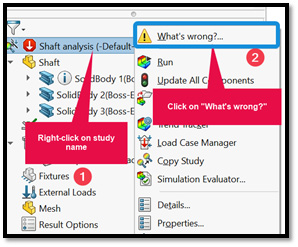
Figure 4.22 – Finding out more about an error/warning

Information

Beam Warning: Hovering over the beam with the warning sign (Figure 4.21) will give information that this segment is too short to be considered a beam. This is because the classical beam theory demands that the slenderness ratio (that is, the ratio of the length/characteristics dimension, for example, L/width or L/height or L/diameter) of any segment to be considered a beam should be greater than 10.

So far, you have covered the steps for the transformation of extruded bodies into beams. You have also taken a short peek into the evaluation of an error warning within the simulation study.

Let's wrap up this sub-section by checking on the contact settings.

Scrutinizing the interaction settings

You will recall that during the modeling phase in section A, each segment of the shaft segment was extruded without being merged with the preceding one. This is an important strategy for dealing with multi-segment components. However, in realistic engineering scenarios, the segments are to be perfectly bonded. Based on this logic, a SOLIDWORKS simulation automatically defines interactions between the unmerged extruded bodies. The question that arises from this is: What type of interaction is defined between the bodies?

To answer the above question, this sub-section briefly discusses interaction settings generated by a SOLIDWORKS simulation between the three segments of the shaft.

To this end, perform the following steps to scrutinize the interaction settings:

1. Expand each of the beams to expose the contact setting between each segment, as shown in Figure 4.23:
   

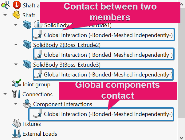
   Figure 4.23 – Appearance of Component interaction settings

2. Next, right-click on one of the exposed Global Interaction option and choose Edit Definitions. This will lead to the appearance of the Component Interaction property manager. Keep the options as shown in Figure 4.24:

Figure 4.24 – Component interaction property manager

You will notice that we have a Global Interaction defined under the Connections property name. The Global Interaction defines the contact condition that applies to all components in multi-body parts or assemblies. It is this definition that is propagated under the shaft segments as shown in Figure 4.23. Principally, interaction settings define the relationship between entities that have initial contact or have the possibility to touch each other during loading. As you will notice in Figure 4.24, three types of interactions are listed under Interaction Type:

• Bonded
• Contact
• Free

  Note

  If you are using an earlier version of the SOLIDWORKS simulation, what you will see within the Component Interaction property manager under the Interaction Type option are: No Penetration (this is now known as Contact); Bonded; and Allow Penetration (this is now known as Free).

Now, as seen in Figure 4.24, the default selections are Bonded with the option to Enforce common nodes between touching boundaries. So, what does this mean? In effect, this choice indicates that the components affected by this choice will act as if they are welded during simulation. As a result, the Bonded interaction type is perfect for this simulation since we will want the segments of the shaft to be perfectly in touch with each other to account for the artificial joints we introduced at the critical positions.

Meanwhile, the simulation environment may show other categories of interaction (not seen in Figure 4.24) depending on the types of bodies that are in interacting with one another. For this reason, in Chapter 7, Analyses of Components with Mixed Elements, we will re-visit the options for interactions when we combine different higher-order elements.

At this point, we have completed the initiation of the simulation study. We have also learned about the conversion of extruded bodies into beams without making use of the weldments tool. Furthermore, we have taken a cursory look at interaction settings.

Next, we will learn about how to create a custom material and apply material properties to different segments of the shaft.

Part C – Creating custom material and specifying material properties

In Chapter 2, Analyses of Bars and Trusses, and Chapter 3, Analyses of Beams and Frames, we have applied a single type of material to the components that we analyzed. Moreover, in those chapters, we accepted the values of the material properties contained in the SOLIDWORKS materials database.

In this section, you will learn how to create a custom material from a base material within the library.

You may be wondering why we need to create a custom material. Recall that from the problem statement, segments DC and CB are made of brass (G = 39 GPa), while segment BA is made of aluminum alloy (G = 27 GPa). There is an aluminum alloy in SOLIDWORKS materials database with the exact shear modulus (that is, G = 27 GPa) as we have in the problem statement. Hence, it is a straightforward matter to apply the property for segment BA. However, as will be shown next, the grade of brass within the library has a shear modulus, G = 37 GPa, which is slightly lower than what was specified in the problem statement. Although the difference is small, we will use this opportunity to showcase how to create a custom material.

Let's get going.

Creating and applying a custom material property (custom brass)

There are a few ways to create custom materials in SOLIDWORKS. You may create a new custom material from scratch if it is not available within the materials database. But you can also work from a material that is already within the database, in which case we simply modify the values of the properties to suit our needs. The method we will demonstrate in this section adopts the latter approach.

To this end, perform the following actions under the simulation study tree:

1. Select segments DC and CB (representing the brass segments).
2. Right-click within the colored area of the selected items.
3. Click Apply/Edit Material... (Figure 4.25):

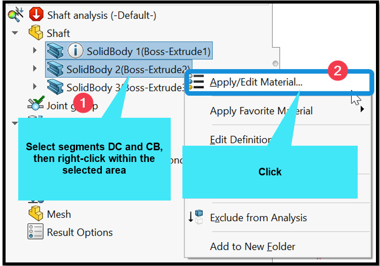
Figure 4.25 – Activating the material database

As soon as you complete steps 1-3, the material database appears (which you saw in Chapter 2, Analyses of Bars and Trusses, and Chapter 3, Analyses of Beams and Frames).

We are interested in brass, which is a copper alloy. Therefore, to create a custom brass from this in-built brass material, follow the steps given next.

While the material database is still on, perform the following steps:

1. Expand the Copper Alloys folder to locate Brass.
2. Right-click on Brass and choose Copy (Figure 4.26):
   

   Figure 4.26 – Copying the properties of the built-in brass

3. Scroll down to the material folder named Custom Materials, right-click, and choose New Category (Figure 4.27):
   

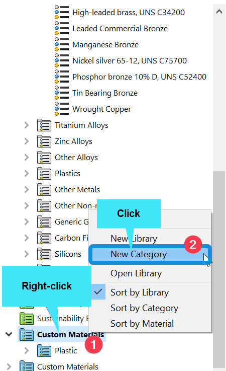
   Figure 4.27 – Navigating to the custom material section

   Under the Custom Materials folder, a new material folder will be created with a default name New Category.

4. Change the name to MyBrass (Figure 4.28).
5. Right-click on the newly created MyBrass folder and select Paste from the context menu that appears (Figure 4.28):

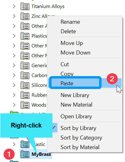
Figure 4.28 – Selection of options to create a custom brass from the base brass material

At this point, we have copied and pasted all the properties of the in-built brass. We are now ready to update the property of the brass to suit our needs. Note that after the preceding step (in other words, step 5 above), a material named Brass is created under the MyBrass folder (see Figure 4.29). To avoid confusion, perform the following steps:

1. Right-click on the new Brass material and rename it Brass-39 as depicted in Figure 4.29.
2. Change the shear modulus to 3.9e+10, as shown in Figure 4.29.
3. Keep the failure criterion as Max von Mises Stress.
4. Click Save.
5. Click Apply and Close (in that order).

Figure 4.29 – The material database and the options for creating a custom brass

Before we transition to the next action, take note of the four failure theories that SOLIDWORKS supports for linear elastic isotropic materials. The names of these theories, as highlighted in Figure 4.29, are as follows:

• Max von Mises Stress
• Max Shear Stress (Tresca)
• Mohr-Coulomb Stress
• Max Normal Stress

Each of these criteria specifies the condition under which an isotropic material fails. The first two apply to ductile materials (such as steel). In contrast, the last two are used for the failure prediction of brittle materials. SOLIDWORKS will, by default, use the von Mises failure theory for analyses of ductile materials. The fundamental idea of this theory dictates that in a component made of ductile material, if the maximum von Mises stress exceeds the yield strength of the material from which the component is made, then yielding of the component will happen. For further details about the aforementioned theories, you may refer to the books by Beer, et al. [2] or Collins, et al. [3], among others.

In any case, after completing steps 1-5, a tick mark will appear on segments DC and CB. But there are three segments within the shaft, and we need to specify the material for the last segment. This is what we do in the next sub-section.

Adding a material property (aluminum alloy)

Here, we will apply the material details to segment BA of the shaft. This segment is made of aluminum alloy. To apply the aluminum material property, follow the steps given next:

1. Right-click on segment BA and choose Apply/Edit Material.
2. Expand the Aluminium Alloys folder.
3. Click on 1060 Alloy.
4. Click Apply and Close.

After closing the material database window, a green tick mark () will appear on the part's name.

At this point, we have completed the specification of the material properties for all segments of the shaft. Next, we will walk through the application of fixtures and torques.

Part D – Applying torque and fixtures

This sub-section focuses on how to set up the application of the torques (or twisting moments) at joints B and A of the shaft. We will also carry out the application of fixtures at joint D.

Let's begin with the application of fixtures.

Applying a fixture at joint D

We only have a single point of support for this problem located at joint D. To apply the fixture to this joint, follow the steps given next.

Under the simulation study tree, perform the following actions:

1. Right-click on Fixtures, and then pick Fixed Geometry from the context menu that appears.
2. Within the Fixture property manager that appears, select Fixed Geometry (Figure 4.30).
3. Navigate to the graphics window and pick joint D.
4. Click OK.

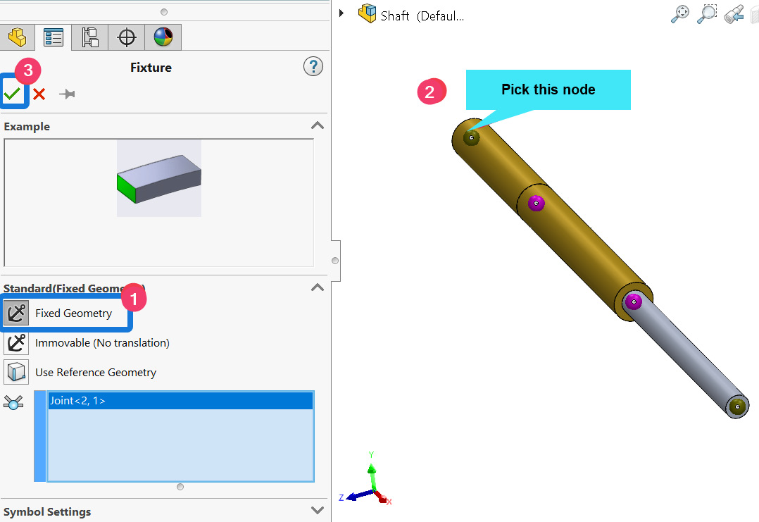
Figure 4.30 – Selecting the fixture for joint D

At the end of steps 1-4, the arrow symbolizing the fixed fixture will appear at joint D. This fixture restricts joint D so that all six degrees of freedom are zero.

With the fixture application completed, we now shift our attention to the application of the two twisting moments representing the payload torques.

Applying torque at joints B and A

In this sub-section, the torque we wish to apply is a type of moment that leads to the twisting of the longitudinal axis of the shaft.

Let's follow the steps given next to apply the torques at joints B and A.

Under the simulation study tree, perform the following actions:

1. Right-click on External Loads and select Torque (as shown in Figure 4.31):
   

   Figure 4.31 – Initiating the application of torque

   Now we will work with the options within the Force/Torque property manager that appears.

2. Under Selection, click on the joint symbol (labeled 1 in Figure 4.32).
3. Navigate to the graphic window to click on joint B.
4. Under the reference box direction (labeled 3 in Figure 4.32), choose the Front Plane.
5. Under Moment, activate the Along Plane Dir 1 box and input 1600 (ensure that the unit system remains an SI unit).
6. Click OK.

Figure 4.32 – Selections for the application of a twisting moment at joint B

Once steps 1-6 have been completed, a twisting moment will be applied to joint B.

Next, we need to apply another twisting moment to joint A. The steps are similar to what we have just done for joint B. For brevity's sake, Figure 4.33 captured the options to be made within the Force/Torque window:

Figure 4.33 – Selections for the application of a twisting moment at joint A

Following the application of twisting moments at joints B and A, the simulation study tree and the model in the graphics window will likely appear as shown in Figure 4.34.

You will notice that the arrow representing the two torques at these joints does not appear in the graphics window (as confirmed in Figure 4.34). This is because the torques are directed along the length of the shaft and they have been overshadowed by the third component.

Figure 4.34 – Appearance of the simulation study tree and the model

To see that we have truly applied the torques, we will reveal the features symbolizing them by following the steps given next:

1. Navigate to FeatureManager.
2. Right-click on Boss Extrude 3 (indicated by 1 in Figure 4.35a) and then select Hide from the context menu as shown in Figure 4.35a, the symbols representing the torques will appear as shown in Figure 4.35b.
3. Once you have seen the symbols, you may unhide the segment before running the analysis.

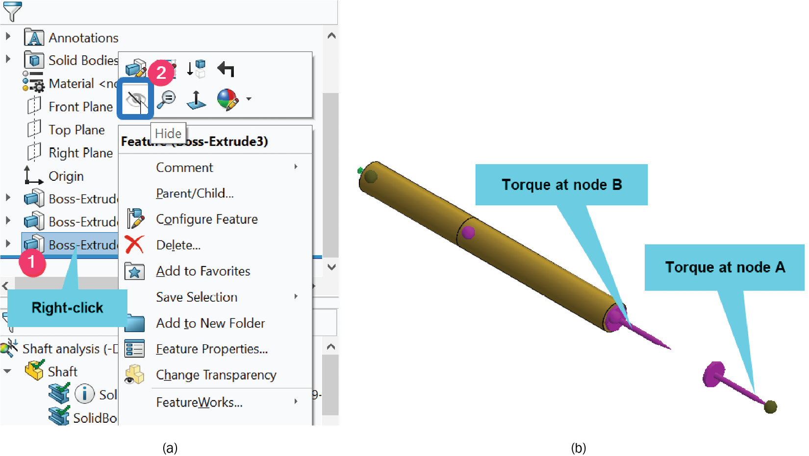
Figure 4.35 – (a) Options to hide segment BA; (b) exposing the torque symbol at joints B and A

This now concludes the application of torque on the joints of the shaft. We are getting close to completing the pre-processing tasks for the simulation.

So far, we have learned how to convert extruded entities into beams without using the weldments tool. In addition, we have covered how to create a custom material and showed how to modify the values of specific material properties. Besides, we have briefly examined contact settings and we have explored the application of torques. Now, we can move to the meshing task and running of the analysis, which is what happens in the next sub-section.

Mesh and Run

We have already examined the options to mesh and run our analysis in Chapter 2, Analyses of Bars and Trusses, and Chapter 3, Analyses of Beams and Frames. As explained in those chapters, any time we employ either the truss or beam element, a straightforward meshing command is Mesh and Run. Therefore, we will employ this same command here.

To that end, follow the steps given next:

1. Right-click on Mesh within the simulation study tree.
2. Select Mesh and Run.

After completing these two steps, the study tree will be updated with default results (Stress 1 and Displacement1), and the graphic window will display the deformed shape that corresponds to Stress1. However, these two results are not our focus.

In the next section, we will retrieve the results that we want.

Part E – Post-processing of results

Now that we have completed the steps in the previous sections, we will now attempt to address the following questions:

1. What is the angle of twist generated at joint A due to the combined effects of the two payload torques?
2. What is the maximum shear stress that developed within the shaft?

Let's begin with the retrieval of the angle of twist.

Obtaining the angle of twist at joint A

As with other types of loads, when a component is torsionally loaded with a torque (also known as a twisting moment), it experiences deformation, strain, and stress. And because a twisting moment creates a rotation of the material points on the cross-section of a loaded component, one of the notable deformations that arise from it is the angle of twist. An angle of twist is simply a rotational displacement of one end of a loaded component with respect to another. It is often quantified with respect to the axis through which the twisting moment acts.

To obtain the angle of twist experienced by the shaft, we follow these steps:

1. Right-click on Results and then select Define Displacement Plot.

   Now we will work with the options within the Displacement plot property manager (summarized in Figure 4.36) that appears.

2. On the Definition tab, navigate to Display.
3. Select RX: Rotation in X Direction and select the other options highlighted in Figure 4.36a.
4. Move to the Chart Options tab, under the Display options, and check the Show max annotation box.
5. Still within the Chart Options tab, under Position/Format, change the number format to floating, as depicted in Figure 4.36b.
6. Click OK.

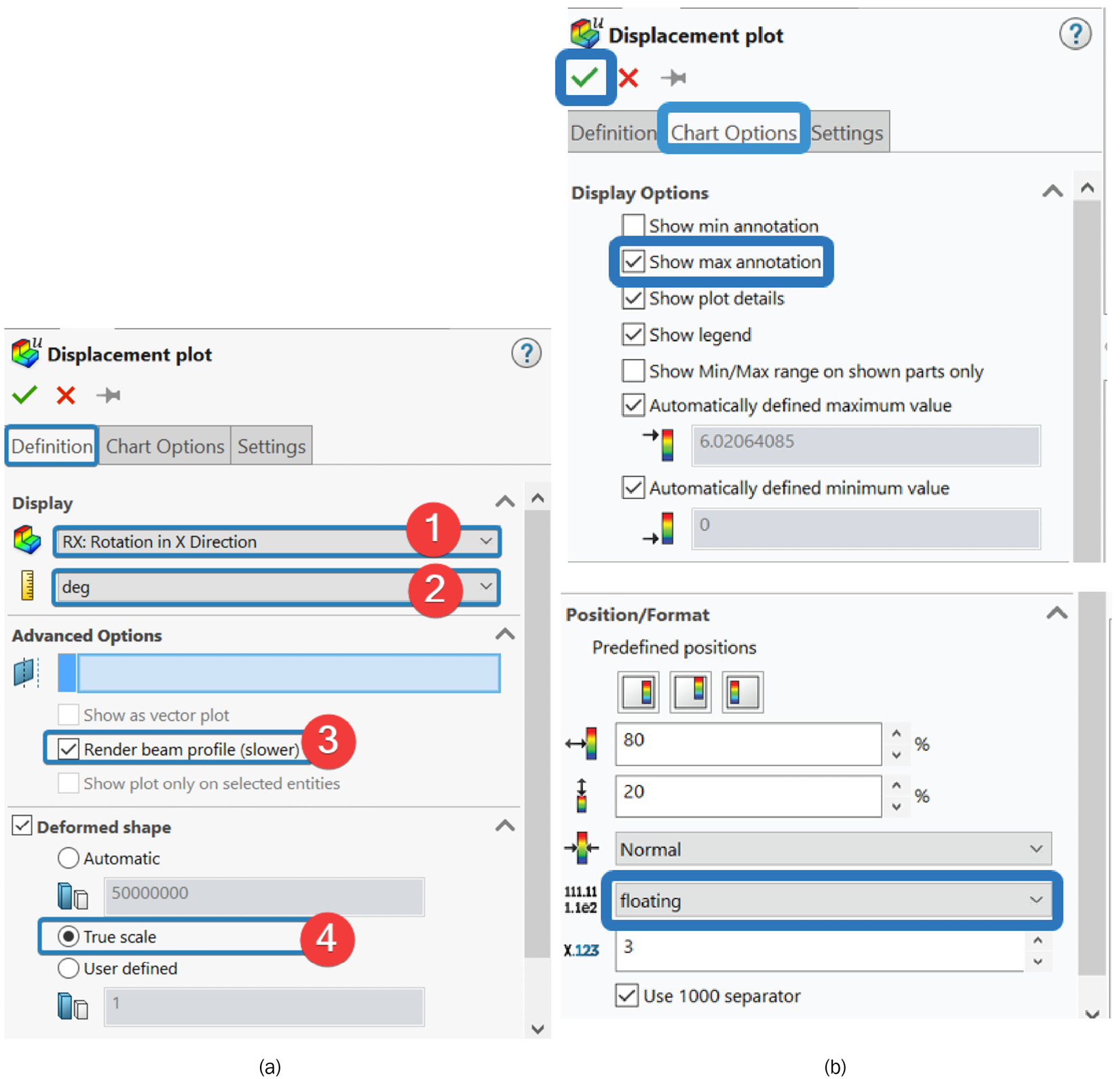
Figure 4.36 – Specifying options for the displacement plot

Figure 4.37 depicts the angle of twist (or the rotational displacement about the x axis) of joint A. This figure indicates that joint A experiences a rotational displacement of 6.02 degrees with respect to the fixed end (joint D). Furthermore, as a confirmation of the accuracy of this simulation, it is important to observe that the value of the angle of twist that we have obtained matches exactly the value reported in [2].

Figure 4.37 – The display of the rotational angle of twist

In Figure 4.37, notice that segment DC is bluish. This is because joint D, which is the end of the shaft, is fixed (that is, not allowed to rotate or move) when the torques are applied at joints B and A. Hence, the angle of twist at joint D is 0. The angle twist can be seen to increase from joint D (blue color) to joint A (red color). It is worth reiterating here that the main benefit of identifying the critical positions in our components during modeling is that we can obtain the deformation data at those positions during post-processing. So, go ahead and check the angle of twists at joints B and C.

Now, beyond the deformation data, it is always a good idea to check the stress experienced by the component. Therefore, we will set up the option for the evaluation of the shear stress in the shaft. This is what happens next.

Obtaining the shear stress

In Chapter 2, Analyses of Bars and Trusses, and Chapter 3, Analyses of Beams and Frames, the major stress that develops in the components we simulated is normal stress. However, for torsionally loaded components such as the shaft we are analyzing in this chapter, the type of stress that follows the torsional load is called shear stress. As you will know, in the most general case of loading, three types of normal stress and three types of shear stress are experienced at a point within a component. To distinguish between the three types of shear stress, a SOLIDWORKS simulation refers to the shear stress caused by a torsional load as torsional shear stress.

To obtain the torsional shear stress, follow the steps given next:

1. Right-click on Results and then select Define Stress Plot.

   Now we will work with the options within the Stress plot property manager (summarized in Figure 4.38) that appears.

2. On the Definition tab, navigate to Display.
3. Change the unit to N/mm^2 (MPa) and select the other options highlighted in Figure 4.38a.
4. Move to the Chart Options tab and make the selections as depicted in Figure 4.38b.
5. Click OK.

Figure 4.38 – Definition and chart options for plotting torsional stress

Figure 4.39 suggests that the absolute maximum shear stress is felt by segment BA, which is composed of aluminum alloy.

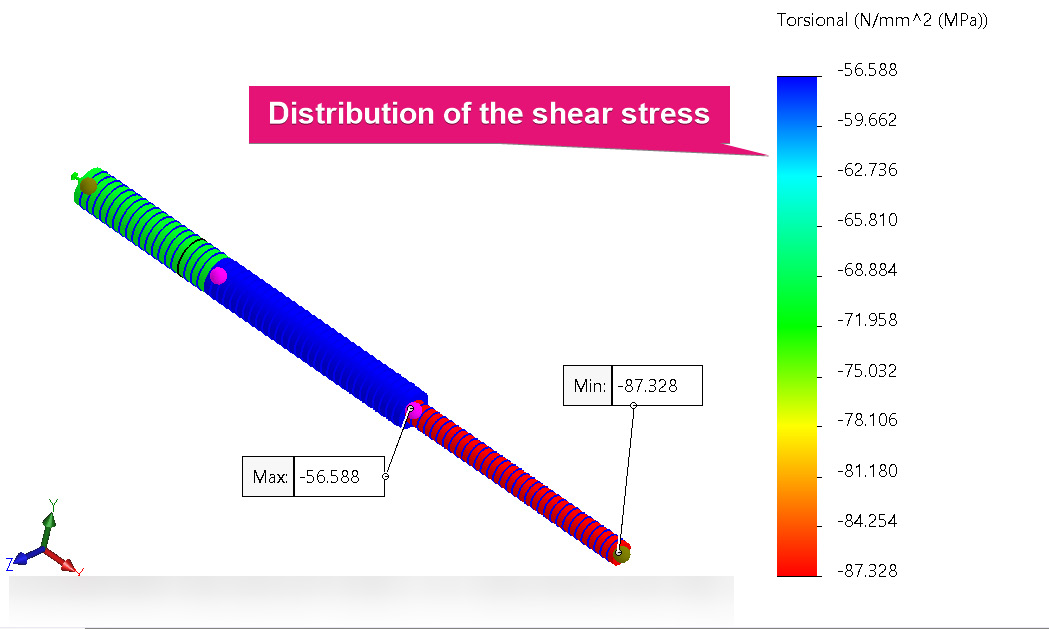
Figure 4.39 – Displaying torsional shear stress

Besides, the negative value of the stress indicates that the segment is under a state of compressive shear stress. In practice, we will want to know whether this stress will cause the component to yield. We may also wish to know the minimum factor of safety within the analyzed component. All of these could be explored further, but our primary objective is simply to demonstrate how to obtain the torsional shear stress value here.

We have now completed the simulation and obtained the answers to the questions posed for the case study of this chapter. The concepts that we have demonstrated using the case study can be extended to many other interesting problems. Some of these problems are highlighted in the next section.

Analysis of components under combined loads

In the example demonstrated so far, we have deployed the beam element for the simulation of a shaft under the influence of torsional loads. Combined with the knowledge of the last two chapters, the procedure we have outlined in the presented example can be easily extended to other problems. For instance, it is a straightforward matter to extend this to components under combined axial plus torsional loads or beams under transverse plus torsional loads. One of the questions in the exercise, inspired by the practical problem proposed in [4], relates to the case of a shaft under combined loads. Furthermore, the approaches we employed in Chapter 3, Analyses of Beams and Frames, and this chapter can also be combined to study grids featuring transverse and torsional loads.

Summary

At the heart of this chapter is a case study that facilitates the exploration of the stress and deformation that stems from the application of torsional loads to an engineering component. Via this case study, we have demonstrated strategies for the following:

• Creating a multi-segment extruded component for simulation purposes
• Creating a custom material from a specific base material
• Applying torsional loads or twisting moments to a component
• Extracting the angle of twist that follows the application of torsional load

With the concepts covered in this chapter (as well as Chapter 2, Analyses of Bars and Trusses, and Chapter 3, Analyses of Beams and Frames), you are now equipped with a few fundamental concepts that can be used to analyze components that can be idealized as one-dimensional members or a collection of one-dimensional members. In the next chapter, we will unveil SOLIDWORKS capability for the analysis of axisymmetric components, which is more advanced than what we have seen up to now.

Exercise

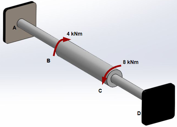
1. Figure 4.40 shows a three-segment shaft used to transmit the two payload torques applied at joints B and C. The shaft is composed of AISI 1010 steel with a shear modulus of 80 GPa. The length LAB = LCD = 200 mm, while LBC = 240 mm. Likewise, segments AB and CD are of diameter 25 mm, while segment BC has a diameter of 50 mm. Use a SOLIDWORKS simulation to evaluate the maximum shear stress in the shaft and then determine the angle of twist of joint C.
   

   Figure 4.40 – A stepped shaft with payload torques

2. Figure 4.41 shows a shaft acting as part of the rotating component of a helicopter. The shaft is under the effect of a combined axial and torsional load, as indicated. The material of the shaft is aluminum alloy 6061, while its cross-section is made of a tube with internal and external diameters of 34 mm and 80 mm, respectively. Use a SOLIDWORKS simulation to determine the maximum shear stress and the maximum von Mises stress.

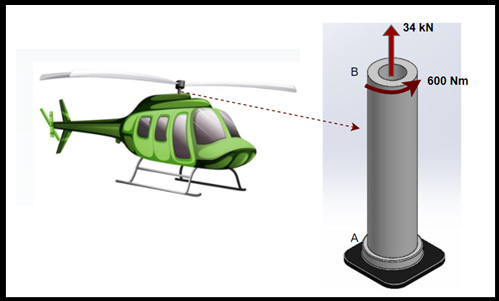
Figure 4.41 – A shaft with a combined axial and torsional loads

References

• [1] Mechanics of Materials, Cengage Learning, B. J. Goodno and J. M. Gere, 2016.
• [2] Mechanics of Materials, McGraw-Hill Education, F. Beer, E. R. Jr. Johnston, J. DeWolf, and D. Mazurek, 2011.
• [3] Mechanical Design of Machine Elements and Machines: A Failure Prevention Perspective, J. A. Collins, H. R. Busby, and G. H. Staab, Wiley, 2009.
• [4] Mechanics of Materials, A. Bedford and K. M. Liechti, Springer International Publishing, 2019.