Chapter 3: Analyses of Beams and Frames

This chapter focuses on the SOLIDWORKS Simulation procedure and strategy for the analysis of transversely loaded members, mainly what we call beams and frames. In our treatment of these structures, we will uncover a few more details about SOLIDWORKS weldment tool, examine how to apply more complex types of load (concentrated load, moment, and distributed load), and explore further computed results that relate to beams. At the end of this chapter, you will become familiar with the procedure and tricks for the simulation of the aforementioned structures. In this vein, the chapter is organized around the following topics:

• An overview of beams and frames
• Strategies for the analysis of beams and frames
• Getting started with analyzing beams and frames in SOLIDWORKS Simulation

Technical requirements

You will need to have access to SOLIDWORKS’ software with a SOLIDWORKS Simulation license.

You can find the sample files of the models required for this chapter here: https://github.com/PacktPublishing/Practical-Finite-Element-Simulations-with-SOLIDWORKS-2022/tree/main/Chapter03

An overview of beams and frames

This section provides basic background information about beams and frames. It highlights their applications, the objectives of simulating/analyzing these structures, and some important technical features relevant to their analysis.

You will likely be familiar with the technical jargons of the mechanics of Solids and its restrictive definition of a simple beam as a structure that satisfies these conditions:

• Capable of supporting transverse loads, which are loads that are applied perpendicular to its length
• Has a length that is far greater than the dimensions of its cross-sections

However, in a more general sense, a beam can support transverse, axial, and torsional loads. But in this chapter, we will only focus on beams supporting transverse loads.

Beams remain one of the most flexible categories of structures used for the design of many engineering products, machines, and systems. You will find them in simple forms, such as a diving board, parallel bars for fitness training, balance beams in gymnastics, lintels that support windows and doors in buildings, and so on. They also exist in more complex forms as part of heavy machinery, medical equipment, vehicles, lifting platforms, buildings, bridges, and so on.

Lengthwise, beams may be designed as a single span, that is, as one long member (as shown in Figure 3.1a), or as a set of continuously connected members (Figure 3.1b). Just like the truss structure we treated in Chapter 2, Analyses of Bars and Trusses (which is a collection of bars arranged to form a larger assembly), we can also bring together a collection of beams and then arrange them to form a bigger assembly that becomes what is known as frames – as reflected in Figure 3.1c and Figure 3.1d:

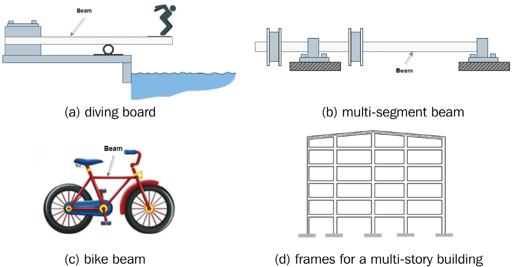
Figure 3.1 – Some applications of beams in practice

When we conduct static analyses of beams and frames, our objectives may center around the following:

• To determine the internal forces and their variations along the length of the members.
• To determine the stresses that developed within the structure or its members (if made up of more than one distinct segment). The stress may be either normal stress caused by the bending moment or shear stress induced by shear forces.
• To evaluate the deformation of the beam or its members (if made up of more than one beam as in the case of connected beams or a frame). A simple beam deformation is characterized by deflection and slope.
• To determine the reaction forces.

As is always the case, the purpose of each of the preceding objectives is to ensure that the beam can support the loads applied to it without premature failure or excessive deformation that will lead to its instability/inability to carry the load.

Important Note

More details about internal loads, types of support, and other details about beams can be found in books on mechanics of solids, such as Hibbeler [1] (see the Further reading section), Bedford and Liechti [2], and others. Nevertheless, recall that if a beam is loaded only by transverse loads, then bending moments and shear forces are the major internal resistant forces in these structures. In a similar spirit, if a beam is loaded by a combination of transverse, axial, and torsional loads, then the internal forces will include bending moments, shear forces, axial, and torsional resistance loads.

The following technical points are worth noting about beams:

• Beams may be long and straight in form, but they may also be curved. However, we will only deal with straight beams in this chapter.
• A beam’s cross-section may be uniform or non-uniform across its length. Simple cross-sections of beams are solid/hollow rectangular sections or solid/hollow circular sections. But the cross-section can also be any of the other standard types shown in Figure 3.2a.
• Some beams will have symmetric cross-sections, while others may have non-symmetric cross-sections. We will focus only on symmetric cross-sections in this chapter.

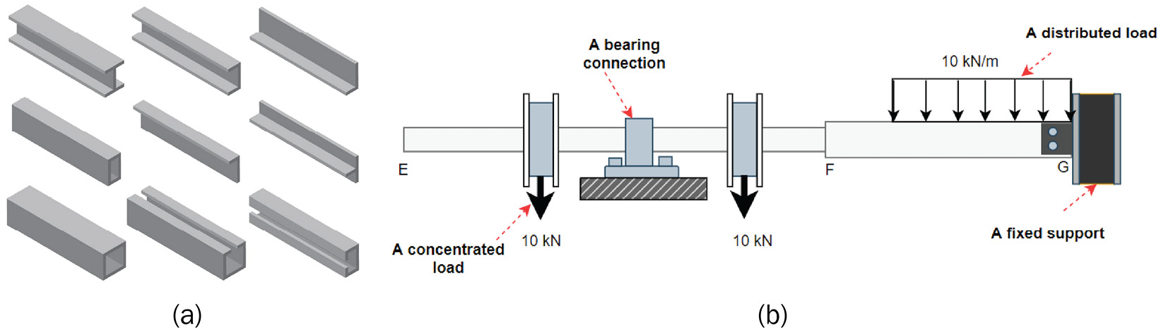
Figure 3.2 – (a) Some typical beam cross-sections; (b) An example of two connected beams with loads and supports

• Some common examples of transverse loads include concentrated forces/moments (acting at a point) and distributed forces/moments (occupying a segment). Figure 3.2b depicts two concentrated forces and a distributed force.

With some of this background information provided about beams, we will briefly highlight strategies for their simulations in the next section.

Strategies for the analysis of beams and frames

This section describes the structural details that are necessary for the analysis of beams and frames. It also highlights the modeling strategy for their simulation and the characteristics of the beam element within the SOLIDWORKS Simulation library.

Structural details

You will need to know the following technical details before venturing into the analysis of beam/frame structures:

• Dimensions

  a. The details of the cross-section

  b. The geometric length of each member

  c. The orientation angles of the members (for a frame)

• The material properties of the beam/members of a frame
• The external loads applied to a beam/frame
• The support provided to a beam/frame to prevent a rigid body motion

Beyond the structural details, we are now set to examine the modeling strategy.

Modeling strategy

Armed with the geometric and material details, the steps to take for the analysis of beams/frames are depicted in Figure 3.3:

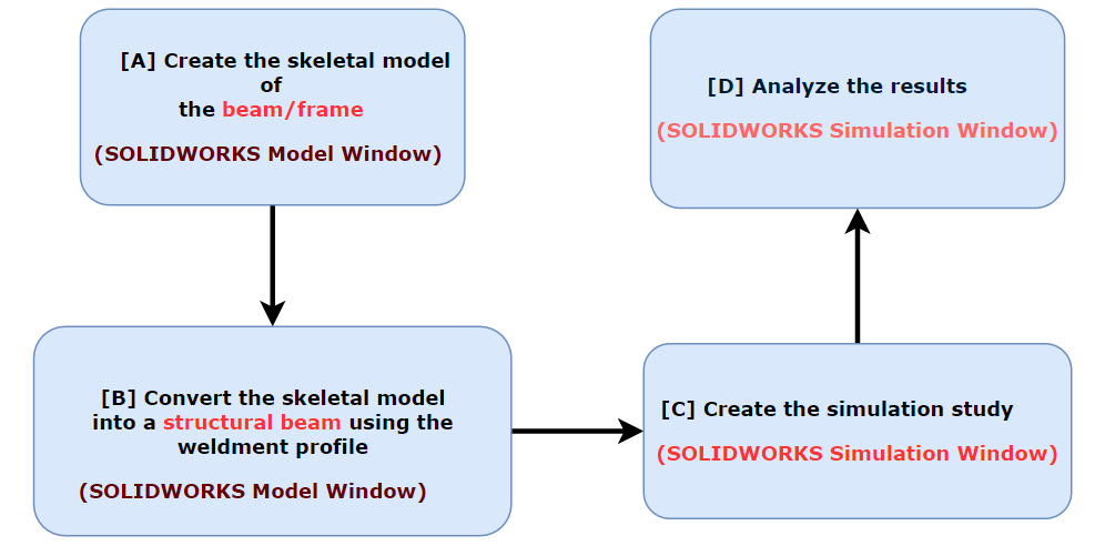
Figure 3.3 – Main steps for the static analysis of beams and frames

There is a subtle difference between this figure and that in Chapter 2, Analyses of Bars and Trusses. Mainly, in step A, we are creating the skeletal model of a beam/frame structure to be simulated. Now, because we will be using the weldments tool, there is an important point you need to know. Primarily, in creating the skeletal line model of a beam-/frame-based structure, you should always consider that there is a virtual joint at critical positions along the length of the beam/frame. These critical positions are located at the following points:

• The beginning and end of a beam
• A point where a concentrated load is applied
• The beginning of a distributed load
• The end of a distributed load
• A point where there is a change of cross-section or change of material properties
• All points of support
• All points of connections

In many practical scenarios, some of these critical points may not be what you would regard as a joint. For instance, to model the beam in Figure 3.4a, a good strategy is to assume the critical positions as shown in Figure 3.4b and then create each of the line segments (AB, BC, CD, DE, EF, and FG) separately before invoking the weldment tool. In a similar spirit, to model the frame structure in Figure 3.4c, we will assume the critical positions as shown in Figure 3.4d and create the necessary line segments (AB, BE, EF, FC, and CD) accordingly:

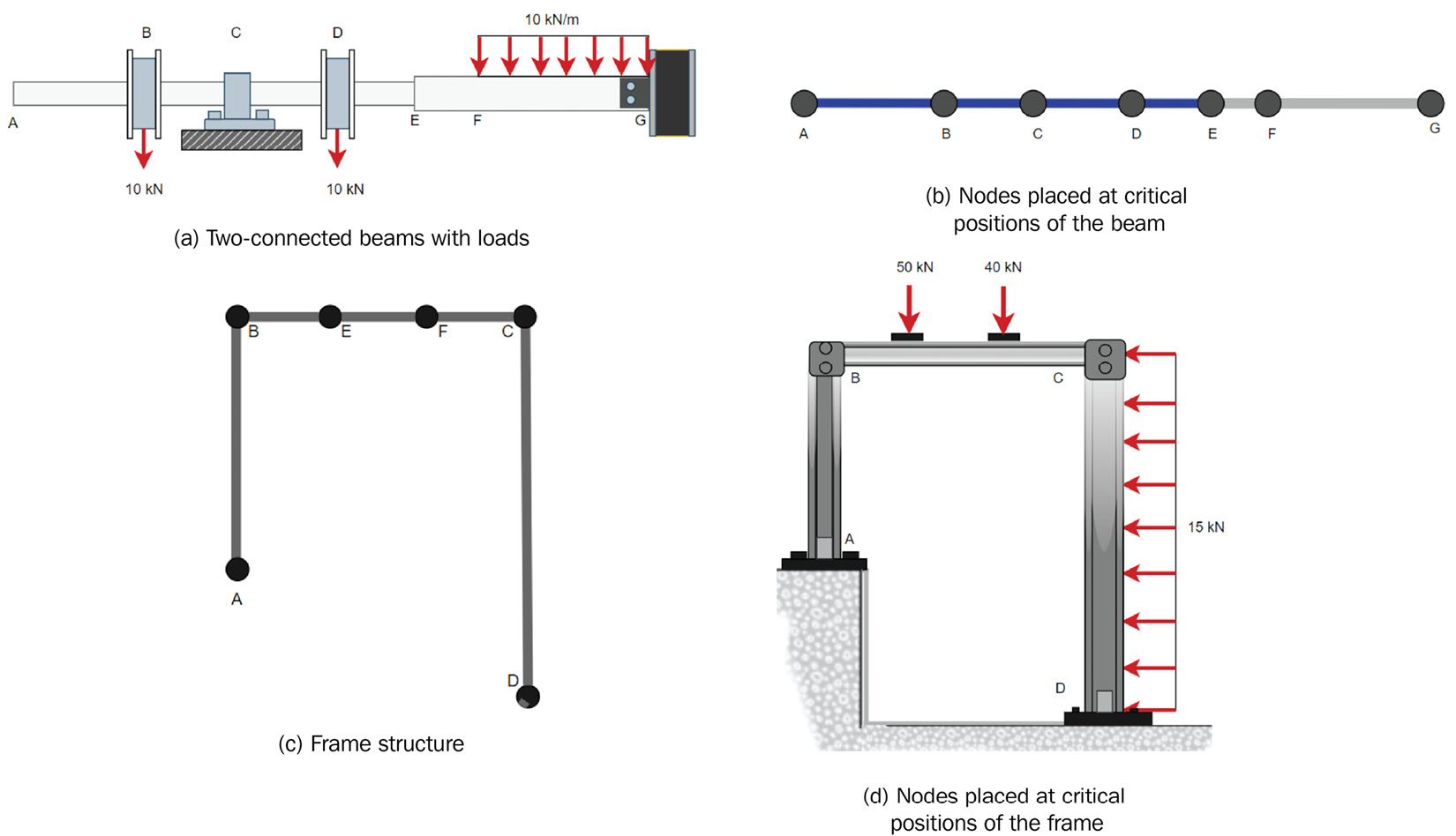
Figure 3.4 – Indication of critical points for modeling beam/frame structures

Notice that points of supports and connections are mentioned among the critical positions listed previously. This indicates that during modeling, the strategy for dealing with different types of support or connections is not to model them directly. Instead, they are represented as joints.

Furthermore, be aware that various types of simple or advanced connections (such as welding, riveting, ball and socket joints, simple thrust bearings, and so on) may be involved in components to be analyzed. A common modeling strategy is to approximate these joints as either fixed/clamped, hinge/simply supported, or roller/sliding support during analysis. Nonetheless, a sound technical judgment of which type of approximation to assign to a connection is necessary.

You will learn more about SOLIDWORKS Simulation features that are used as proxies for each of these types of support in a later segment of this chapter – Part C: Create the simulation study.

With coverage of the modeling strategies out of the way, it is time to reiterate the characteristics of the beam element that we will employ during the simulation case study of this chapter.

Characteristics of the beam element in the SOLIDWORKS Simulation library

Within the SOLIDWORKS Simulation environment, the beam element is used to analyze both beam and frame structures. Like the truss element in Chapter 2, Analyses of Bars and Trusses, the beam element has two nodes. However, there is one major difference. The beam element has six degrees of freedom per node because it is a three-dimensional beam structure. The six degrees of freedom encompass the following:

• Three translational displacements about the x, y, and z axes
• Three rotational displacements about the x, y, and z axes

So far, we have learned about the modeling strategies and the features of the beam element. It is therefore time to go through a case study to explore further details about simulating with this element.

Getting started with analyzing beams and frames in SOLIDWORKS Simulation

In this section, we will demonstrate the use of the beam element with a practical case study that exemplifies a beam carrying multiple types of load.

Through this case study, you will become familiar with how to apply transverse concentrated forces and concentrated moments at a joint. You will also learn how to apply a distributed load on a beam segment. Finally, you will get to see how to extract shear force and bending moment diagrams (which are simulation results that are specific to beams/frames analysis).

Time for action – Conducting a static analysis of a beam with multiple loads

Problem statement

We will analyze the structural component that is loaded and supported as shown in Figure 3.5a. The beam is made of AISI 304 steel and has an S (American Standard) cross-section – S 120 x 12, which is the cross-sectional profile depicted in Figure 3.5b. Using SOLIDWORKS Simulation, we want to accomplish the following tasks:

• Determine the maximum vertical deflection of the beam and the location of this maximum deflection.
• Visualize the variation of shear force and bending moment along the length of the beam.

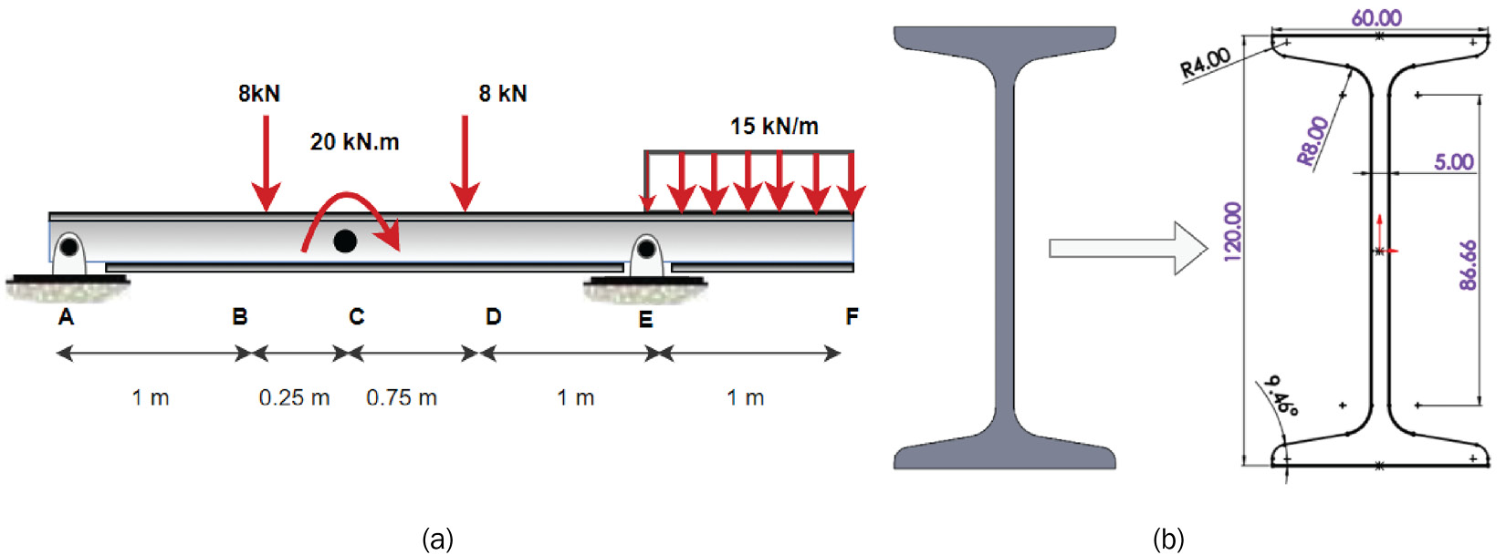
Figure 3.5 – (a) A 2D schematic of a single span beam with multiple loads; (b) An S cross-section profile – S 120 x 12 (unit in mm)

This case study is inspired by a practical problem suggested by Hibbeler [3]. By the end of this simulation study, we will compare the simulation solution we obtained with the partial results provided in [3].

But first, let’s commence the simulation study by initiating the creation of the beam’s model.

Part A – Create a sketch of lines describing the centroidal axis of the beam

As is always the case, creating the geometric model of the structure to be analyzed is the first step in SOLIDWORKS Simulation. in this vein, this section demonstrates the steps to create the geometric line denoting the centroidal axis of the beam.

To begin, start up SOLIDWORKS (File  New  Part) and then create five line segments, AB, BC, CD, DE, and EF, by following the steps highlighted next. Take note that we will sketch the line model of the beam on the front plane.

Let’s get started:

1. Click on the Sketch tab.
2. Click the Sketch tool.
3. Choose Front Plane, as shown in Figure 3.6:

   Important Note

   In structural analysis, there is often a long discussion about the difference between the neutral axis and centroidal axis. The reference to the centroidal axis in this section is used to indicate the line passing through the center of mass of the beam we are analyzing.

   

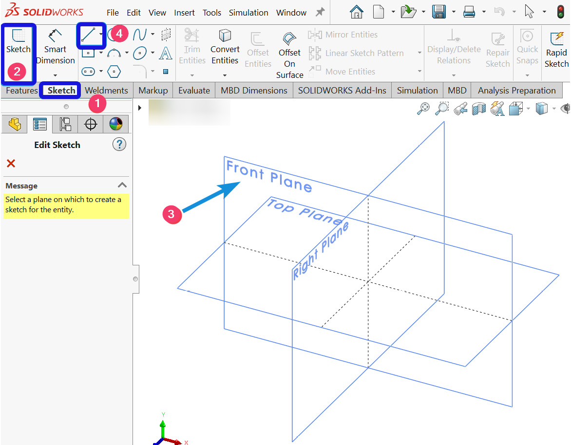
   Figure 3.6 – Initiating the sketch command

4. Select the Line sketching command and create the lines based on the dimensions in Figure 3.7.
5. Click on the Exit Sketch symbol, as indicated in Figure 3.7. Note that exiting the sketch will not close it; it only deactivates the sketching mode.

Figure 3.7 – The sketched line segments

The sketched line we have created represents the centroidal axis of the beam. However, the sketched line has no volume property yet (as we discussed in Chapter 2, Analyses of Bars and Trusses).

In the next section, our objective is to convert the sketched line into a structural model with a volume property.

Part B – Convert the skeletal model into a structural profile

Here, we will convert the sketched lines we created in the preceding section into a structural model using the weldments tool that was introduced in Chapter 2, Analyses of Bars and Trusses.

Activating the weldments tool

Check the set of command items in your SOLIDWORKS CommandManager tabs to see whether the Weldments tab is present. If it is present, then skip the steps here and move to the next sub-section (Adding a structural property).

But if the Weldments tab is absent from the set of CommandManager tabs, then follow the steps highlighted next (summarized in Figure 3.8):

1. Right-click on the CommandManager tab to bring up the option to show more tabs.
2. Move your cursor over the word Tabs.
3. Click on Weldments.

Figure 3.8 – Options to activate the Weldments tab

Once steps 1–3 are complete, the Weldments tab will appear, and we can then make use of the Structural command, as explained in the next subsection.

Adding a structural property

We need to add the cross-sectional profile to the line segments created in the preceding subsection to give it a volume property.

To do this, perform the following steps

1. Click on the Weldments tab, as shown in Figure 3.9.
2. Click on Structural Member.
   

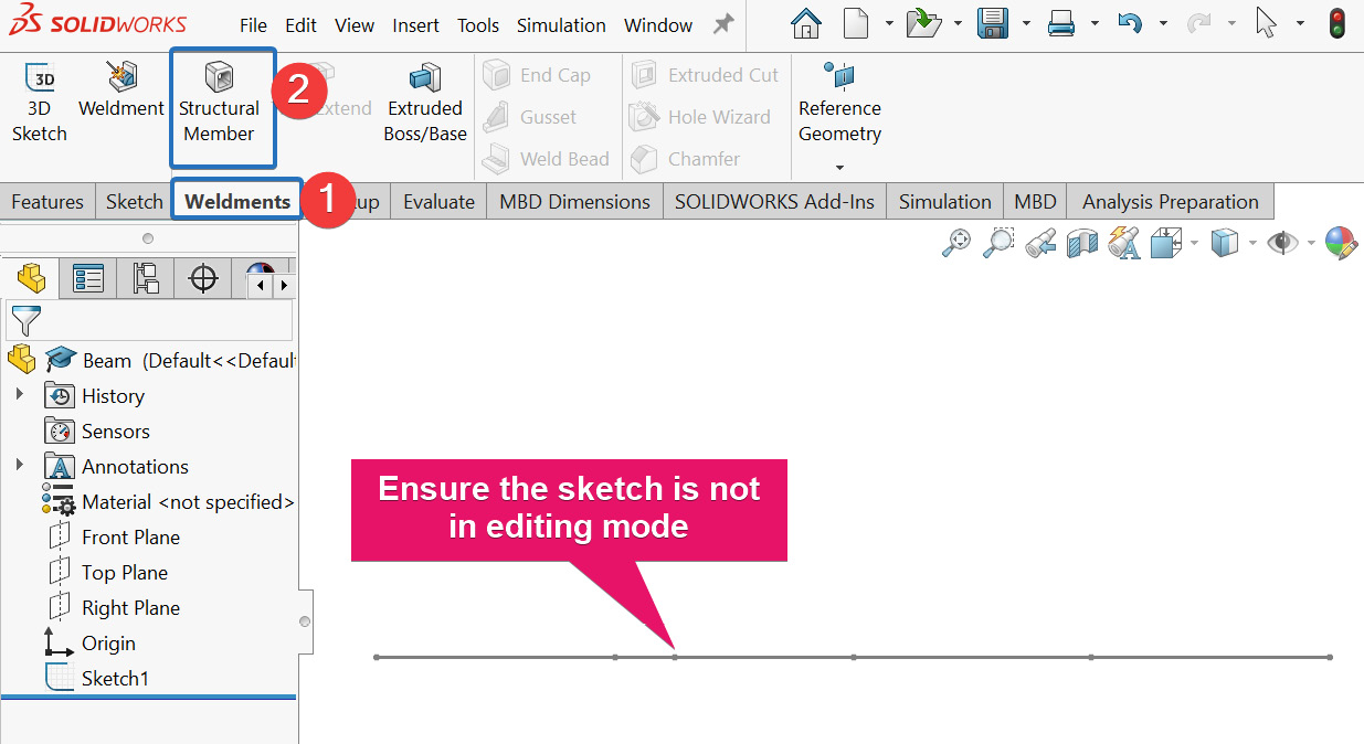
   Figure 3.9 – Beginning the addition of a structural profile

   After completing step 2, the Structural Member PropertyManager window appears, and we now have to make selections of the desired profile from the Simulation library, as documented in Figure 3.10.

3. Under Standard, choose iso (Figure 3.10a).
4. Under Type, select sb beam (Figure 3.10b).
5. Under Size, select 120 x 12 (Figure 3.10c).
   

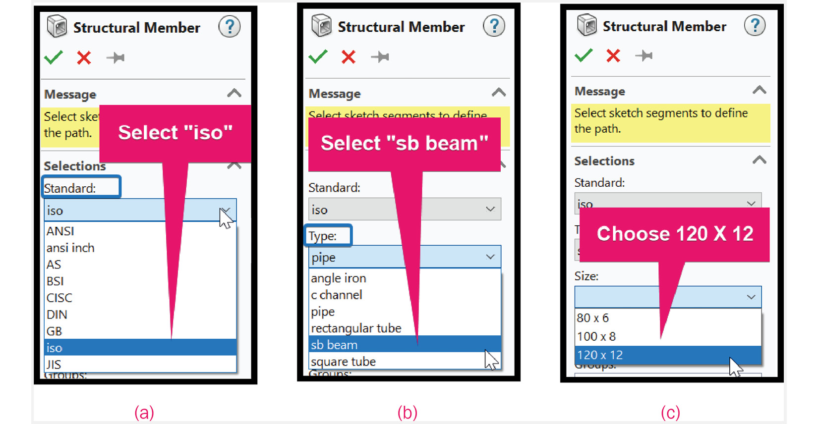
   Figure 3.10 – Selection options for the desired profile

   We still have a few more steps before completing the task in this subsection. Hence, do not close Structural Member PropertyManager yet.

6. Within Structural Member, click New Group to form Group 1 and select all five lines, as shown in Figure 3.11:
   

   Figure 3.11 – Evidence of selecting five line segments

   Before we finish the selection, it is a good idea to check the orientation of the profile to be sure it is what we want.

7. To check and reorient the profile, move to the graphics area and zoom in on the cross-section profile. It is likely to appear as shown in Figure 3.12a. If this is the case, then we have to reorient the profile to stand vertically.
8. Click inside the Rotation Angle box and input 90 deg. This will rotate the profile as demonstrated in Figure 3.12b.
9. Click OK.

Figure 3.12 – (a) Default orientation of the profile; (b) Rotation of the cross-section to the desired orientation

Important Note

Note that it is always necessary to check the orientation of the profile for beam structures as we have done previously. The main reason for this is hinged on the fact that the performance analysis of beam-based structures depends on the second moment of inertia – a geometric parameter that depends on the orientation of the cross-section.

After completing steps 3–9, Figure 3.13 shows a partial view of the solid beam and the changes to the FeatureManager tree:

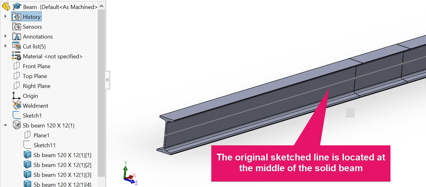
Figure 3.13 – A partial view of the solid beam formed using the Weldment tool

Now that we have converted the sketched line into a collection of solid bodies with a volume property, it is time to bring forth the tools for the analysis.

Part C – Create the simulation study

This section comprises several subsections, each dealing with distinct features of the simulation tasks. The first sub-section deals with the activation steps for the simulation study. This is then followed by a specification of the material for the beam. After this, we will drill down into the application of fixtures and loads. The final subsection relates to the meshing of the structure along with the running of the study to obtain the results.

Let’s go ahead and create the study:

1. Activate the Simulation tab and create a new study.
2. Click on SOLIDWORKS Add-Ins.
3. Click on SOLIDWORKS Simulation to activate the Simulation tab (see Figure 3.14).
   

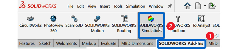
   Figure 3.14 – Activating the Simulation tab

4. With the Simulation tab active, click on New Study (see Figure 3.15).
   

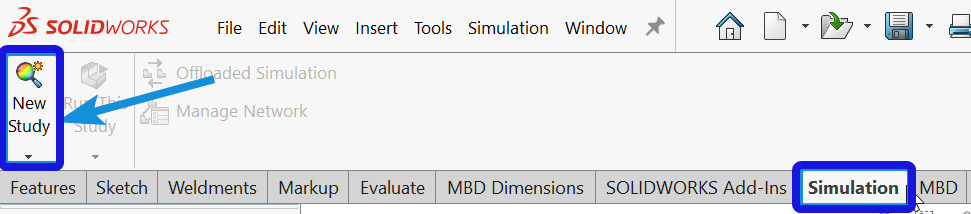
   Figure 3.15 – Activating a new study

   Study PropertyManager appears after step 4 is completed. Within Study PropertyManager, perform the following steps.

5. Input a study name within the Name box, such as Beam analysis.
6. Keep the Static analysis option (as shown in Figure 3.16).
7. Click OK (that is, the green checkmark).

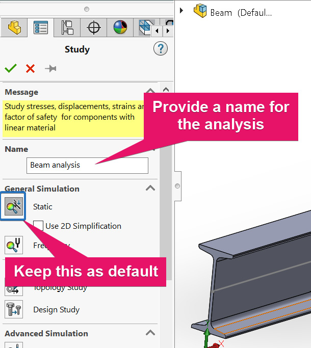
Figure 3.16 – Specifying options for Study PropertyManager

Upon completing steps 4–6, two changes will happen:

• The simulation study tree becomes active (Figure 3.17).
• Joints will be created at the intersection of the beam members and the free ends.

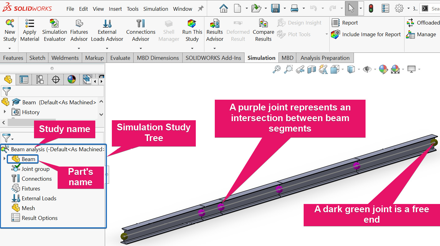
Figure 3.17 – Simulation Study PropertyManager and beam joints

Take note of the two colors used for the joints of the beam depicted in the graphic window of Figure 3.17. The joints in purple represent connections between beam segments, while the dark green joints imply the free ends of the beam.

In the next subsection, we will supply details of the material properties of the beam.

Adding a material property

According to the problem statement, the beam is made of AISI 304 steel, so let’s define the beam’s material property by following these steps:

1. Under the Simulation study tree, right-click on Beam. This brings up the option to select and apply material properties, as shown in Figure 3.18:
   

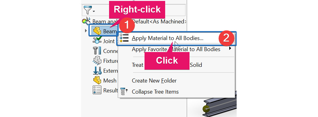
   Figure 3.18 – Activating the material database

2. Click Apply Material to All Bodies.

   Notice that step 2 launches the material database depicted in Figure 3.19. With the Materials window open, perform the following steps.

3. Look for the Steel folder.
4. Click on AISI 304 (see Figure 3.19).
   

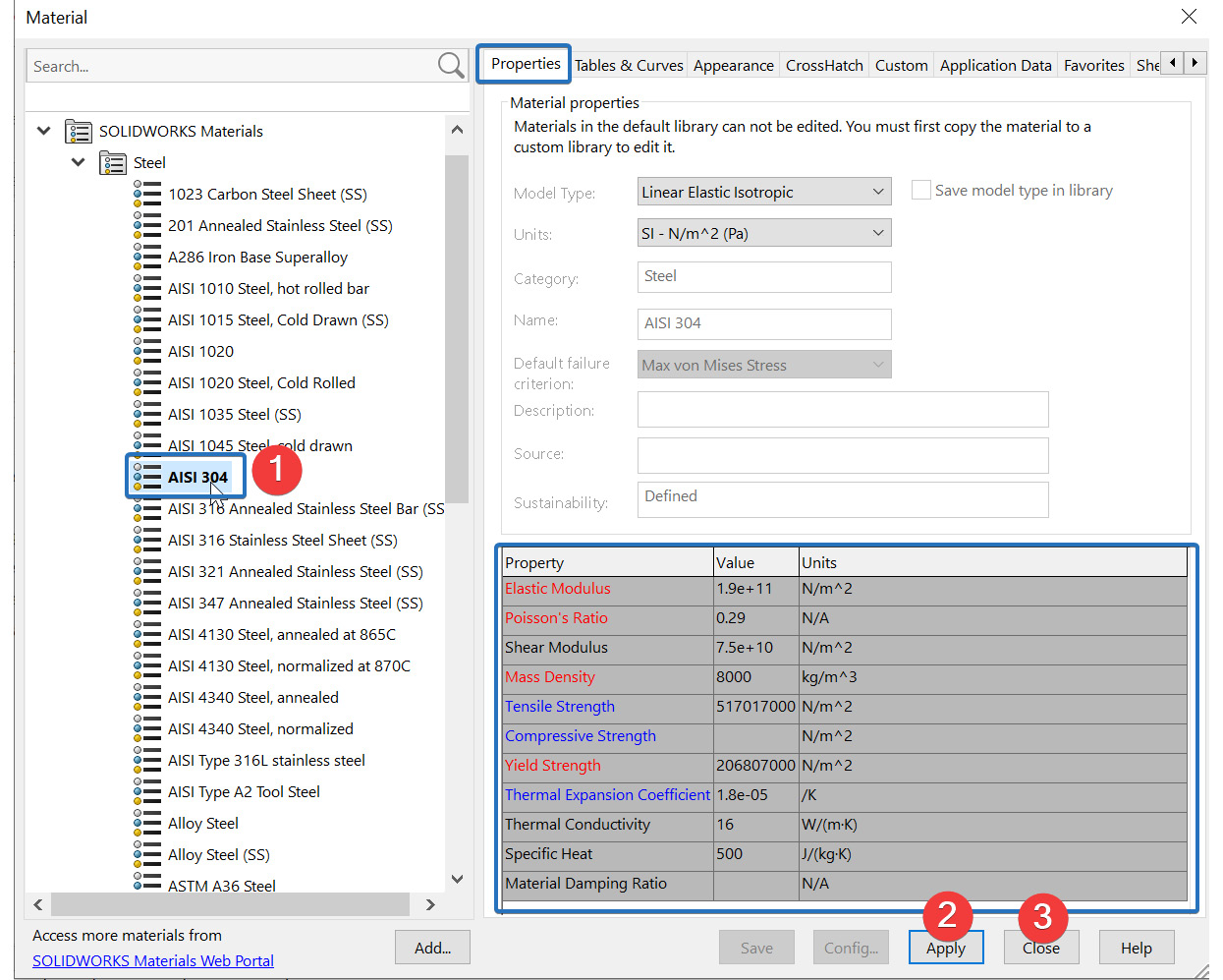
   Figure 3.19 – Options for material specification

   Once you click on AISI 304, its properties will be revealed on the right side of the Material window. From this window, you will observe that some of the property names are in blue font while others are in red or black font (see Figure 3.19). In general, the material properties with names in red font are the ones that must be specified for static analysis. The other property names in blue or black font are either optional for static analysis or needed for dynamic and thermal analyses.

   With this brief detail regarding the Material window, let’s now wrap up the material specification steps:

5. Click Apply.
6. Click Close.

After closing the material database window, a green tick mark () will appear on the part’s name (which we have already explored in Chapter 2, Analyses of Bars and Trusses).

Having completed the material specification steps, it is time to move on to the specification of the beam element to be used for our simulation.

Confirming the beam element status for the segments

SOLIDWORKS Simulation treats a structural member that is created using the weldment tool as a beam by default. Consequently, the software employs the beam element for the simulation of such a structure. The purpose of this subsection is to simply confirm this.

For the confirmation, in the Simulation study tree, do the following:

1. Click on the arrow beside the part’s name to expose the folders named Cut list (see Figure 3.20).
2. Expand the Cut list folder to expose the subfolders named SB BEAM 120.00 x 12.00.
3. Select all the beam segments (each named SolidBody…).
4. Right-click on one of the selected segments, and then choose Edit Definition.

Figure 3.20 – Revealing the structural members' subfolders

Looking closely in Figure 3.20, you will notice that a beam segment (enclosed by a purple ellipse) has a warning sign () attached to its name. This warning is about the shortness of this beam segment and it can be ignored without any issue. We will explore the warning further in Chapter 4, Analyses of Torsionally Loaded Components.

After completing steps 1–4, Apply-Edit Beam PropertyManager will appear:

1. Keep the selection as shown in Figure 3.21.
2. Click OK (the green tick mark) to accept all the default options.

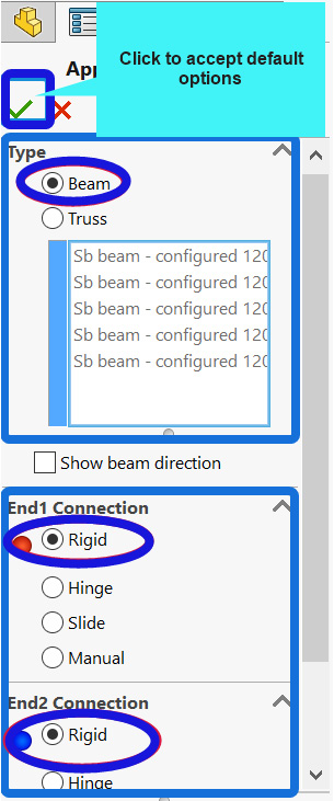
Figure 3.21 – Confirming the beam element selection

You will notice that Beam is selected by default, as shown in Figure 3.21. Furthermore, you will also observe that within Apply-Edit Beam PropertyManager, there are a few possible options to specify the nature of End1 Connection and End2 Connection.

However, the default option that we have gone with here is the Rigid connection for both the End1 and End2 connections. The rigid option indicates that no forces or moments are released at the ends of each beam segment. It is generally the safest option. Proxies for the other options can be specified using the fixture command. Coincidentally, the next section will take us through the process of applying a fixture.

Applying a fixture

Fixtures are used to prevent engineering structures from excessive unstable movement when loads are applied to them.

For the problem we are analyzing, the supports found at locations A and E (as indicated in the problem statement – Figure 3.5a) represent the fixtures. You will notice that the two supports are pin connections. Each pin connection will act to prevent the three translational movements along the x, y, and z axes at each joint.

We will apply the two fixtures in the same set of steps because they are of the same nature. Consequently, to apply the fixture at joints A and E, follow these steps.

Under Simulation study tree, do the following:

1. Right-click on Fixtures, and then pick Fixed Geometry from the context menu that appears (Figure 3.22).
   

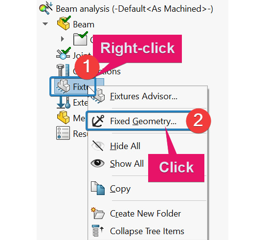
   Figure 3.22 – Activating Fixture PropertyManager

2. Under Fixture PropertyManager (Figure 3.23), select Immovable (No translation).
3. Move the cursor into the graphics window and pick joints A and E.
4. Click OK.

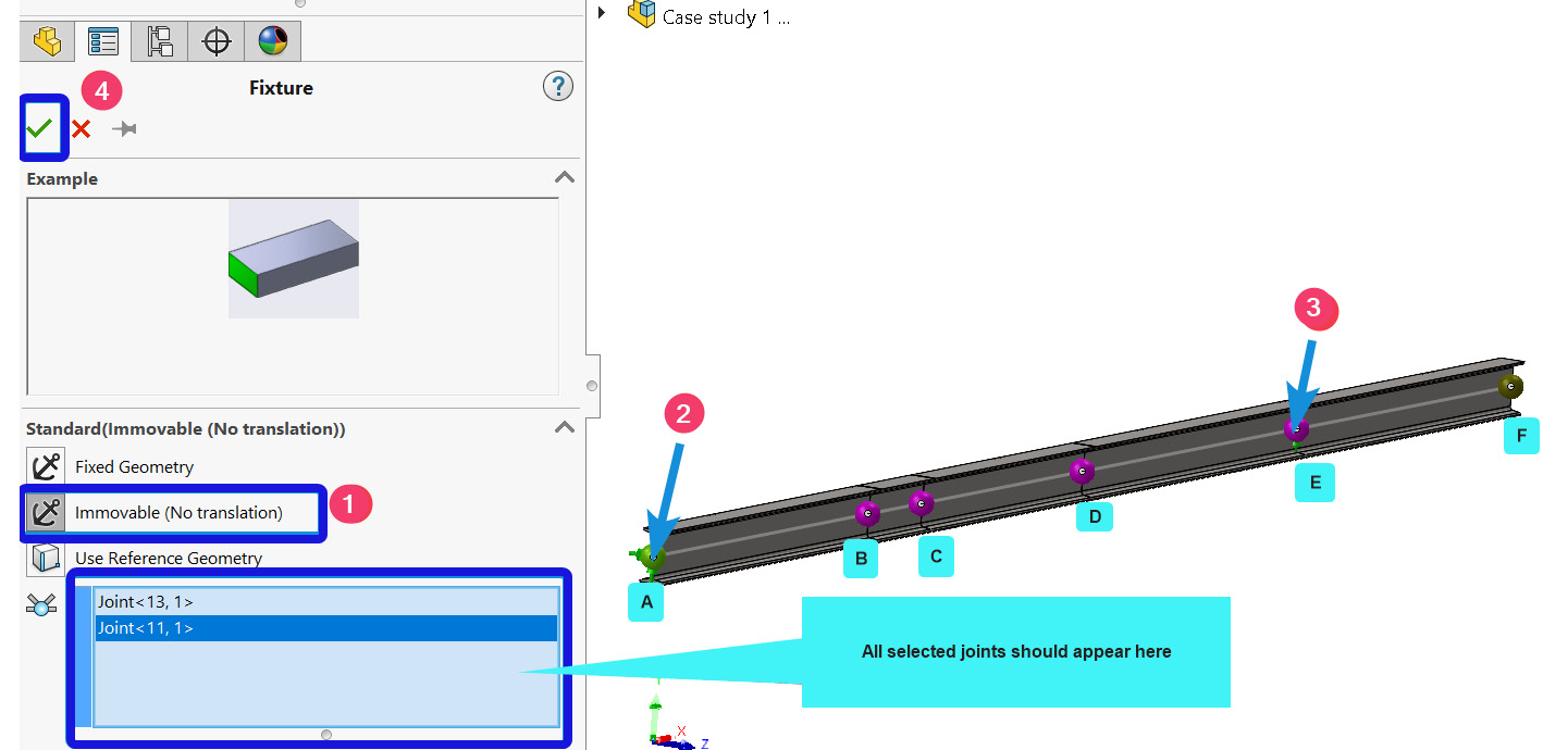
Figure 3.23 – Selecting the immovable fixture for joints A and E

Important Note

Note that in many other practical analysis cases, you may have a combination of support types that perform different functions, such as fixed support and a pin connection at different positions. In those cases, you will need to apply each fixture one at a time, not at once, as we have done previously by selecting joints A and E in one single set of steps.

It bears pointing out that SOLIDWORKS Simulation provides commands to apply the three most common types of supports when dealing with beams. Let’s cycle through these prominent supports before moving on to the next subsection:

• Fixed/clamped support – This type of support prevents the three translational movements and the three rotational displacements when applied to a joint. In SOLIDWORKS Simulation, this type of support is handled by the fixture type called Fixed Geometry.
• Pin/hinge/simply support – This kind of support prevents all three translational movements at a joint. Within the SOLIDWORKS Simulation environment, this type of support is handled by the fixture indicated by Immovable (No translation).
• Roller support – This type of support prevents a limited number of translational displacements of a joint. Within the SOLIDWORKS Simulation environment, we tackle this type of support by using the Use Reference Geometry fixture type.

Of course, apart from the three common support types mentioned previously, there are also others. This includes elastic support and sliding support. We can apply sliding supports on a beam’s joint using the Use Reference Geometry fixture type. However, take note that SOLIDWORKS Simulation only allows the application of elastic support for a solid/shell element.

We now turn to the application of the external loads in the next subsection.

Applying loads

We have three types of loads that are externally applied to the beam, as revealed in the following problem statement:

• Concentrated payload weights at positions B and D
• A concentrated moment at position C
• A uniformly distributed load (UDL) occupying segment EF

The steps to apply to each of these loads are discussed next. We will start with the concentrated loads, then the moment load, and finally we will apply the UDL.

Applying the concentrated loads at joints B and D

Under Simulation study tree, perform the following steps:

1. Right-click on External Loads, and then select Force (as shown in Figure 3.24).
   

   Figure 3.24: Activating Force/Torque PropertyManager

   Within Force/Torque PropertyManager, perform the following steps.

2. Under Selection, click on the Joints symbol (labeled 1 in Figure 3.25).
3. Navigate to the graphics window and pick joint B.
4. Click inside the load reference box (labeled 3 in Figure 3.25).
5. Expand the FeatureManager tree to select Front Plane as the reference plane.
6. Under Force, activate the vertical force component box and input 8000 (ensure the unit is set to an SI unit).
7. Check Reverse direction (labeled 7 in Figure 3.25). This changes the force direction to downward.
8. Click OK.

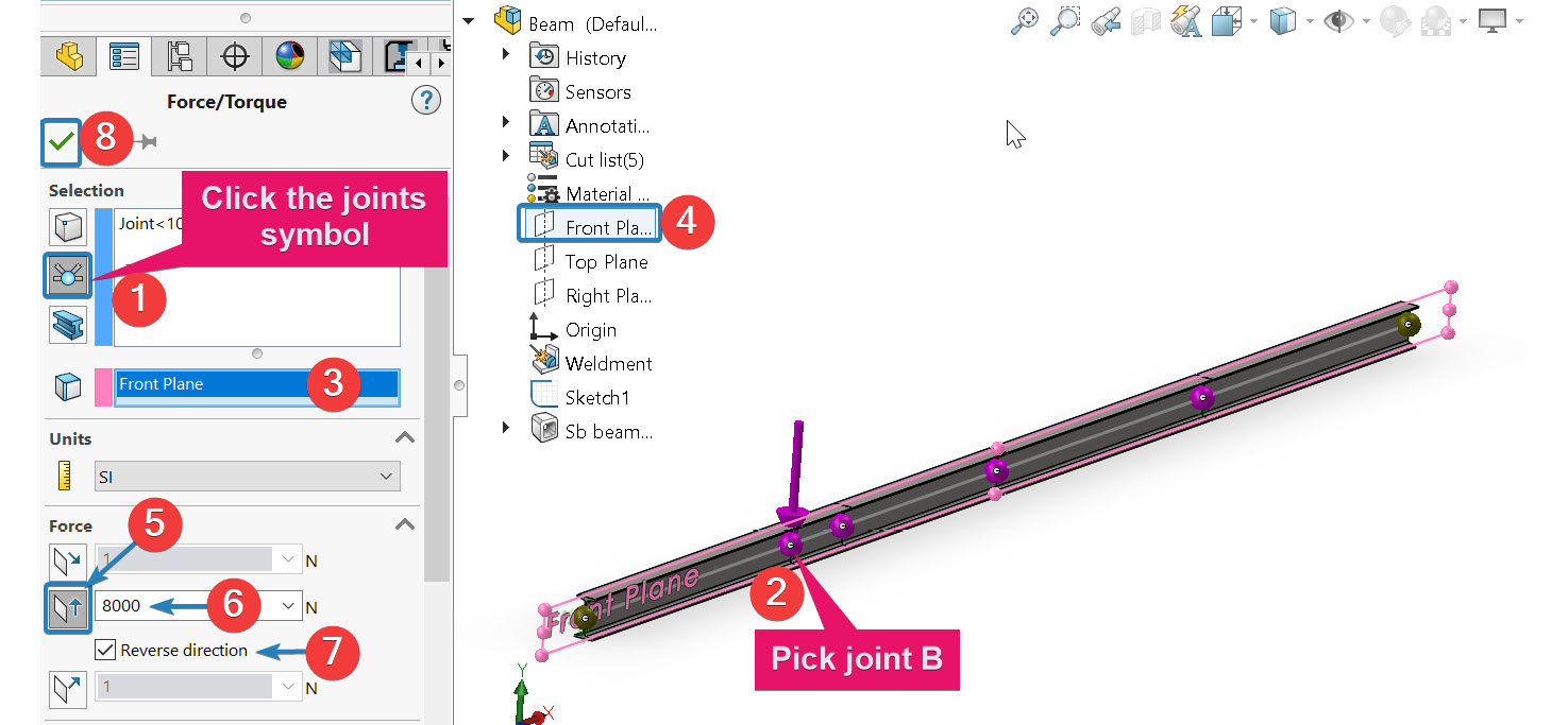
Figure 3.25 - Applying a concentrated force at joint B

You will notice that Force/Torque PropertyManager has five areas:

• Selection – This is used for specifying geometry on which a load is applied.
• Units – This is used for indicating the desired unit of the load we are applying.
• Force – This section is for specifying the magnitude and direction of a force.
• Moment – This section is for specifying the magnitude and direction of a moment.
• Symbol Settings – This is valuable for increasing the size of the arrow representing a load. Usually, the arrow that signifies a load may be too small. See Figure 3.26 on how to modify the size and color of the arrow.

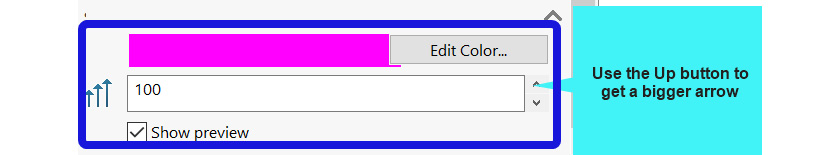
Figure 3.26 – Editing the size and color of a load’s arrow symbol

Repeat steps 1–8 to apply the 8000 N force on joint D. However, remember to select joint D in step 3.

Applying the concentrated moment at joint C

We are now set to apply the moment at joint C. Before we do that, there are three things to take note of when dealing with the load type called moment:

• First, in most engineering mechanics textbooks, it is typical to employ a curved arrow to represent an externally applied moment (as illustrated in Figure 3.5a). However, within SOLIDWORKS Simulation, the symbol used to represent a moment appears as a nail, as you will see later in this subsection.
• Second, SOLIDWORKS Simulation employs a convention that holds that a counterclockwise moment is positive, while a clockwise moment is negative.
• Third, a moment applied to a point will need a reference plane. Selecting the right reference plane for a moment is not as intuitive as that of a force. So, care should be taken in the steps involved in specifying the reference plane of the moment.

With the preceding background information, let’s now shift our attention back to applying the moment at joint C by following the steps spelled out next.

Under Simulation study tree, do the following:

1. Right-click on External Loads and select Force.
2. Within Force/Torque PropertyManager, follow the options highlighted in Figure 3.27:

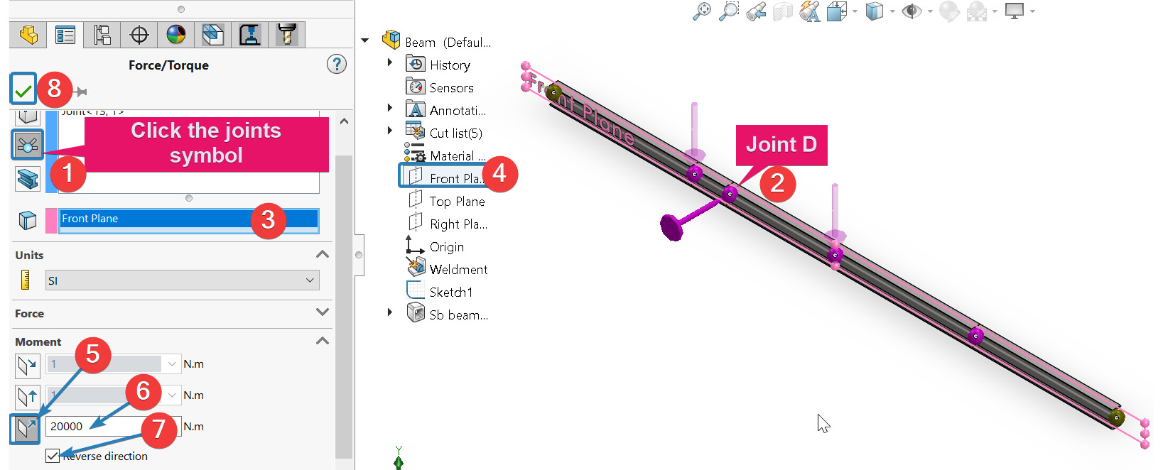
Figure 3.27 – Options for applying a concentrated moment at joint C

Notice that the action labeled 7 in Figure 3.27 invokes the Reverse direction command. This step is necessary to ensure that the applied moment is negative in compliance with the problem statement. In addition to this, you will see that the symbol of the moment aligns with the Z axis.

As you have seen so far, concentrated forces and concentrated moments act at a joint. But we could also have loads that will act on a segment, rather than on joints. This load type is called a distributed load and it is the focus of our next action.

Applying the distributed load on segment EF

In the final step for this subsection, we will apply a distributed load on segment EF of the beam.

Under Simulation study tree, do the following:

1. Right-click External Loads and select Force.
2. Within Force/Torque PropertyManager, follow the steps highlighted in Figure 3.28:

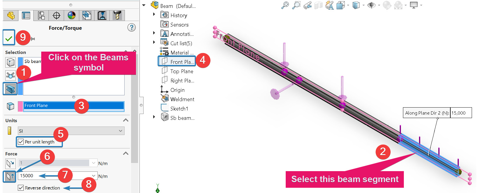
Figure 3.28 – Applying a distributed load on segment EF of the beam

After completing the preceding steps, the appearance of the model in your graphic window should be as shown in Figure 3.29 (viewed isometrically). Notice the symbols representing the concentrated forces at points B and D. Also take note of the concentrated moment at point C and the distributed load on segment EF of the beam. Additionally, pay attention to the support at joints A and E.

Figure 3.29 – Appearance of the different external loads

We have now completed the application of the three loads. We will be creating and running the mesh in the next subsection.

Meshing and running

We are getting close to completing the preprocessing steps. Meshing is a crucial step of the finite element simulation. As previously mentioned in Chapter 2, Analyses of Bars and Trusses, the two approaches for creating a mesh in SOLIDWORKS Simulation are Create Mesh and Mesh and Run. In this subsection, we will be using the second approach, which combines the meshing and running of the analysis in a single step. The method works well when analyzing components with either truss or beam elements. Be aware that when this method is used for the structure we are analyzing, it will create an element between two joints. Besides, we do not have to do detailed mesh refinement for this problem because of the strategic use of critical positions employed in creating the geometric model of the beam in the section named Part A – Create a sketch of lines describing the centroidal axis of the beam. As you will later see in Chapter 5, Analyses of Axisymmetric Bodies, and Chapter 6, Analyses of Components with Solid Elements, for more advanced analysis, a mesh convergence study will be crucial to get accurate results.

For our next action, perform the following steps:

1. Right-click on Mesh.
2. Select Mesh and Run (as highlighted in Figure 3.30).

Figure 3.30 – Activating the meshing and running options

After completing steps 1 and 2, the study tree and graphics window will appear, as shown in Figure 3.31a and Figure 3.31b, respectively:

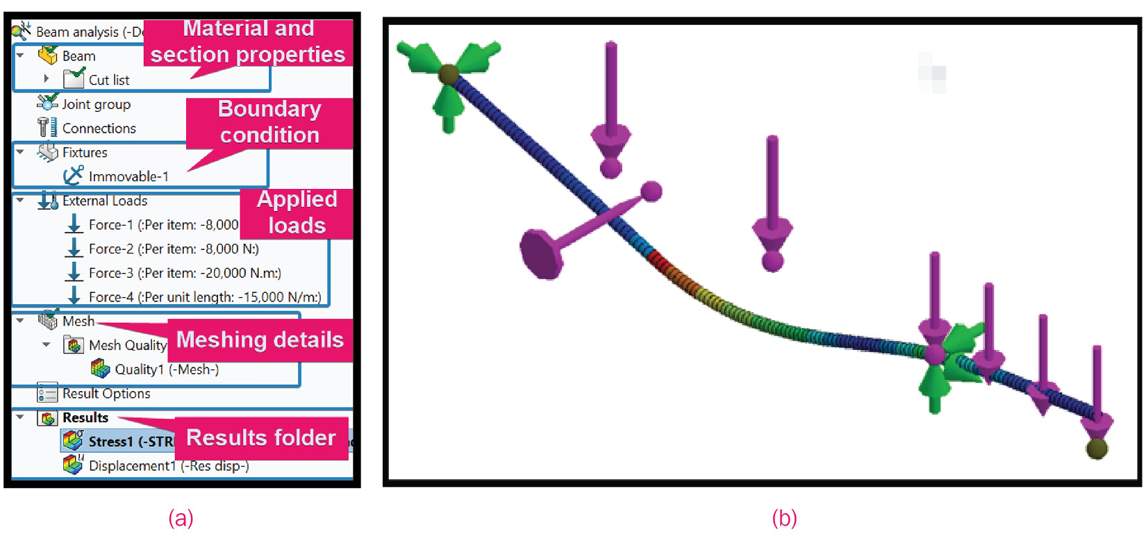
Figure 3.31 – (a) An annotated appearance of the simulation study tree after completing all the steps; (b) A partial view of the graphics area

Up to this point, we have created a sketched line of the beam and converted the sketched line into a series of structural members with volume properties using the weldment tool. Furthermore, we have specified the material property, applied fixtures, and specified three different types of loads. Besides that, we have created the mesh and run for our analysis. It is now time to conduct a post-processing analysis of the simulation results, which is what the next section is about.

Part D – Examining the results

In this section, we will address the following questions that were part of the problem statement:

• What is the maximum vertical deflection of the beam and the location of this maximum deflection?
• What is the graphical variation of the shear force and the bending moment along the length of the beam?

Let’s start with the first question about obtaining the maximum deflection.

Obtaining the maximum vertical deflection of the beam

To retrieve the maximum deflection experienced by the beam, perform the following steps:

1. Right-click on Results, and then select Define Displacement Plot (Figure 3.32).
   

   Figure 3.32 – Activating Displacement Plot PropertyManager

   This opens up Displacement Plot PropertyManager, as shown in Figure 3.33:

   

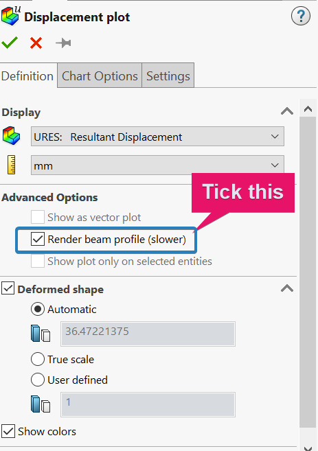
   Figure 3.33 – Displacement Plot PropertyManager

   You will notice that Displacement Plot PropertyManager has three tabs:

   a. Definition

   b. Chart Options

   c. Settings

   Various customizations can be done to our results using each of these tabs as follows.

   Within Displacement Plot PropertyManager, select the following options (summarized in Figure 3.34):

2. Under the Definition tab, select UY: Y Displacement (Figure 3.34a).
3. Move to the Chart Options tab, under the Display options, and check the Show min annotation and Show max annotation boxes. While still within the Chart Options tab, under Position/Format, change the number format to floating for a more readable display of the numerical values (Figure 3.34b).
4. Move to the Settings tab and, under Boundary Options, check the Superimpose model on the deformed shape box, and then click OK (Figure 3.34c).

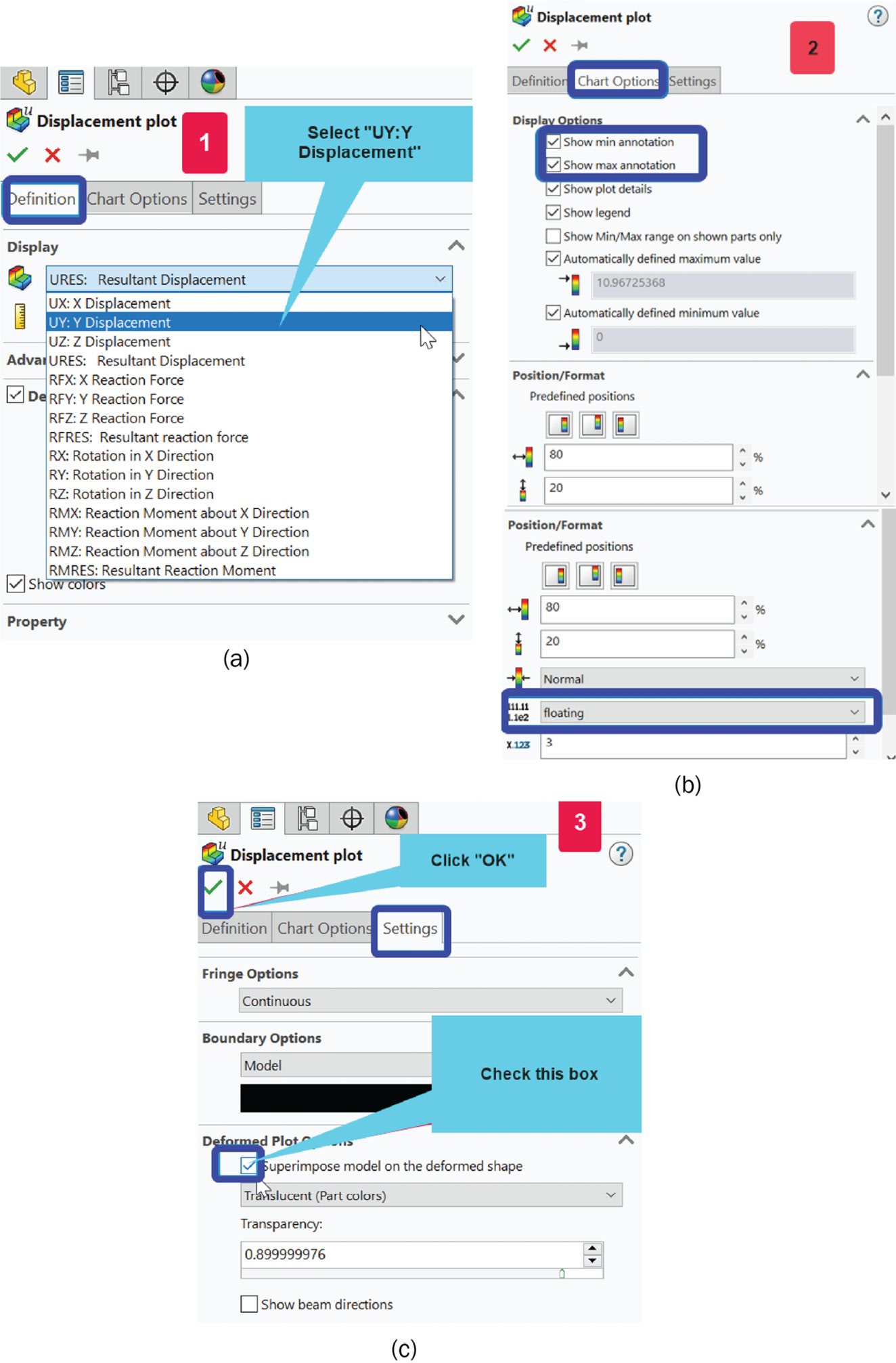
Figure 3.34 – Selecting the options for the displacement result along the Y axis

After completing steps 1–3, the graphic window will be updated with the displacement plot. Figure 3.35 depicts the deflected shape of the beam (viewed in the front plane). From this figure, we can see that the beam experiences a maximum deflection value of 10.967 mm (downward) at a point to the right of point C:

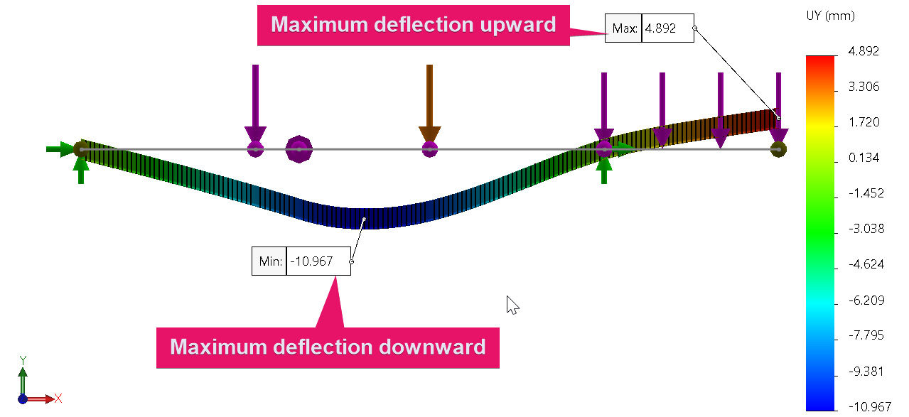
Figure 3.35 – The deflected shape superimposed on the undeflected shape of the beam (front view)

To check whether this maximum deflection value is acceptable, one rule of thumb (depending on the professional code) is to consider whether the maximum deflection value exceeds L/240, where L is the length of the beam. Going by this, since the length of our beam is L = 4 m, then L/240 = 16.67 mm. Therefore, the conclusion is that since L/240 is greater than the maximum deflection we found in the simulation, the deflection of the beam is relatively acceptable. Nonetheless, take note that the value of the maximum deflection must be used together with other stress-based failure criteria to make the right judgment about the safety of the beam.

Important Note

For a further discussion of deflection limits, you can check Chapter 9, Simulation of Components under Thermo-Mechanical and Cyclic Loads, in the book by Mott and Untener [4]. However, for more in-depth coverage of failure theories in the context of designing engineering structures, you can consult the books by Collins, et al. [5] and Brown [6].

Beyond the knowledge of the maximum deflection, it is also desired to examine the visual variation of the internal resistance loads within the beam, which is what we will do next.

Obtaining the shear force and bending moment diagrams

In this subsection, we will obtain the visualization of the internal forces.

For simple beams that are loaded with just transverse forces, the internal resistant loads take the form of shear force and a bending moment. These internal resistance loads are technically responsible for the stresses that develop within beams/frames. This means that by knowing the variation of these internal resistance loads, we can graphically locate a segment of the beam/frame that will be susceptible to high stress. In practice, information about the highly stressed segment can be deployed to decide upon the segment of the beam that needs to be reinforced with more materials.

In what follows, we will start with an examination of the shear force diagram and then proceed to examine the bending moment diagram.

Shear force along the entire span of the beam

Let’s generate a visualization of the shear force variation along the span of the beam:

1. Right-click on Results, and then select Define Beam Diagrams (Figure 3.36).
   

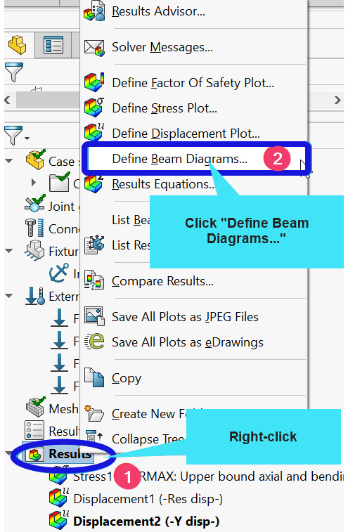
   Figure 3.36 – Activating Beam Diagrams PropertyManager

   Within Beam Diagrams PropertyManager, select the following options (summarized in Figure 3.37):

2. Under the Definition tab, select Shear Force in Dir1 (Figure 3.37a).
3. Move to the Chart Options tab, under Display Options, and check the Show min annotation and Show max annotation boxes. While still within the Chart Options tab, under Position/Format, you should change the number format to floating for a more readable display of the numerical values (Figure 3.37b).
4. Click OK.
   

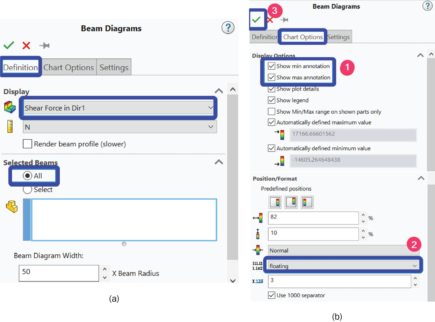
   Figure 3.37 – Beam diagrams selection for shear force

5. In the graphic window, change the view orientation to Front View (Figure 3.38):

Figure 3.38 – Updating the view orientation to Front View

Once steps 1–5 are complete, the graphic window will be updated to reveal the variation of the shear force along the length of the beam, as shown in Figure 3.39:

Figure 3.39 – The variation of shear force along the entire beam

The numerical values of shear force and the distribution of these values are indicated in the color legend beside the plots. As you can see from the plot, segment EF (carrying the distributed load) is under the effect of negative shear forces (compression), while the other segments are under the influence of positive shear forces.

In the preceding steps, we have obtained the shear force diagram for the entire length of the beam. However, it is also possible to obtain the shear force diagram for a partial segment of the beam. Indeed, in [3], only a partial solution is provided for this problem. This partial solution indicates that the value of shear force immediately to the right of the 1 m position (measured from the left end) or simply to the right of segment AB is 9.17 kN. Also, the value of the shear force immediately to the right of the 3 m position (measured from the left end) is reported as -15 kN.

To compare our simulation results with these values, we need to obtain the variation of shear force in only partial segments of the beam. This is done as follows:

1. Right-click on Results, and then select Define Beam Diagrams (similar to Figure 3.36).

   Within Beams Diagram PropertyManager, perform the following steps.

2. In the Definition tab, under Display, select Shear Force in Dir1 (Figure 3.40a).
3. In the Definition tab, under Selected Beams, click on Select, and then pick segment 2 and segment 5 in the graphic window.
4. Move to the Chart Options tab to pick the options shown in Figure 3.40b
5. Click OK.
   

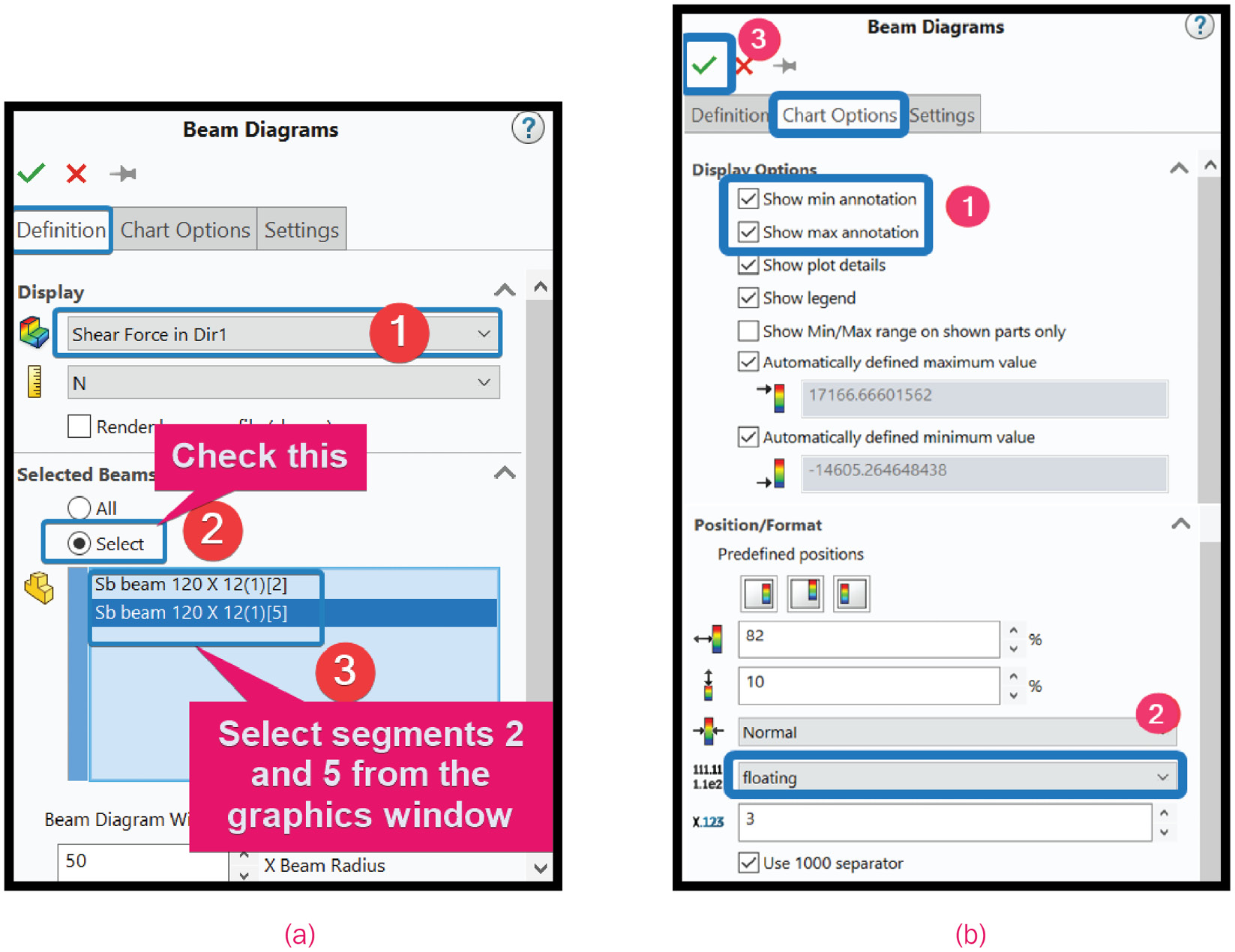
   Figure 3.40 – Options for the beam diagrams concerning a partial view of the shear force diagram

6. In the graphic window, change the view orientation to Front View.

With the completion of steps 1–6, the graphic window is updated to show the variation of shear force over segments 2 and 5 of the beam, as shown in Figure 3.41:

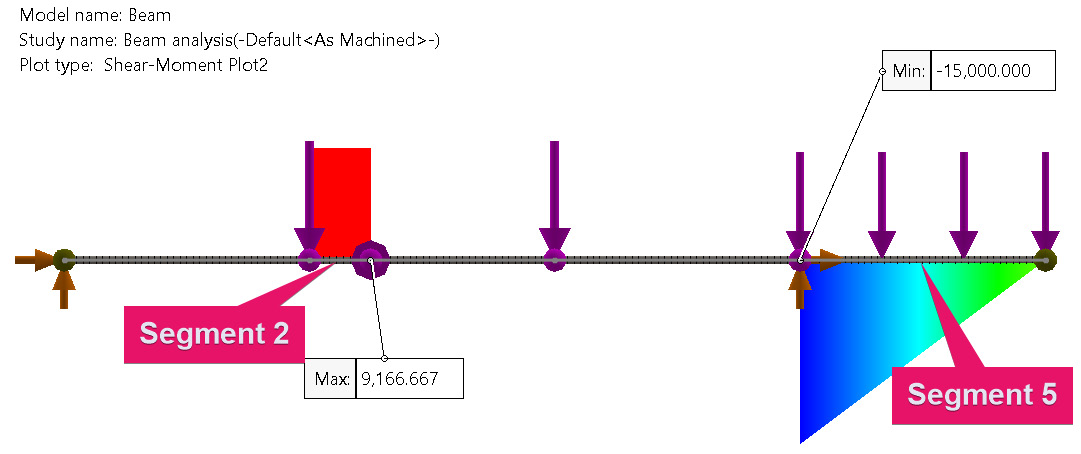
Figure 3.41 – Shear force diagram for two selected segments of the beam

From Figure 3.41, you can observe that the shear force to the right of the 1 m and the 3 m marks is 9166.67 N (which approximately equals 9.17 kN) and -15000 N (which approximately equals 15 kN), respectively. This shows that there is a good agreement between our simulation results and that reported in [3].

This now completes our evaluation of shear force and its variation along the length of the beam. Next, we move on to the graphical evaluation of the bending moment.

Obtaining the bending moment over the entire length of the beam

To visualize the variation of the bending moment along the entire span of the beam, follow these steps:

1. Right-click on Results, and then select Define Beam Diagrams (similar to Figure 3.36).
2. Within Beam Diagrams PropertyManager, in the Definition tab, under Display, select Moment about Dir2 (Figure 3.42a).
3. Move to the Chart Options tab to pick the options shown in Figure 3.42b:
   

   Figure 3.42 – Options for Beam Diagrams PropertyManager concerning the bending moment diagram

4. Change the view orientation to Top View (as shown in Figure 3.43).

Figure 3.43 – Changing the view orientation to Top View

Figure 3.44 shows the variation of the bending moment. The figure indicates that immediately to the right of the 3 m position, the bending moment value is 7500 Nm, which matches what was reported in [3]. Again, the distribution of the variation of the bending moment values is indicated in the color legend beside the plot.

Figure 3.44 – The variation of the bending moment diagram over the entire beam

Just to reiterate, the importance of both the shear force and bending moment diagrams is to investigate the region/segment of the beam that is heavily strained. Once such a region is determined, the information can be used to reinforce the beam and hence increase its strength accordingly.

This now wraps up the solution to the questions posed for the case study. As you will have noticed, many more results can be obtained and examined depending on our objectives. As we continue our exploration in the coming chapters, we will be uncovering other important features of interest.

The concepts that we have demonstrated using the case study can be extended to many other interesting problems, as we will see in the following section.

Analysis of plane and space frames

In the case study demonstrated so far, we have deployed the beam element within the SOLIDWORKS Simulation library to simulate the structural behavior of a beam structure with different types of loads. The procedure outlined in the presented case study is perfectly suitable to study two-dimensional/plane frames. This is because a plane frame is just a collection of beam structures oriented in the two-dimensional plane. The exercise section contains a question on the extension of the beam element for the analysis of frames and a complete solution is available for download. Additionally, the procedure of this chapter is also suitable to study three-dimensional or what we generically call space frames. However, for this, we need to make a simple adjustment to Part A of the procedure (creating the skeletal lines). What does this modification involve? Basically, in the case of space frames, the skeletal lines must be situated in a 3D space, which is relatively easy if you have familiarity with SOLIDWORKS modeling. A problem on this is included in the exercise and a complete solution file is available for download.

Summary

In this chapter, we have explored the fundamental procedures involved in the static analysis of beams. Building on our knowledge of the weldment tool introduced in Chapter 2, Analyses of Bars and Trusses, we have demonstrated how to create the model of a beam and the transformation of the model into a beam structural member. Beyond this, the chapter entails additional knowledge that relates specifically to the simulation of beams. Some of these include the following:

• How to employ critical points along the length of the beam to create the line segments
• How to rotate a weldment profile to achieve the desired orientation
• How to apply a distributed load on a beam segment
• How to apply a moment at a point on a beam and the SOLIDWORKS Simulation convention
• How to extract the maximum deflection of a beam
• How to visualize the shear force and bending moment diagrams

You saw how to handle the simulation of trusses and beams/frames in Chapters 2, Analyses of Bars and Trusses and Chapter 3, Analyses of Beams and Frames, respectively. In the next chapter, you will learn about the analysis of components loaded with torques, and in doing so, you will familiarize yourself with how to use the beam element without employing the weldment tool.

Exercises

1. Figure 3.45 shows a beam made of ASTM-A36 structural steel with a triangularly distributed load. The beam is made of S (American standard) cross-section – S120 x 12. Use SOLIDWORKS Simulation to evaluate the shear force and bending moment diagrams.
   

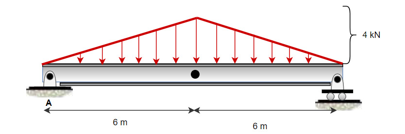
   Figure 3.45

2. Figure 3.46 shows 2D schematics of two bicycle frames that are to be compared for structural performance. The frames are made of aluminum alloy 6061 and are all 1" circular tubing (ANSI pipe 1" sch 40). Use SOLIDWORKS Simulation to determine and compare the maximum deflection and the maximum bending stress of the two designs.
   

   Figure 3.46

3. Figure 3.47 shows a 3D space frame formed with tubular beams derived from ASTM-A36 structural steel. The beam members have the same cross-section (ISO square tube – 80 x 80 x 5 mm). Use SOLIDWORKS Simulation to do the following:

   a. Determine the maximum vertical displacement of the frame.

   b. Determine the maximum bending stress of the frame.

Figure 3.47

Further reading

• [1], Structural Analysis, R. C. Hibbeler, Prentice Hall
• [2] Mechanics of Materials, A. Bedford and K. M. Liechti, Springer International Publishing
• [3] Engineering Mechanics: Statics, R. C. Hibbeler, Prentice Hall
• [4] Applied Strength of Materials., R. L. Mott and J. A. Untener, CRC Press, Taylor & Francis Group
• [5] Mechanical Design of Machine Elements and Machines: A Failure Prevention Perspective, J. A. Collins, H. R. Busby, and G. H. Staab, Wiley
• [6] Mark’s Calculations for Machine Design, T. H. Brown, McGraw-Hill Education