Chapter 9: Simulation of Components under Thermo-Mechanical and Cyclic Loads

In the preceding chapters, we demonstrated various types of loads in the static analysis of engineering components. Among other things, there are two major ideas implicit in those chapters: (i) the assumption that the component is loaded under normal ambient temperature conditions, and (ii) the assumption that the applied load history is non-cyclical and therefore will not lead to fatigue. But there are many practical cases where these assumptions are violated. The good news is that SOLIDWORKS Simulation is equipped to deal with cases where the violation of these assumptions happens. Thus, breaking away from the aforementioned assumptions, this chapter will focus on the simulation of components under the effects of thermal and cyclical loads. Two case studies will be deployed to illustrate the strategies for dealing with the two effects separately under the following topics:

• Analysis of components under thermo-mechanical loads
• Analysis of components under cyclical loads

Technical requirements

You will need to have access to the SOLIDWORKS software with a SOLIDWORKS Simulation license.

You can find the sample file of the model required for this chapter here:

https://github.com/PacktPublishing/Practical-Finite-Element-Simulations-with-SOLIDWORKS-2022/tree/main/Chapter09

Analysis of components under thermo-mechanical loads

This section initiates our entry into the exploration of the SOLIDWORKS Simulation for the analysis of components subjected to a combination of thermal and mechanical loads. The problem we will deploy for this purpose stems from the design of a diaphragm-based pressure sensor.

Problem statement

Suppose you are involved in the prototyping of a differential pressure sensor for the measurement of ultra-low pressure in the range of 0–5 bars (or 0–0.5 MPa). Let's say you have narrowed down the key functional components of the measurement to comprise an enclosed circular diaphragm and a Wheatstone bridge, as shown in Figure 9.1a. Principally, it is known that this specific pressure sensor works by converting the deflection of a circular diaphragm into an electrical signal [1], where the deflection of the diaphragm is caused by the difference between a reference pressure (Pref) in an enclosed chamber and an incoming target pressure (Ptar), as shown in Figure 9.1b:

Figure 9.1 – The schematics of the key components of a diaphragm-based differential pressure sensor

The objective is to design the pressure sensor for use in a hostile environment, which will see side A (see the annotation in Figure 9.1a) of the diaphragm loaded with a maximum pressure of 0.5 MPa. Furthermore, it is known that side B may be occasionally exposed to a temperature of 54.84oC arising from the state of the target fluid.

To aid the downstream fabrication of the sensor, an exploratory design analysis is to be conducted to test the performance fidelity of a chromium stainless steel diaphragm with a thickness of 3 mm and diameter of 60 mm under the effects of 0.5 MPa pressure. However, while it is expected that this combination of initial dimensions will produce a diaphragm with sufficient static strength, the additional thermal stress generated by the temperature difference at the faces of the diaphragm may lead to failure down the road. For this reason, the goal of this case study is to conduct an integrated static and thermal analysis of the diaphragm.

The solution to the preceding problem is organized into three major sections. By the end of this problem, you will become familiar with the following:

• A procedure to set up a basic thermal analysis and link the analysis with a static analysis
• A strategy to conduct an optimization study to determine the optimal dimensions of the diaphragm for performance against failure

We shall kick things off by reviewing the model provided to aid the simulation study in the next section.

Reviewing the file of the circular diaphragm

To begin the review, download the Chapter 9 folder from the book's website to retrieve the model of the diaphragm. After downloading the folder, do the following:

1. You should check to see that it comprises a SOLIDWORKS part file named Diaphragm.
2. Extract the file, save it on your PC/laptop, and start up SOLIDWORKS.
3. Open the part file named Diaphragm via File  Open.
4. Navigate to the Feature Manager design tree to examine the details, as shown in Figure 9.2:
   

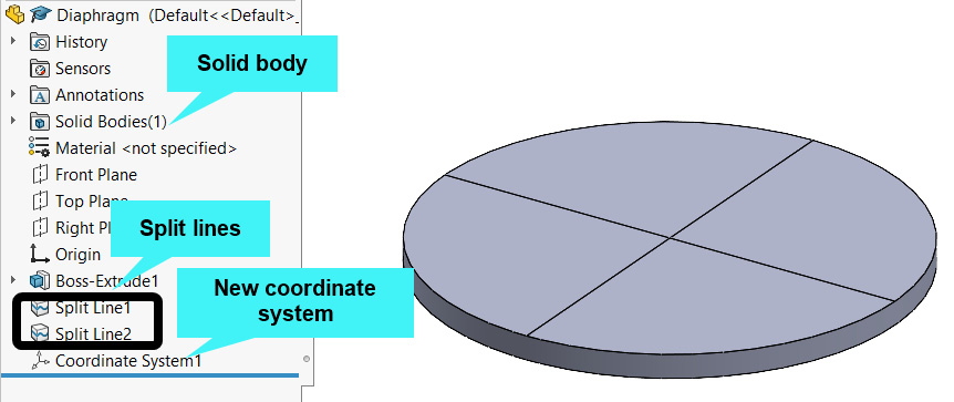
   Figure 9.2 – Reviewing the file of the diaphragm

   From Figure 9.2, you will notice that the model comes with two split lines and one coordinate system. The split lines are needed to facilitate the creation of the new coordinate system. The split line may also be used to examine the variation of radial stress from the center of the diaphragm to the edge.

5. Right-click on Coordinate System1, and then select Edit Feature to expose the Coordinate System property manager, as shown in Figure 9.3.

   Notice that the coordinate's Y-axis goes through the circumference of the diaphragm. We will come back to this in the later section when extracting the diaphragm's stress results:

   

   Figure 9.3 – Examining the axis of the coordinate system

6. Click OK.

This concludes the review, and with the review out of the way, it is time to launch the study.

Dealing with the thermal study

Analyses that involve heat transfer, which is mostly driven by temperature change, are classified broadly under the name thermal study or thermal analyses. Thermal analysis has a unique set of vocabulary and it is a broad topic, with dedicated books covering various aspects of its theoretical foundations [2].

In the context of SOLIDWORKS Simulation, the thermal study environment can be used to investigate the following:

• Transient thermal analyses, where the heat transfer process involves rapid changes with time
• Steady-state thermal analyses, under which the parameters of the heat transfer process do not change rapidly with time

With any of these two types of thermal analysis, the key degree of freedom is the temperature (which is analogous to displacement in static analysis). Moreover, for general thermal analysis, the most important properties of the material needed for the simulation are thermal expansion coefficient, thermal conductivity, and specific heat capacity. Materials within SOLIDWORKS's database without these properties cannot be used for thermal analysis unless you add the properties manually.

In what follows, we shall restrict our focus on a steady-state analysis that involves prescribed temperature states.

Creating the thermal study

With this being the first time dealing with a thermal study in this book, it is good to point out that the purpose of this subsection is to factor in the thermal load caused by the temperature difference on the faces of the diaphragm.

Follow these steps to activate the simulation add-in and launch the thermal study:

1. On the Command manager tab, click on SOLIDWORKS Add-Ins, and then click on SOLIDWORKS Simulation to activate the Simulation tab.
2. With the Simulation tab active, create a new study by clicking on New Study.
3. Input a study name within the Name box, for example, Diaphragm Analysis.
4. Under Advanced Simulation, select the Thermal analysis option, as shown in Figure 9.4:
   

   Figure 9.4 – Launching the thermal study

5. Click OK.

Now that we have launched the thermal simulation study, we can begin to work with the simulation settings.

Selecting thermal options, assigning material, and specifying temperatures

Here, we are going to specify all the requirements for the thermal analysis. Primarily, we shall define the material for the diaphragm, appropriately assign the right temperature values to its top and bottom faces, and run the analysis. The steps to do this are outlined next:

1. To specify the thermal analysis option, right-click on the analysis name and select Properties, as shown in Figure 9.5a. This will launch the thermal study dialog box shown in Figure 9.5b:
   

   Figure 9.5 – Specifying the thermal study option

2. Under the Options tab of the thermal study dialog box, ensure the Steady state type is selected, as shown in Figure 9.5b. This option is consistent with the fact that the temperatures of the surfaces are assumed to remain constant over time.
3. Click OK to close the material database.
4. Back in the simulation study tree, right-click on the part's name (Diaphragm) and choose Apply/Edit Material (Figure 9.6a):
   

   Figure 9.6 – Assigning material to the diaphragm

5. From the materials database that appears, expand the Steel folder, and then assign Chrome Stainless Steel (as indicated in Figure 9.6b).
6. Click Apply and and click Close to close the material database.

   Steps 1–6 complete the specification of the study option and the assignment of material for the thermal study. We will now move on to the specification of temperature.

7. Right-click on Thermal Loads and select Temperature…, as shown in Figure 9.7:
   

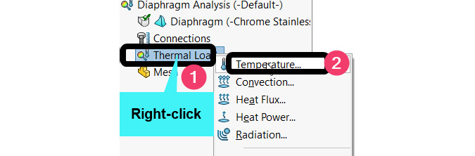
   Figure 9.7 – Initiating the application of temperature load

   Within the Temperature property manager that appears, execute the following actions.

8. Click inside the reference box (labeled 1 in Figure 9.8) and navigate to the graphics window to select the top face of the circular plate diaphragm.
9. Ensure the unit of temperature is Celsius (labeled 2 in Figure 9.8).
10. Specify a temperature of 24.85 (labeled 3 in Figure 9.8):
    

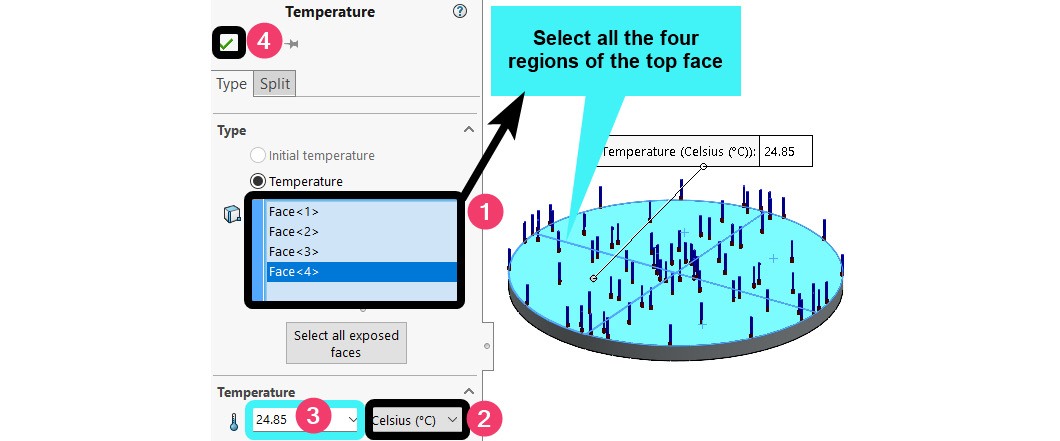
    Figure 9.8 – Specifying the temperature for the top face

11. Repeat step 7, and then follow Figure 9.9 to apply a temperature of 54.85 to the bottom of the circular plate diaphragm:
    

    Figure 9.9 – Specifying temperature for the bottom face

12. Mesh and run the thermal analysis by using the Mesh and Run command, as shown in Figure 9.10:

Figure 9.10 – Meshing and running of the thermal analysis

Once the meshing and running operation is complete, the graphics window will display the thermal plot, as shown in Figure 9.11. As you can see from Figure 9.11, there is only one default result named Thermal1 in the Results folder (unlike in static simulations where three default results are generated after the successful running of a study). This result corresponds to the temperature plot shown in the graphics window. Note how the heat permeates from the bottom to the top side of the diaphragm. Additionally, you will observe that the maximum and minimum temperatures depicted in Figure 9.11 agree with the temperatures we specified for the bottom and top faces of the diaphragm in steps 10 and 11 respectively. This agreement is to be expected since we are dealing with a basic steady-state thermal analysis, with prescribed temperature loads and no consideration of convective heat loss:

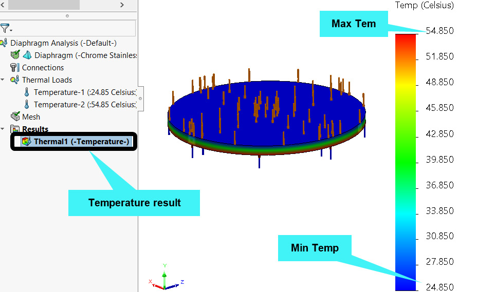
Figure 9.11 – Temperature distribution due to thermal loads on the top and bottom faces

Although we've dealt with a temperature load for this analysis, more complex thermal analyses may involve the application of thermal boundary and forcing functions in the form of heat flux, heat power, convection, and radiation transfer processes (see the options below Temperature… in Figure 9.7). If you want to dig deep into these other options, a good starting point is a book by Kurowski [3].

This concludes the thermal analysis. To reiterate, with the activities carried out in this subsection, we have delved into a steady-state thermal analysis through which we have applied temperatures on the faces of the diaphragm. Technically, what follows from the exposure of the bottom face of the diaphragm to the high temperature is radial expansion. In the next section, we will see how this expansion plays out when the diaphragm is constrained on the edge during the static study.

Dealing with the combined thermal static study

Part of our objective with the static study to be conducted here is to apply external pressure on the surface of the diaphragm so that its maximum deflection can be quantified under a proper constrain. But in addition to pressure load, we shall also carry over the effect of thermal analysis into the static analysis.

Launching the static study

The following steps should be followed to launch the static study:

1. Navigate to the base of the graphics window, right-click on the Study tab, and then select Create New Simulation Study, as shown in Figure 9.12a.
2. Within the Study property manager that pops up, provide a name for the new study, for example, Diaphragm Static, as shown in Figure 9.12b.
3. Select the Static option, as shown in Figure 9.12b.
4. Click OK.

Figure 9.12 – (a) Initiating a new static study and (b) naming the new study

Once steps 1–4 are completed, a new study tab for the static study will be created beside the thermal study tab at the bottom of the graphics window. With this done, our next focus is to integrate the thermal results with the static study (this is the salient feature of this case study).

Integration of thermal results with static study

In contrast to our previous foray into the static study, we need to incorporate the temperature distribution from the thermal analysis into the static study. To achieve this, follow these steps:

1. Ensure you are within the newly created static study, as shown in Figure 9.13. While within the static study window, also take note of the status of the external load (currently empty):
   

   Figure 9.13 – Examining the new static study

2. Right-click on the analysis name, and then select Properties (as we did in Figure 9.5a).

   The preceding step initiates the static study dialog box within which we now need to make the following changes.

3. Navigate to the Flow/Thermal Effects tab, as shown in Figure 9.14.
4. Under Thermal options, tick inside Temperatures from thermal study (labeled 1 in Figure 9.14). This step will link the thermal results from the Dealing with the thermal study section with the current static study:
   

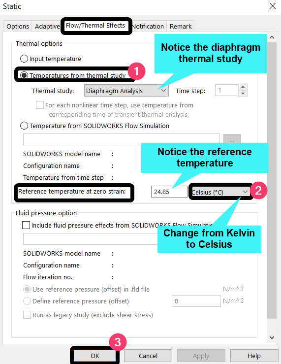
   Figure 9.14 – Modifying the static study dialog box to include the thermal effect

5. In the box labeled 2, change the unit of temperature from Kelvin (K) to Celsius (oC).

   Take note of the number 24.85, which indicates the Reference temperature at zero strain value.

6. Click OK.

The completion of steps 1–6 introduces a new item called Thermal under External Loads, as displayed in Figure 9.15:

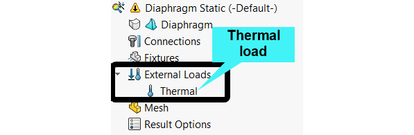
Figure 9.15 – Evidence of a linked thermal load for the static study

A Remark on a Common Error in Thermal Stress Analysis

You may have noticed that the value of the reference temperature at zero strain (which is 24.85oC) that was highlighted in step 5 of this subsection matches the value of the temperature we applied in step 9 of the Selecting thermal options, assigning material, and specifying temperatures subsection. This value (24.85oC) is considered to be the ambient temperature at which material properties such as Young's modulus and Poisson's ratio are obtained during experimental testing. Consequently, it means that the top face of the diaphragm is assumed to be at ambient temperature, while its bottom face, which is exposed to a temperature of 54.85oC, amounts to a difference of 30oC. One of the common mistakes by beginners, using SOLIDWORKS and other finite element software, is to unwittingly consider the ambient temperature to be 0oC. If we had done that, a temperature difference of 54.85oC would have resulted.

After coupling the thermal effect with the static study, we are primed to deal with the other items in the static study.

Applying materials, fixtures, pressure, and runs

This section assumes you have already gone through the past chapters. This means you should be already familiar with how to assign material property, apply fixtures, apply external loads, and create a mesh and run the analysis. For this reason, the condensed steps to deal with the aforementioned items are summarized as follows:

1. For the material, assign Chrome Stainless Steel.
2. For the boundary application, apply a Fixed Geometry fixture, as shown in (a) in Figure 9.16.
3. For the load, apply an external pressure of 0.5 MPa to the top of the diaphragm, as shown in (b) in Figure 9.16:
   

   Figure 9.16 – Applications of fixed support and external pressure

4. Discretize the structure with a fine mesh via the curvature-based meshing algorithm, as shown in Figure 9.17a. The final meshed structure is depicted in Figure 9.17b:

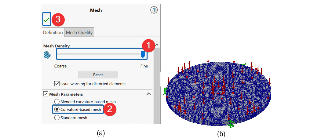
Figure 9.17 – (a) Creating a curvature-based meshing and (b) the meshed body

We are now set to run the analysis and obtain the results.

Running and examination of results

Our goal here is to obtain and compare the results of the static analysis with and without the thermal effect. For this purpose, follow these steps:

1. Run the analysis in the usual manner by following Figure 9.18:
   

   Figure 9.18 – Running the static study with the linked thermal load

   With the running completed, the three default results of Stress1(-vonMises-), Displacement1 (-Res Disp-), and Strain1(-Equivalent-) will appear under the Results folder within the simulation study tree. For design purposes, it is good to track the resultant displacement and the von Mises stress results, both of which are shown in Figure 9.19 and Figure 9.20:

   

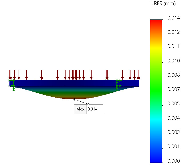
   Figure 9.19 – The resultant displacement of the diaphragm under thermal and mechanical loads

   

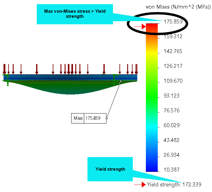
   Figure 9.20 – The distribution of the von Mises stress of the diaphragm under thermal and mechanical loads

   The preceding results amount to the combined effect of mechanical and thermal loads. Figure 9.19 shows that the maximum resultant displacement is 0.014 mm. Meanwhile, in Figure 9.20, you will notice that the von Mises stress surpassed the yield strength of the material, which means the combined effect of the thermal and mechanical loads generates huge stress that will cause the diaphragm to yield. In the subsequent subsection, we will explore how to steer the design away from failure.

   Now, suppose that the diaphragm is subjected to the effect of only the pressure load without the thermal effect – what would be the magnitude of the stress in the diaphragm? To answer this question, we will carry out the next step.

2. Right-click on the analysis name, and then select Properties (as we did in Figure 9.5a).
3. When the static study dialog window appears, navigate to Flow/Thermal Effects, as shown in Figure 9.21, and then select the Input temperature box. This will deactivate the temperature load from the thermal study:
   

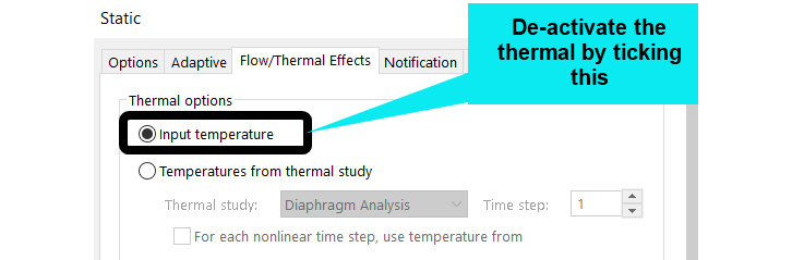
   Figure 9.21 – A partial view of the static study dialog window to uncouple the thermal effect

4. Click OK to close the Static Study PropertyManager.

   As soon as step 4 is completed, a warning symbol will appear beside the analysis name, as shown in Figure 9.22a, and the thermal load will disappear, as shown in Figure 9.22b:

   

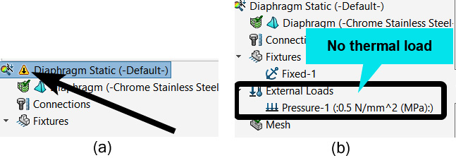
   Figure 9.22 – (a) A warning to rerun the analysis and (b) the absence of a thermal load

5. Rerun the analysis.

   From the results generated, Figure 9.23 (a and b) highlights the displacement and the von Mises stress of the diaphragm due to the pressure load effect alone:

Figure 9.23 – Resultant displacement and the von Mises stress due to the pressure effect alone

From Figure 9.23a, we can see that the vertical displacement of the diaphragm is 0.013 mm when we consider only the pressure effect. This is about 7.7 % less compared to when both thermal and pressure effects were considered. Now, unlike the displacement value, the von Mises stress exhibits experience a much lower value of 34.56 MPa compared to 184.39 MPa when both thermal and pressure effects are considered, which amounts to a difference of 400%! What is the cause of this huge stress?

You will observe that when we conducted the thermal analysis (in the Dealing with the thermal study subsection), we did not apply any fixture to the diaphragm. This means the structure was able to freely expand in all directions. By allowing it to expand freely, no stress will be developed within it. Thus, we have a case of strain without stress. However, within the static study environment, we applied pressure, considered the thermal effect, and constrained the diaphragm by preventing the movement of its edge. By constraining the diaphragm, the normal expansion that would have been caused by the rise in temperature is prevented. This then generates an additional compressive load to be imposed on the diaphragm in addition to the pressure load. So, in short, the higher stress during the combined thermal and static analysis boils down to the interaction between the pressure-induced stress and the internal compressive stress within the diaphragm resisting the temperature-induced expansion.

Recall that while reviewing Figure 9.20 earlier, we mentioned that the huge von Mises stress under the combined thermal plus static study is more than the yield strength of chrome stainless steel, which signals failure. The crucial question we need to answer is how to achieve the goal of designing the diaphragm to be able to handle both the thermal and pressure loads without failing. For this, we shall introduce the concept of optimization study in the next section.

Updating the geometry and rerunning the analysis

Assuming the material selection option is restricted to chrome stainless steel, and we now wish to determine the combination of diameter and thickness that will produce an acceptable stress level within the diaphragm, we may either resort to a crude trial-and-error method (which is akin to searching in the dark while being blindfolded) or adopt a more systematic optimization. To showcase another important capability of SOLIDWORKS Simulation, we will embrace the optimization approach.

We will lay out the procedure for the optimization in the next few pages, so follow along to complete to steps:

1. Include the thermal effect in the static analysis setup and rerun the analysis (see Figure 9.14).
2. At the bottom of the graphics window, right-click the static study tab and select Create New Design Study, as shown in Figure 9.24:
   

   Figure 9.24 – Initiating the New Design Study tab

   The preceding step will launch the optimization design environment with the default look, as shown in Figure 9.25. As you can see from this figure, we need to specify three sets of optimization parameters in the form of Variables, Constraints, and Goals:

   

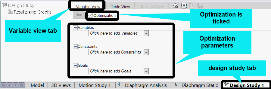
   Figure 9.25 – Optimization study

   Let's briefly take a look at what each of these means:

   1. Variables: This refers to factors within the design that are allowed to change. For many simulation tasks, this often involves geometric features of our design.
   2. Constraints: This represents a condition that our final design should satisfy. For most static analyses, this may involve reducing the deformation, strain, or stress within our design to an acceptable level.
   3. Goals: This generally refers to something we wish to minimize or maximize.

   We will specify these three parameters in the upcoming steps.

3. Under Variables, click on the drop-down menu arrow, and then click on Add Parameter, as shown in Figure 9.26a. This action will launch the Parameters manager that is partially shown in Figure 9.26b:
   

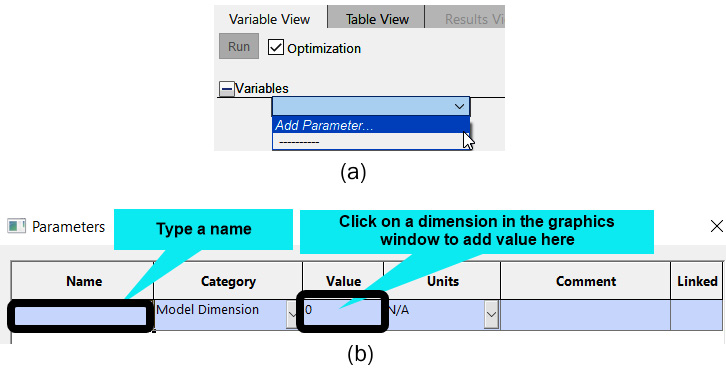
   Figure 9.26 – Adding a parameter under the optimization variable

   Within the Parameters window, our focus will be on the first three columns – Name, Category, and Value.

4. In the column named Category, the Model Dimension option is selected by default, as shown in Figure 9.26b; keep it as such.
5. Now, click inside the box under Value, and then navigate to the graphics window to click on the diameter dimension, as shown in Figure 9.27. This will instantly fill the box with the value of 60, which is the diameter of the diaphragm.
6. Click OK:
   

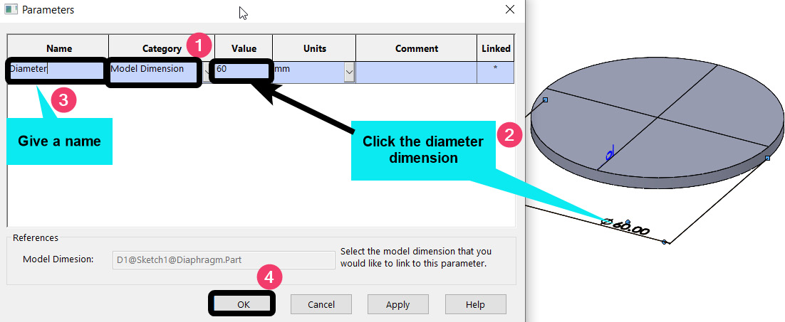
   Figure 9.27 – Adding the diaphragm's diameter as one of the optimization variables

7. Repeat steps 2–5 to add thickness as another parameter, as shown in Figure 9.28, and then click OK to wrap up the selection:
   

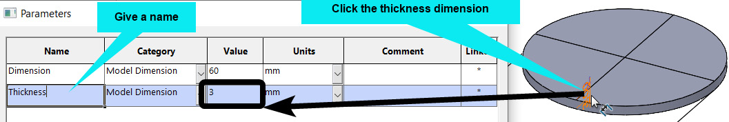
   Figure 9.28 – Adding the diaphragm's thickness as the second optimization variable

8. With step 6 completed, you will be back at the Variable View tab. From here, change the interval boxes for each variable to the Range type and set the upper and lower limits, as shown in Figure 9.29:
   

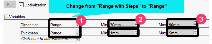
   Figure 9.29 – Updating the variables interval type and ranges

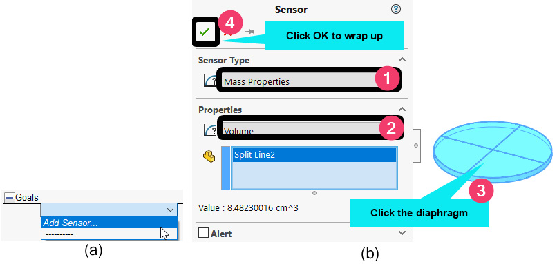
9. Still within the Variable View tab, under Constraints, click on the drop-down menu arrow, and then click on Add Sensor, as shown in Figure 9.30a. This action will launch the constraint's Sensor property manager.
10. Within the Sensor property manager, set the options shown in Figure 9.30b:
    

    Figure 9.30 – Adding and updating the sensor details for the constraint

    By completing step 9, you will be back at the Variable View tab again; make the following changes.

11. Under Constraints, change the sensor type to Is less than and set the Max value to 145 MPa, as indicated in Figure 9.31:
    

    Figure 9.31 – Setting the limit of the von-Mises stress

12. Under Goals, click on the drop-down menu arrow, and then click on Add Sensor, as shown in Figure 9.32a. This action will launch the goal's Sensor property manager.
13. Within the goal's Sensor property manager, set the options shown in Figure 9.32b:
    

    Figure 9.32 – Adding and updating the sensor parameter

14. By completing step 12, you will be returned to the Variable View tab; ensure that the goal option is set to Minimize.

    Once all the three important parameters are set, the Run button will become active, and the interface should look like Figure 9.33:

    

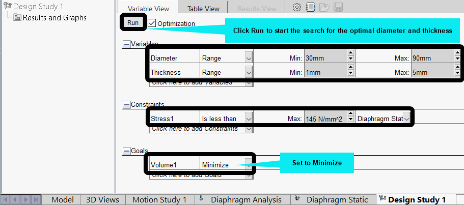
    Figure 9.33 – The complete setup of the optimization study

    A Summary of the Optimization Setup

    Find the combination of diameter and thickness within the specified range specified that will have a minimum volume of material to be used to design the diaphragm, while satisfying the condition of having a von Mises stress that is less than 145 MPa.

15. Click Run to begin the optimization search, which will launch the optimization iteration window shown in Figure 9.34:

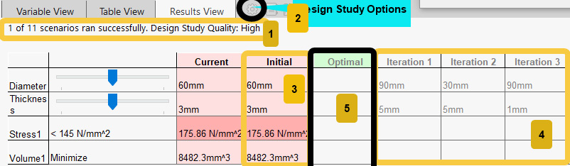
Figure 9.34 – Results View with the iteration window

Let's briefly discuss a few items from Figure 9.34:

• The first is the fact that the optimization iteration involves 11 scenarios, as indicated in the item labeled 1. Still with the item labeled 1, notice that the status of the study option is indicated by the phrase Design Study Quality: High. Typically, High is the default option, but you can set the quality by using the Design Study Options button labeled 2.
• Next, the initial values of the design parameters are indicated in the box labeled 3, while the combinations of various values of diameter and thickness are contained in the partially shown iterations table labeled 4.

  At the end of the optimization run, the optimization algorithm will sort through the iteration to find the set of parameters that fits our design constraint (that is, with a von Mises stress less than 145 MPa) while meeting the goal of minimizing the volume. Once found, the column named Optimal will be filled accordingly. If no optimal solution is found, then you will get an Optimization failed message.

Fortunately, the running of the current study is a success, as shown in Figure 9.35:

Figure 9.35 – Results View with the optimal solution

As you can see from Figure 9.35, within the range of values that we have considered, the optimization result yields an optimal solution that turns out to be a combination of diameter and thickness values of 30.01 mm and 1.68 mm respectively. How does this reduction impact the performance of the diaphragm? For one, this combination yields a von Mises stress of 137.71 MPa, which is 27% lower than the value of 175.86 MPa we started with. Additionally, the von Mises stress we obtained is also very much lower than the yield strength of chrome stainless steel, which means the design is now much safer. Relatedly, you will also see that the new volume of 1190.85 mm3 is lower than the initial volume of 8482 mm3 (see the Optimal and Initial columns in Figure 9.35).

Finally, by clicking on any of the iteration columns, you would make its result active in the graphics environment and the associated study environments. For instance, the Optimal column has been clicked to make it the current study. After making it the current study, you can then switch to the coupled static study environment. Upon switching, you will spot two artifacts of the optimization study, as illustrated by the von Mises stress plot shown in Figure 9.36. The first artifact to note is the presence of the two sensor items (which we created in steps 9 and 12) under the features manager tree (labeled 1). Second, there will be a new item named Parameters (labeled 2) embedded within the simulation study tree:

Figure 9.36 – Examining the updated von Mises stress based on the optimal parameters

You can right-click on the two artifacts highlighted previously for further explorations, and you can examine other results obtained in the case of combined static and thermal study. Meanwhile, for verification purposes, three more results are shown in Figure 9.37, Figure 9.38, and Figure 9.39:

Figure 9.37 – The resultant displacement with the optimal parameters under pressure load alone

Figure 9.38 – The radial stress obtained with the optimal parameters under pressure load alone

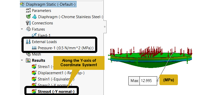
Figure 9.39 – The tangential stress obtained with the optimal parameters under pressure load alone

For the three preceding results, the thermal analysis was deactivated (as done earlier in Figure 9.21) so that only pressure load is used for the analysis (using post-optimization geometric data). Interestingly, these last three results can be compared with the output from the following expressions for the axisymmetric analysis of thin plates [4]:

• ymax (occurs at the center of the plate) = (9 - 1)
• Maximum radial stress = 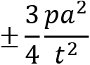(9 - 2)
• Maximum tangential stress = (9 - 3)

In the preceding equations, v and E are material properties denoting the Poisson's ratio and Young's modulus respectively. The a and t parameters symbolize the radius and thickness of the diaphragm, while p is the applied pressure. By substituting the value of v = 0.28, p = 0.5 MPa, E = 200 x 109, t = 1.68 mm, and a = d/2 = 15 mm in the preceding theoretical equations, we obtain the value of 0.0046 mm for the maximum deflection, 29.99 MPa for the radial stress, and 14.95 MPa for the tangential stress. As you can see, the theoretical deflection value differs from the one computed by SOLIDWORKS by just 8.7%, while the stresses differ by 10% and 13% respectively. Take note that the high difference between the values from the theoretical expressions and the simulation results can be attributed to the fact that a collection of solid elements is used for the study (for thin plates, shell elements, covered in Chapter 5, Analyses of Axisymmetric Bodies, give better accuracy).

This concludes the solution to the case study on the exploratory design analysis of a diaphragm under the combined influence of temperature and mechanical loads. Over the last several pages, we have described the procedure for coupling a thermal study with a static study. Along the way, we conveyed the strategy for including and excluding temperature effects in a static study and demonstrated how to employ SOLIDWORKS Simulation's optimization capability to obtain optimal geometric parameters for the problem studied. Moving forward, it is necessary to emphasize that apart from thermal loads, another type of load that is of importance to design engineers is cyclic load, which is the focus of the next section.

Analysis of components under cyclic loads

The effect of cyclic loads is closely related to fatigue failure, which is another broad topic on its own. In the past chapters, we have based the failure assessments of components that we studied on the idea that failure will happen if a specific stress measure exceeds the yield strength (for ductile components) or the ultimate strength (for brittle components). With fatigue failure, the stress required to bring a component to failure is often far lesser than the yield or ultimate strengths of the material under study. According to numerous studies, more than 50% of machinery breakage can be attributed to fatigue failure [4, 5]. While this section is not intended to cover fatigue failure in detail, we will outline four major concepts that you need to be aware of to conduct a basic fatigue analysis:

• Stress-time or load-time cycle: This is the plot of stress/load versus time that describes the cyclical nature of the stress/load applied to a component. Different forms of this curve occur in a variety of practical scenarios. Two common examples shown in Figure 9.40 are as follows:
  1. The fully reversed stress cycle, which is most commonly used for laboratory fatigue tests, and where the maximum and minimum stresses are equal in magnitude but opposite in sign.
  2. The zero-based stress cycle where the minimum stress is zero but the maximum stress is some other positive number:

Figure 9.40 – Two examples of stress cycles

• S-N or the Wöhler curve: This is the curve of stress versus the number of cycles to fracture (that is, when the component breaks apart). Most S-N curves are based on the fully reversed load/stress cycles. For cases of loading in which the stress/load cycle is not fully reversed, empirical fatigue expressions such as Goodman, Soderberg, and Gerber relations must be used to complement the S-N curve.
• Fatigue limit/endurance limit: This refers to the stress level below which a component can undergo an infinite number of stress cycles without failure. It is an important number that is determined by an S-N curve.
• Fatigue life: This is an important outcome of interest in fatigue analysis. It refers to the number of cycles that a component is subjected to under a specific load before fracture takes place. Quite often, fatigue life is affected by many factors, including environmental factors, microstructural flaws in materials, manufacturing-induced defects, the presence of stress raisers, and so on [6].

With this admittedly brief background, let's now examine an example that features these concepts in the context of SOLIDWORKS Simulation.

Problem statement

A thin stepped bar of 10 mm thickness is subjected to a static pressure load of magnitude 200 MPa, as shown in Figure 9.41. The bar is made of alloy steel with a yield strength of 620 MPa and an ultimate strength of 810 MPa. Our objectives with this problem is as follows:

• To conduct a static analysis to determine the stress in the component with a non-cyclical application of the load
• To connect the previous static study with a fatigue analysis of the component under a fully reversed cyclical application of the pressure load to determine its fatigue life and to verify whether or not fatigue failure occurs in the component based on a design life of 106 cycles:

Figure 9.41 – A tensioned steel bar with two stress raisers

The next section addresses the problem.

The solution to fatigue analysis

As with the thermo-mechanical analysis conducted in the previous section, a preliminary static analysis is generally conducted prior to doing a fatigue analysis. To make the presentation concise, a file is presented that contains an implemented static analysis, which is what is reviewed next.

Review of the static study

To begin this exercise, download the file named FilletedBar within the Chapter 9 folder that you downloaded for the previous exercise. Given that you are now fully familiar with the setup for static studies, the file contains both the geometric model and a completed static study:

Let's now review the file:

1. Open the part file (FilletedBar) via File  Open.
2. If the simulation add tab has not been initiated, then activate it via the Command manager tab done as we have been doing.
3. Once the simulation tab is active, you will see the static study tab; rerun the analysis and the simulation items will appear, as shown in Figure 9.42:
   

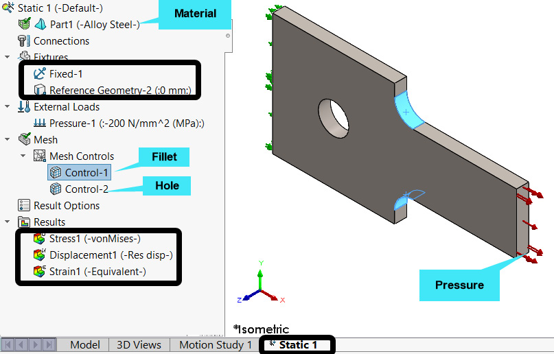
   Figure 9.42 – Examining the implemented static study

4. Double-click on the Stress1 result to visualize the von Mises stress (Figure 9.43):
   

Figure 9.43 – Distribution of the von Mises stress under the static load

Note that the maximum von Mises stress (389.934 MPa) revealed in Figure 9.43 is less than the yield strength of the material (620 MPa). This gives the impression that the component is safe. In the next subsection, we will strive to draw further insight into the safety of the component from a fatigue analysis.

Fatigue analysis

Here, we will check for the possibility of fatigue failure if the component is subjected to a cyclical form of the preceding stress. The procedure for fatigue study comprises the following steps:

1. Navigate to the base of the graphics window, right-click on the study tab, and then select New Simulation Study (as we did in Figure 9.12a).
2. Within the Study property manager that appears, under Advanced Simulation, click Fatigue.
3. Select the Constant amplitude events with defined cycles option (labeled 2 in Figure 9.44).
4. Provide a name for the new study and wrap up by clicking OK, as shown in Figure 9.44:
   

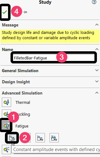
   Figure 9.44 – Initiating the fatigue study environment

5. Within the fatigue study simulation tree items, right-click the study name and choose Properties, as illustrated in Figure 9.45:
   

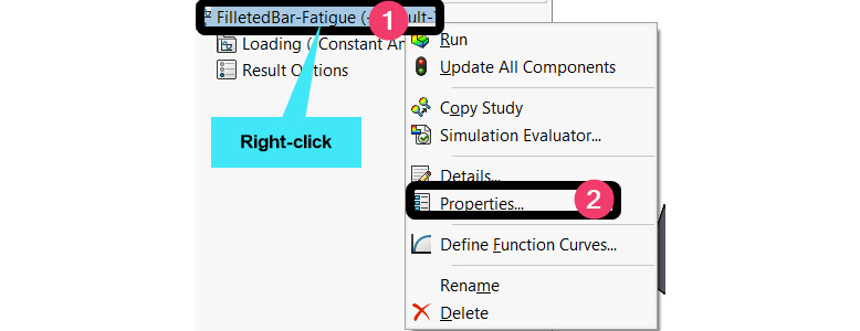
   Figure 9.45 – Modifying the fatigue study property

   This launches the fatigue study dialog box, within which we need to make the following options.

6. Within the Options tab, make the selections shown in Figure 9.46:
   

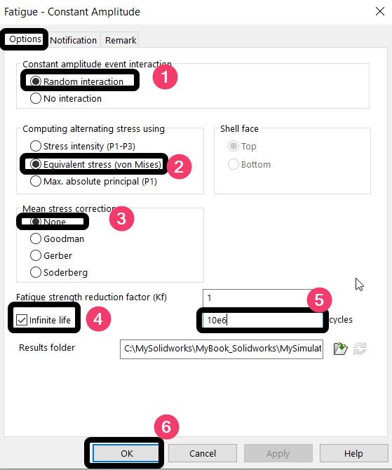
   Figure 9.46 – Fatigue analysis dialog box

   Once you conclude the step by clicking OK, the fatigue study environment will appear. But before we move onto the environment, a couple of comments are desired about the selections in Figure 9.46.

   Note that we have four options under the Mean stress correction item (labeled 3). The first option is most appropriate for a fully reversed stress cycle (such as Figure 9.40a). For a fully reversed stress cycle, the mean stress is zero, and hence there is no need for a mean stress correction factor. However, the other three options, which we also mentioned in the introduction to this section, are used for non-fully reversed stress cycles (such as Figure 9.40b). Among these other options, the most conservative and thus preferable for non-fully reversed stress cycles is the Goodman correction factor. Next, in the box labeled 5, we have chosen the upper limit of 1,000,000 cycles for the fatigue life (N). This number is used because the fatigue strength of most materials is often is specified at N > 106. Furthermore, close to the box labeled 5, note that we maintained the value of 1 for the fatigue reduction factor. For other practical situations, a value less than 1 but greater than 0 may be used to quantify the reduction in the fatigue strength of the component due to the presence of the fillets for instance. Let's now complete the other simulation tree items.

7. Under the fatigue simulation study tree, right-click Loading and choose Add Event as shown in Figure 9.47a.
8. Within the Add Event property manager that appears, follow the screenshot shown in Figure 9.47b:
   

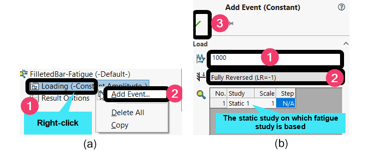
   Figure 9.47 – Specifying the fatigue load parameters

   By completing step 8, a new item will appear within the simulation study tree bearing the name of the model – in this case, FilletedBar.

9. Right-click on the FilletedBar item that appears, and then click Apply/Edit Fatigue Data (Figure 9.48):
   

   Figure 9.48 – Initiating the application of material property

10. Within the material database, follow the selections depicted in Figure 9.49:
    

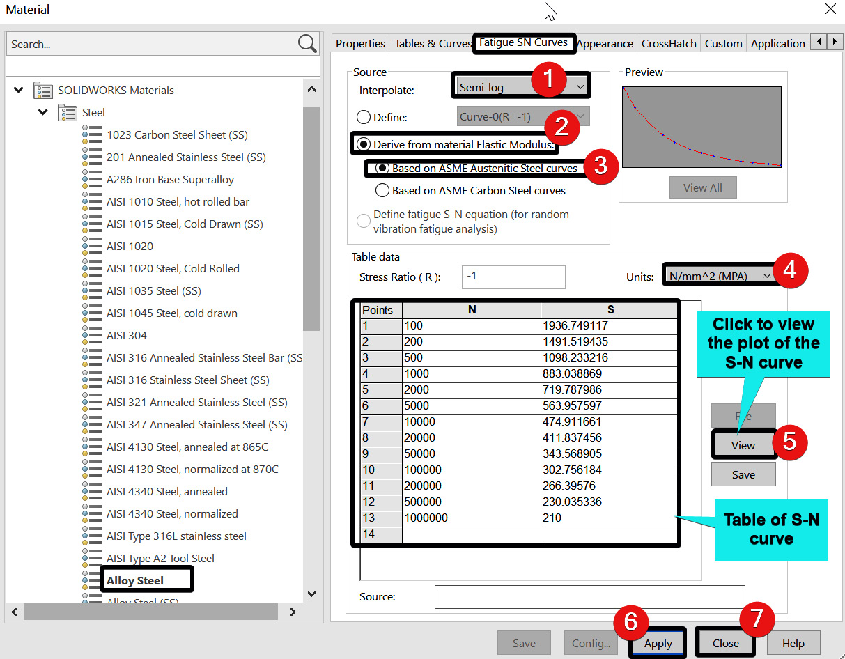
    Figure 9.49 – Material database

    At the center of Figure 9.49 is the table of the S-N curve, which was among the concepts discussed in the introduction to this section. A specific row of the N column represents the number of cycles at which the corresponding stress value in the S column can be applied before fatigue failure. As you can see, the last row of the table indicates that S = 210 MPa is the stress that corresponds to N = 106. This means that the fatigue strength of this material is 210 MPa. So, all things being equal, components derived from this material can be subjected to an infinite cycle of load at stress values that equal or fall below 210 MPa without fatigue failure. There's one more thing – by default, the plot of the S-N plot shown in the top right corner is displayed as a log-log plot. However, it is generally easier to work out the stress that corresponds to the infinite life of the material by changing to the Semi-log option, as done in the box labeled 1. For a better view of the S-N curve, you can click on the button labeled 5, which will create a new window of the S-N curve, through which you can observe that the curve becomes horizontal at S = 210 MPa.

    At this stage, we are done with the setup for fatigue analysis, and we are ready to run the analysis.

11. Run the analysis, as shown in Figure 9.50:

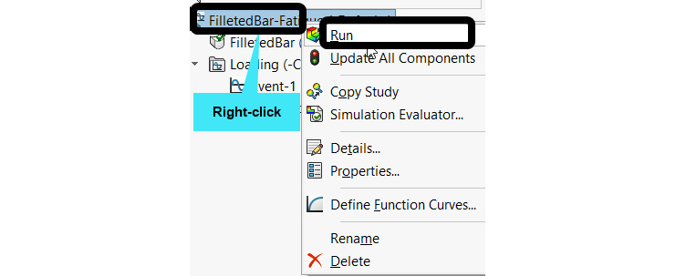
Figure 9.50 – The running of the fatigue study

Once the running is complete, you will notice Results1 (-Damage-) and Results2 (-Life-) under the Results folder. By double-clicking on each, you can reveal the plot of the distribution of the fatigue damage (Figure 9.51) and fatigue life (Figure 9.52):

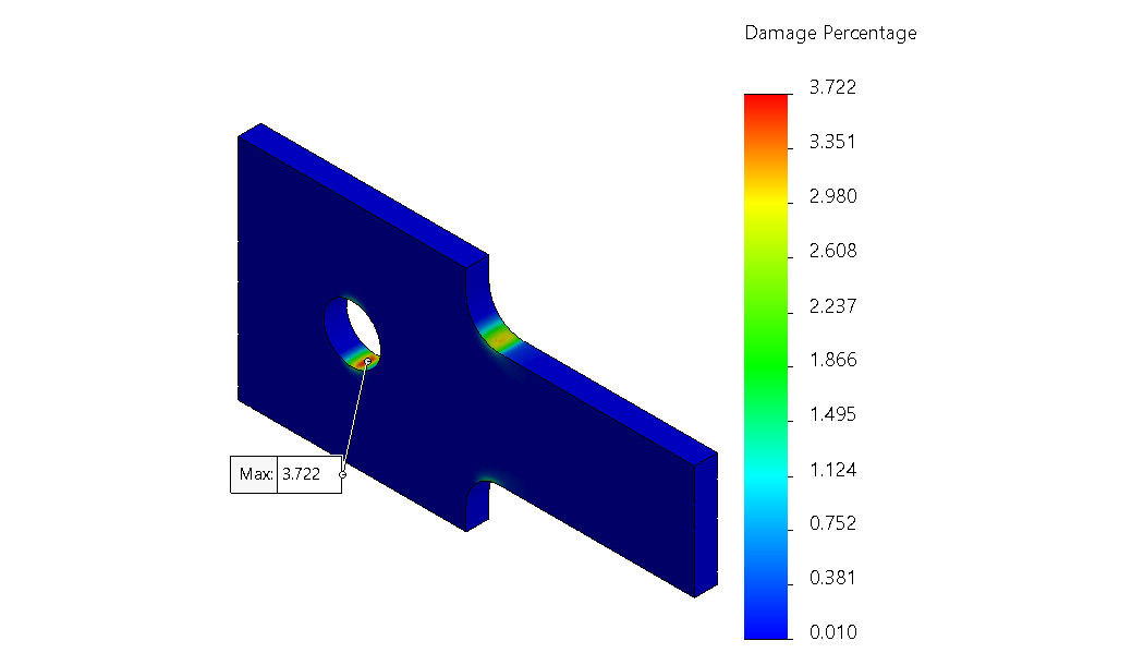
Figure 9.51 – Assessments of fatigue damage

Referring to Figure 9.51 and Figure 9.52, it is obvious that the stress hot spots are located at the fillets and the top and bottom of the hole. This is the same area that the static result revealed in Figure 9.43. However, while the static result gave an impression of safety, Figure 9.52 shows that the fatigue capacity of the component around the hole is significantly less, with a life of 26,828 for a load block of 1,000 (see Figure 9.47b for the load block). According to the literature on the theory of machine design [6], this component will be categorized as having a finite fatigue life, given that it has a region with fatigue capacity in the 103 < N < 106 range.

Finally, the trend of the results in Figure 9.51 and Figure 9.52 is consistent with well-established observations that fatigue failure is naturally initiated by discontinuities in the form of a rapid change in cross section (such as the filleted region and the hole located within the studied component) [6]. Under a repeated cyclical load, discontinuities represent fertile ground for the initiation and propagation of cracks that are closely linked with the fatigue failure mechanism. The good news is that the power of finite element simulation can always be leveraged to investigate the effect of discontinuity such as fillets, keyways, and grooves, as we've done here. However, other critical factors, such as environmental influences in the form of corrosion, surface defects, fabrication flaws, and microscopic defects/inclusions, cannot be easily captured without resorting to advanced fatigue/fracture simulation platforms such as NASGRO, developed by NASA [7]:

Figure 9.52 – A plot of the fatigue life

This ends our exploration of the solution to the problem posed at the beginning of this section. Overall, this last example serves only to give an introductory coverage of the fatigue analysis of a component under the effect of a cyclical load using SOLIDWORKS Simulation. Understandably, we have only looked at a constant amplitude stress cycle premised on a static load. However, SOLIDWORKS Simulation is also capable of dealing with variable amplitude stress cycles premised on a static load. Moreover, it is capable of handling constant/variable amplitude stress cycles based on dynamic vibration loads and analyses, based on more than one static or dynamic study. In all, fatigue analysis is a very delicate and daunting task for most design engineers. Nevertheless, it is hoped that this introduction guides you toward taking a journey to discover other advanced features of this aspect of the simulation environment for more complex analysis.

Summary

This chapter covered the procedures needed to factor in thermal and repeated load cycle effects in the analysis of engineering components, using two hands-on examples. In addressing the problems framed around the examples, we showcased the following strategies:

• How to integrate thermal and static analyses to address the simulation of components at an elevated temperature
• How to investigate the fatigue life for components under the effect of cyclical loads
• How to reap the benefit of the optimization capability of SOLIDWORKS Simulation to design components against failure

These concepts add to your repertoire of analysis techniques, which can be leveraged for a comprehensive assessment of a wide variety of design problems that you are likely to encounter.

In the next chapter, we will round up our coverage of the topics by re-examining certain aspects of meshing that will further solidify your exposure to finite element simulation.

Further reading

• [1] Pressure sensors: The design engineer's guide, AVNET https://www.avnet.com/wps/portal/abacus/solutions/technologies/sensors/pressure-sensors/ (accessed 20/08/2021)
• [2] Design for Thermal Stresses, R. F. Barron and B. R. Barron, Wiley, 2011
• [3] Thermal Analysis with SOLIDWORKS Simulation 2019 and Flow Simulation 2019, P. Kurowski, SDC Publications, 2019
• [4] Advanced Mechanics of Materials, A. P. Boresi, R. J. Schmidt, and Knovel, Wiley, 2003
• [5] Advanced Mechanics of Materials, R. D. Cook and W. C. Young, Prentice Hall, 1999
• [6] Shigley's Mechanical Engineering Design, R. Budynas and K. Nisbett, McGraw Hill Education, 2010
• [7] NASGRO, NASA/Southwest Research Institute https://www.swri.org/nasgro-software-overview (accessed 20/08/2021)