Chapter 8: Simulation of Components with Composite Materials

So far in this book, the simulation examples presented have involved components constructed of isotropic materials – that is, materials for which the properties such as Young's and shear moduli and Poisson's ratio are constant in all directions. However, given that there has been an increase in the use of composite materials in many industries in recent years, knowledge of simulation with these materials has become central to the design of advanced engineering products. For this reason, this chapter taps into SOLIDWORKS's simulation capability for the structural analysis of components made of composite materials. The chapter covers the following topics:

• An overview of the analysis of composite structures
• An analysis of composite beams
• An analysis of advanced composite structures

Technical requirements

You will need to have access to the SOLIDWORKS software with a SOLIDWORKS Simulation license.

You can find the sample file of the model required for this chapter here:

https://github.com/PacktPublishing/Practical-Finite-Element-Simulations-with-SOLIDWORKS-2022/tree/main/Chapter08

An overview of the analysis of composite structures

Before we go into the case study for this chapter, it helps to have some background knowledge about composite materials. Engineering materials such as metals, ceramics, and polymers/elastomers are isotropic by nature. Although each of these families of materials is widely used in their natural isotropic form for many applications, each has its pros and cons. For instance, solid metals (as opposed to liquid metals such as gallium and mercury) are endowed with high stiffness and have high deformability, but are heavy and prone to fatigue failure. Ceramics also have high stiffness, but they are brittle. On the other hand, polymers/elastomers have good corrosion and wear-resistance properties, but they have very low stiffness and temperature-dependent properties. Put together, this indicates that no single class of material is superior under all possible desirable functional working conditions [1] (see the Further reading section at the end of the chapter). In response to the weaknesses of each material family as outlined, research into composite materials has become a key driver of many engineering innovations in recent years.

In the most basic form, a composite is formed when two or more different materials are combined. This combination may involve microscopic or macroscopic combinations. Further, the combination may occur naturally (for instance, wood and bone natural composites) or be artificially engineered. Our interest in this chapter is those that involve artificially engineered macroscopic material combinations. The applications of this class of artificially engineered composite materials can be found in space/aircraft structures, automotive systems, bicycle frames, golf club shafts, energy systems such as wind turbines, and so on. Figure 8.1 illustrates some practical and modern usage of composite materials:

Figure 8.1 – An illustration of the usage of composites [2, 3]: (a) for aircraft bodies, (b) a carbon fiber-reinforced composite wheel, and (c) a cross section of a composite wind turbine blade

Notably, there are also various kinds of artificially engineered composite materials, as depicted in Figure 8.2. A detailed discussion of the difference in the constituent, behavior, properties, and manufacturing of each category in Figure 8.2 can be found in the book by Hyer and White [4]:

Figure 8.2 – Some major categories of composites

As you will see in sections ahead, much of this chapter centers on the analysis of components designed with laminated composites formed from fiber-reinforced composites. In laminated composites, the laminate is formed by stacked layers, with each layer being referred to as a ply (see Figure 8.3a). In turn, each ply is manufactured by reinforcing a matrix (a polymer or metallic material) with fibers (dispersed or oriented). For an illustrative purpose, Figure 8.3b and Figure 8.3c depict two plies with 00 and 900 fiber orientations used to form the stacked laminate in Figure 8.3a. Note that, oftentimes, for better performances, the fibers may be arranged based on other angles of interest. Typically, this angle is with respect to the principal material direction, which is the X axis for the laminates shown:

Figure 8.3 – (a) A laminate formed by stacking of two plies, (b) a ply reinforced with fibers arranged parallel to the principal material direction, and (c) a ply reinforced with fibers arranged transversely to the principal material direction

Now, because of the reinforcement with fibers, a single ply may turn out to have either anisotropic or orthotropic material properties. This means their mechanical properties differ along the three X, Y, and Z directions (for anisotropic material) or the variation is restricted to two of the directions for orthotropic. Some important consequences of this anisotropic/orthotropic material behavior are (i) non-uniform distribution of stress across the laminate's thickness, (ii) development of shear stress between the plies – interlaminar shear stress, and (iii) non-suitability of the simple failure theories we have used in the past chapters for the analysis of these materials.

With the background provided, we shall take on a case study to demonstrate the use of SOLIDWORKS Simulation to analyze the response of an engineering component designed with composite material properties.

An analysis of composite beams

This section details our first case study, which is related to the analysis of a curved composite beam acting as an elastic spring.

Through this case study, you will also become familiar with how to create a custom orthotropic composite material and assign its properties to a collection of composite plies. Furthermore, you will become familiar with the effect of fiber orientations on the behavior of composite structures. Moreover, you will learn the difference between the types of stress available for analysis with composite materials and the type of failure criteria used to estimate their factor of safety. Also covered briefly is the procedure to modify SOLIDWORKS Simulation global settings.

Let's get started.

Problem statement

Figure 8.4a shows a multipurpose prosthetic designed with a fiber-reinforced composite [5]. The structural component of the prosthetic consists of two major segments, BA and AC, as highlighted in Figure 8.4a. Our focus is on the AB segment (isolated in Figure 8.4b) with a thickness of 8 mm and a width of 120 mm. This segment is formed by a curved beam and acts functionally as an elastic spring:

Figure 8.4 – (a) A multi-purpose prosthetic fitness foot by Ottobockus [5], (b) the solid model of the upper elastic spring, (c) a laminate with fiber orientations [0/902/45/45/902/0], and (d) a laminate with ply orientation [0/-45/45/90/90/45/-45/0]

The goal of the simulation is to investigate the static performance of the BA segment if it were to be designed with a laminate made of Carbon Fiber-Reinforced Polymer (CFRP) composites under the combinations of ply orientations shown in Figure 8.4c and Figure 8.4d. The orthotropic material properties of the CFRP are listed in Table 8.1. To be more specific, we want to answer the following questions about the orientations:

• What is the maximum resultant displacement of the elastic spring?
• What is the maximum normal stress across all the plies?
• What is the minimum factor of safety of the structure?

A load of 100 N is assumed to be applied on a small area around point B in Figure 8.4 of the elastic spring. This area is shown later in Figure 8.5:

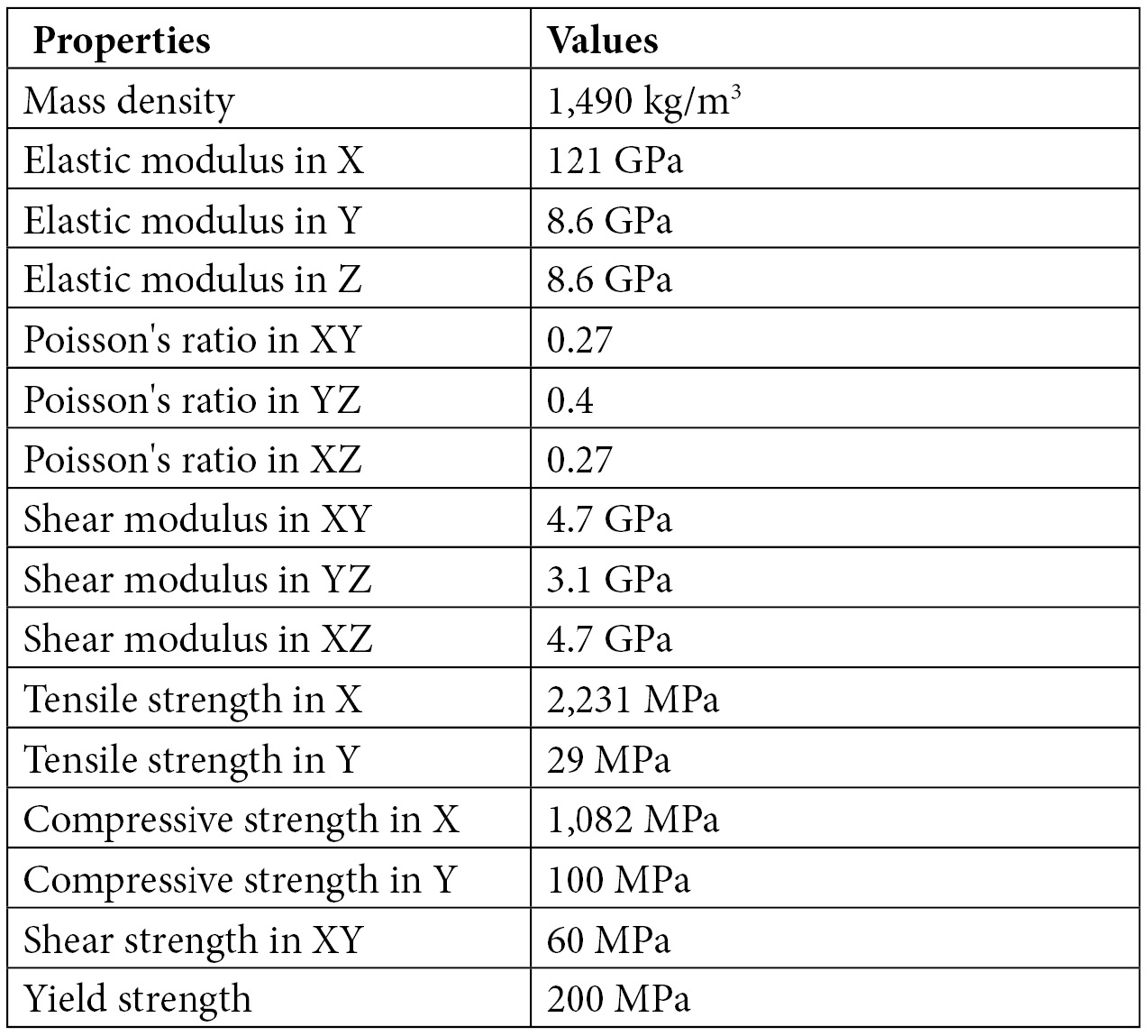
Table 8.1 – The elastic orthotropic properties of CFRP

As you can see from Table 8.1, as opposed to the materials we have seen in all previous chapters, the key mechanical properties for the static analysis of the CFRP composite are specified along the X, Y, and Z directions.

Note on Laminate Nomenclature

In the caption for Figure 8.4c, we specified the set of angles for the laminate as [0/902/45/45/902/0]. Note that 902 is shorthand for two repetitions of 90. Another shorthand is also commonly used in a composite description when the laminate has symmetric plies. For instance, the two laminates in Figure 8.4c and Figure 8.4c are symmetric about the midplane. Owing to this, we could have written [0/902/45/45/902/0] as [0/90/90/45]s, where the s subscript denotes that we have four more plies with a set of angles that mirror the four spelled out, which is [45/90/90/0]. In the same spirit, we could also have written [0/-45/45/90]s for the laminate in the caption for Figure 8.4d. You will see the symmetric notation later in this chapter.

In pursuit of the solution to the problem, we shall now go through a series of steps in the upcoming sections to answer the questions attached to the problem statement.

Part A – reviewing the structural model

To get on track with the simulation study, we will first review the model and then activate the simulation study in this section.

Reviewing the file of the curved elastic spring

To get started, download the Chapter 8 folder from this book's website to retrieve the model of the curved beam. After downloading the folder, follow these steps:

1. You should check to see that it comprises a SOLIDWORKS part file named Prosthetics_ElasticSpring.
2. Extract the file and save it on your PC/laptop.

   Let's now briefly go over some of the features of this file. To begin with, you need to get into the SOLIDWORKS environment.

3. Start up SOLIDWORKS.
4. Select File  Open, and then open the part file named Prosthetics_ElasticSpring.
5. Navigate to the Feature Manager design tree and examine the details, as shown in Figure 8.5:

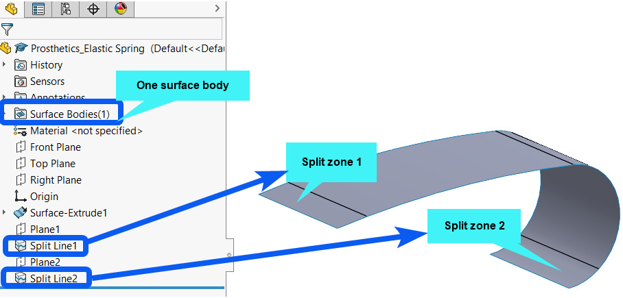
Figure 8.5 – Reviewing the file of the structure

The first thing you will probably notice from Figure 8.5 is that we have 1 surface body created using the Surface Extrude tool. In effect, this surface body represents the surface equivalent of the BA segment in Figure 8.4b.

From this, we need to get an important lesson out of the way – to analyze a composite part within the SOLIDWORKS Simulation environment, you can only employ a surface body (a weldment and solid extruded body are not allowed).

The other thing you will observe is that there are two split lines (Split Line1 and Split Line2). The split lines are created so that we have separate regions for the application of the load (on zone one) and the application of the boundary condition (on zone two).

Activating the simulation tab and creating a new study

With the key features of the file reviewed, you can go ahead and launch the simulation study as we normally do, as highlighted next:

1. Under the Command manager tab, click on SOLIDWORKS Add-Ins, and then click on SOLIDWORKS Simulation to activate the Simulation tab.
2. With the simulation tab active, create a new study by clicking on New Study.
3. Input a study name within the Name box, for example, Prosthetics_ElasticSpring Analysis.
4. Keep the Static analysis option, and then click OK.

Now that we have activated the simulation study, we can begin to work with the items in the Simulation study tree, which, as shown in Figure 8.6, indicates that we need to define the thickness for the surface body:

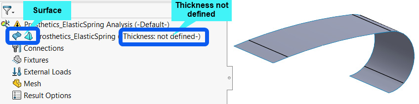
Figure 8.6 – Examining the surface body within the simulation study tree

The next section will walk you through the crucial procedure to convert the surface body into a composite shell. It further discusses some key concepts around the creation of orthotropic composite plies.

Part B – defining the laminated composite shell properties

This section is devoted to the procedure for defining and scrutinizing the properties of the composite plies used in the build-up of the laminated composite shell. It also includes brief subsections on the specification of the fixture and external load on the structure.

Let's begin with the composite material details.

Defining the properties of a multilayered composite shell

The surface body we examined in the previous section will form the basis of the composite shell. In what follows, we shall go through a somewhat long but important series of steps to define the properties of the laminated composite shell.

Carefully follow along:

1. Within the simulation study tree, right-click on the surface body, and then select Edit Definition, as shown in Figure 8.7:
   

   Figure 8.7 – Initiating the thickness definition for the surface body

   With this, the Shell Definition property manager will pop up, as shown in Figure 8.8. This is a familiar window that you will have seen in past chapters. However, we shall not be using the Thin option as in all our previous encounters with this window:

   

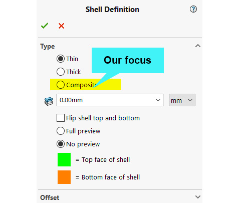
   Figure 8.8 – Shell Definition property manager

2. Within the Shell Definition property manager, under the Type option, select Composite, as shown in Figure 8.8. The selection of the Composite option here immediately opens up access to the Composite Options section in the lower region of the manager. It also creates and attaches a separate coordinate system to the shell structure, as shown in Figure 8.9:
   

   Figure 8.9 – Shell Definition property manager with the Composite option

   Note that the gray arrow in the composite coordinate system, which is attached to the shell in the graphics window, always aligns with the ply angle. In other words, it represents the local fiber orientation. Thee items that we shall work with have also been annotated, that is, Total Plies, Thickness/Angle box, and the Material box. We shall now carry out some further steps with these items.

3. In the Total Plies value box (labeled 1 in Figure 8.10), key in 8:
   

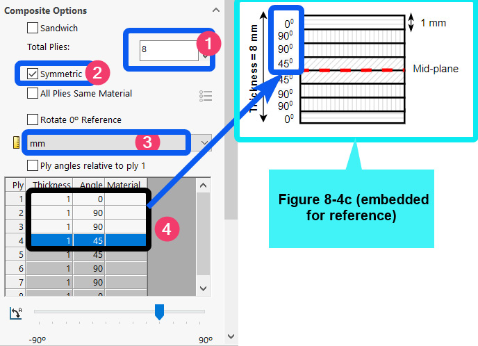
   Figure 8.10 – Specifying the ply number, thickness, and angle

4. Tick inside the box labeled 2 (Symmetric) and ensure the unit is in mm (as indicated in the box labeled 3 in Figure 8.10).
5. In the ply property specification box, labeled 4 in Figure 8.10, key in, one by one, the four respective values of thickness (1, 1, 1, and 1) and angles (0, 90, 90, and 45).

   Note that the values we have keyed in belong to the top half of the composite laminate shown in Figure 8.4c. Furthermore, because the laminate is symmetric and we've ticked Symmetric in step 4, SOLIDWORKS automatically completes the last four rows in the grayed-out area. It goes without saying that if the ply combination is not symmetric, then we have to add the values of thickness/angle for all plies ourselves.

   Now, you will notice that the Material column in the box labeled 4 in Figure 8.10 is empty. Our next task is to define this.

6. To define the material property for the plies, tick inside All Plies Same Material, and then click the box labeled 2 in Figure 8.11. Doing this will activate the material database:
   

   Figure 8.11 – Material specification

7. Within the material database, navigate to the folder named Custom Materials, right-click, and then click on New Category (Figure 8.12a). With this, a new material folder will be created with a default name of New Category.
8. Change the name to MyComposite (Figure 8.12b):
   

   Figure 8.12 – Creating a new composite material category under the Custom Materials folder

9. Right-click on the MyComposite folder and click on New Material, as shown in Figure 8.13a. With this step, a new material file will be created with a default name of Default; modify the name to CustomCFRP, as shown in Figure 8.13b:
   

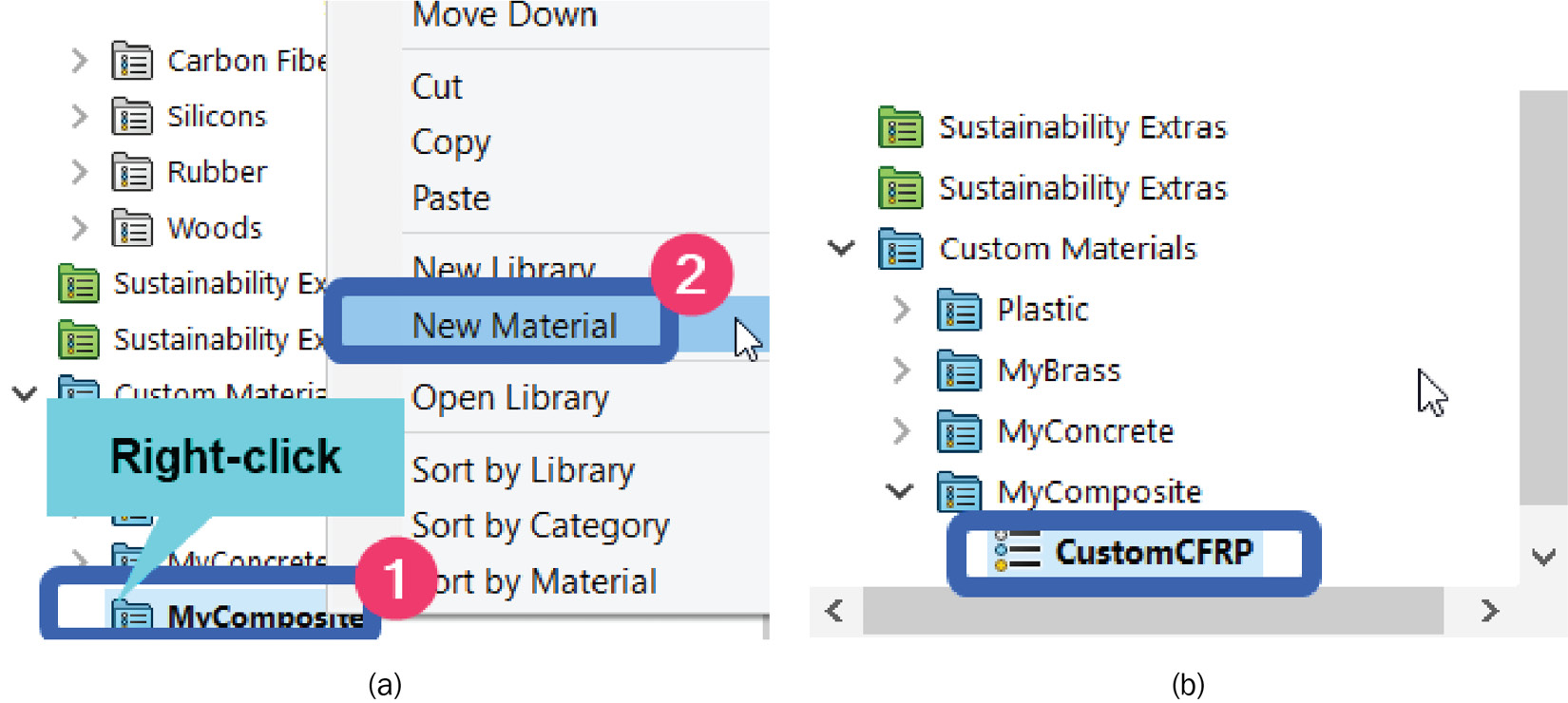
   Figure 8.13 – Creating the CFRP material file

   We shall now work on the right side of the material database to define the properties.

10. On the right side of the material database, under Model Type, select Linear Elastic Orthotropic (labeled 2 in Figure 8.14). This is very important. The default is Linear Elastic Isotropic. Thus, you need to make sure Linear Elastic Orthotropic is chosen.
11. Ensure the unit remains as SI – N/m^2 (Pa) (labeled 3):
    

    Figure 8.14 – Specifying the material properties for the CFRP

12. Referring to the Default failure criterion box (labeled 4 in Figure 8.14), choose the Unknown option. Now, although we've chosen Unknown here, you will see later in the Obtaining the factor of safety subsection that SOLIDWORKS will provide the correct list of failure theories for composite materials.
13. For the material property values, enter the values given in Table 8.1 into the corresponding cells in the box labeled 5 in Figure 8.14. Note that only a partial view of the box labeled 5 is shown. You will have to key in 16 property values, as listed in Table 8.1.
14. Click Save, Apply, and Close (in that order).

    By executing step 14, the material database will close and you will be returned to the Shell Definition window, which should now appear as depicted partially in Figure 8.15.

    As you can see, the material of each ply has been specified as CustomCFRP, which we created:

    

    Figure 8.15 – Completing the composite shell definition

15. Click OK so that you can return to the simulation window.

Congratulations! You have now fully defined the properties of the composite shell in steps 1–15. With the steps completed, SOLIDWORKS will return you to the usual simulation environment. There, you won't see much difference with the surface body in the graphics window.

However, you will notice that the name of the surface body has a green tick mark on it. Also, if you hover over the name in the simulation tree, it will reveal a clue in the form of 8 / Composite / Middle / CustomCFRP, as shown in Figure 8.16. What does this mean?

Figure 8.16 – Hovering over the surface body in the simulation tree

Simply put, 8 / Composite / Middle / CustomCFRP implies that we have 8 plies forming a laminated composite shell derived from the custom CFRP material that we created. Now, you may be wondering why we have the Middle item in there? To answer this question, and to further reveal other important details of the laminated composite shell we have defined, we shall now re-scrutinize the shell further in the next subsection.

Scrutinizing the composite shell

To examine some features of the laminated composite shell, follow these steps:

1. Within the Simulation study tree, right-click on the surface body, and then select Edit Definition (as we did previously and shown in Figure 8.7). This opens up the Shell Definition property manager again.
2. Under Type, ensure the Full preview option is selected (Figure 8.17a). The shell will likely appear as shown in Figure 8.17b:
   

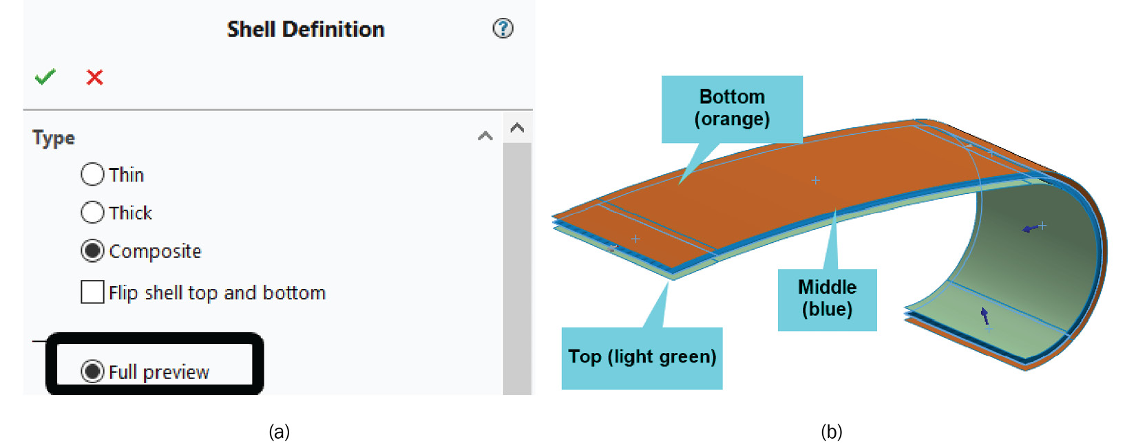
   Figure 8.17 – (a) The Full preview option and (b) revealing the shell top, bottom, and middle

   What immediately stands out from Figure 8.17 is that the shell's top and bottom faces are reversed. The light green color denotes the top face. Also, you will also notice that the shell is formed from the surface body by a middle offset method (which is why the ply in blue stays in the middle). We shall correct the position of the top and bottom faces in the next step.

3. Ensure the Full preview option is selected, and then tick inside Flip shell top and bottom (labeled 2 in Figure 8.18a). This flips the faces, as reflected in the graphics window:
   

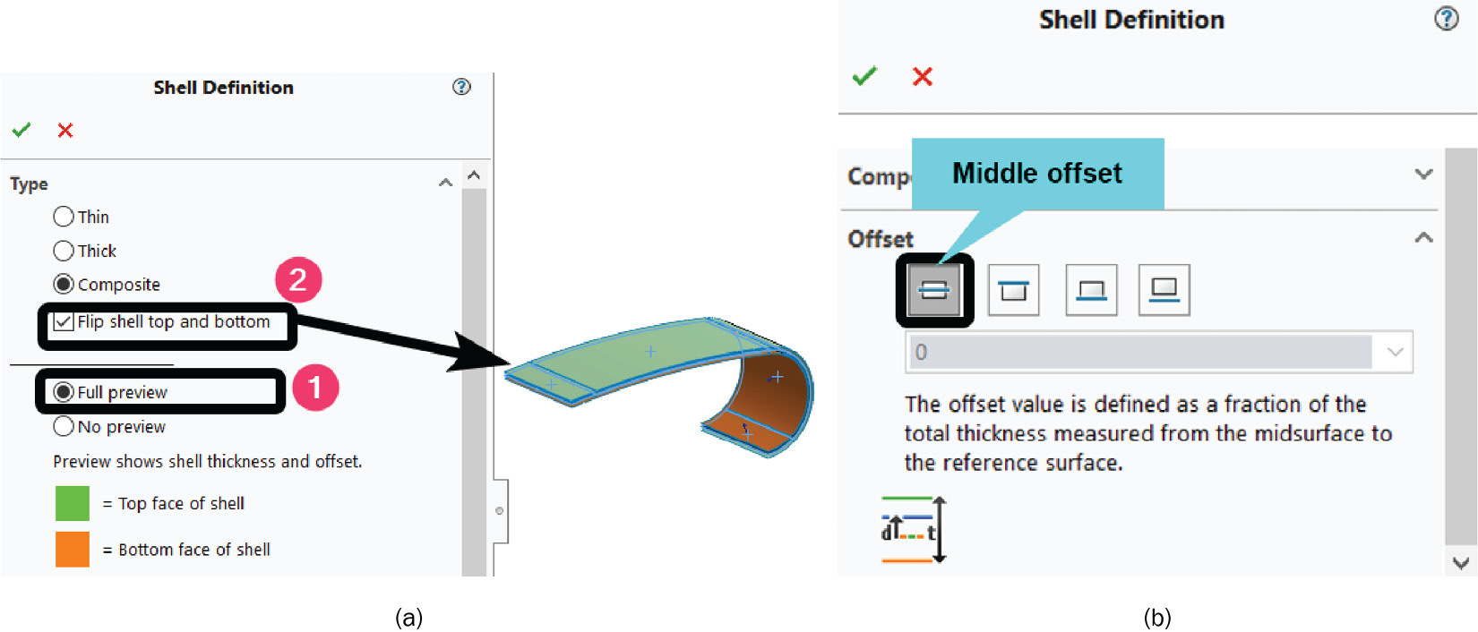
   Figure 8.18 – (a) Flipping the shell's top and bottom faces, and (b) revealing the Offset option

4. Next, to confirm the type of offset used to create the shell, scroll to the lower region of the Shell Definition property manager, and then expand the item named Offset. You will see that the middle offset option is depressed, as shown in Figure 8.18b. This step serves only as confirmation of this option. Don't make any changes, as the middle offset approach is often the preferred option to create shells. The other options may be used in cases where the middle offset option will lead to interference of a shell body with another body.

   Now that we have seen the offset and flipped the shell appropriately, let's examine another important feature in the next steps.

5. Scroll to the top of the Shell Definition manager, under Type, and select the No preview option. This will hide the top and bottom faces, and we can then see the fiber directions.
6. Within the Ply definition box, click on the first ply and note the update of the shell in the graphics window. You will see the fiber orientation and a coordinate system, as shown in Figure 8.19:
   

   Figure 8.19 – Revealing the fiber direction for ply one

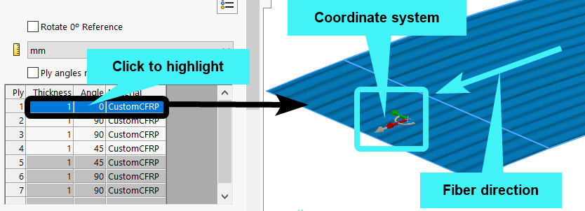
7. Next, click on the second and the fourth plies, one at a time. Each time, you will observe the shell is updated in the graphics window to show the fiber orientation, as shown in Figure 8.20a and Figure 8.20b for ply 2 and ply 4 respectively:
   

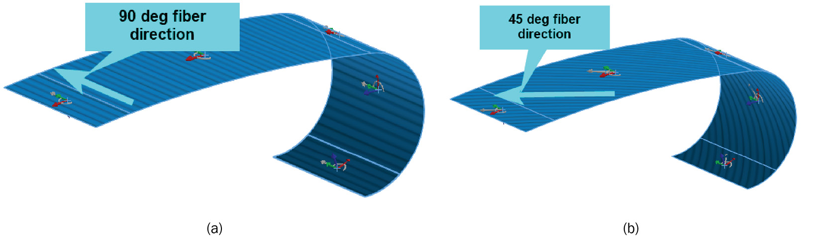
   Figure 8.20 – Revealing the fiber directions for plies two and four

8. Click OK to wrap up the examination.

At this point, we are done with the definitions of the composite shell properties. Specifically, we have created eight plies, each 1 mm thick and all made of CFRP. Note that the eight plies yield a total of 8 mm thickness for the overall composite laminate representing the elastic spring, which is the same as the dimension in Figure 8.4c. We have also examined some of the features and options that come with the definition of laminated composite shells. With this, we have provided a sufficient background to move ahead. Therefore, we will now shift our attention to the more familiar steps of applying the fixture and external load.

Applying the fixture and external load

The fixture for this case study involves the application of a fixed boundary condition on zone two of the surface. This zone is located at the bottom of the surface, as shown in Figure 8.5.

The steps to apply the fixture are outlined as follows:

1. In the Simulation study tree, right-click on Fixtures and pick Fixed Geometry from the context menu that appears.
2. When the Fixture property manager appears, navigate to the graphics window and click on zone two, as shown in Figure 8.21.
3. Click OK to complete the fixture specification:
   

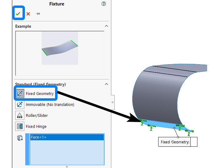
Figure 8.21 – Defining the fixed boundary condition in zone two

Now that we've completed the application of the fixture, let's move on to the application of the external load. This involves the application of a 100 N weight on the area designated as zone one in Figure 8.5.

The steps to achieve the application of the load are as follows:

1. Right-click on External Loads, select Force, and then follow the options indicated in Figure 8.22:
   

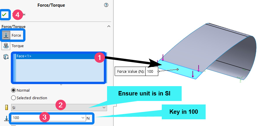
   Figure 8.22 – Options for the application of the force on zone one

2. Click OK to complete the application of the load.

At this point, we have established how to create and apply composite shell properties to a basic surface body. In effect, this involves the creation of a custom material with linear elastic orthotropic properties from scratch. We have also demonstrated how to assign the ply angles and thicknesses for the layers of a laminated composite. Moreover, we've completed the application of the fixture and the external load.

It is now time to get into the meshing phase of the simulation workflow.

Part C – meshing and modifying the system's options

By now, you have seen various ways to carry out the meshing of a structure. So, while this section briefly features the steps for the meshing, it also covers a small subsection that outlines the procedure to modify SOLIDWORKS Simulation's global options so that results can be displayed in the most preferable format later:

Meshing

The meshing strategy we shall adopt is to create the mesh directly without using mesh control. This is because the structure we have for this case study can be considered a simple structure that will be meshed with a single family of shell elements. For this reason, let's walk through the meshing as follows:

1. Right-click on Mesh and select Create Mesh.
2. From the Mesh property manager that appears, under Mesh Density, drag the Mesh Factor to the right, as shown in Figure 8.23:
   

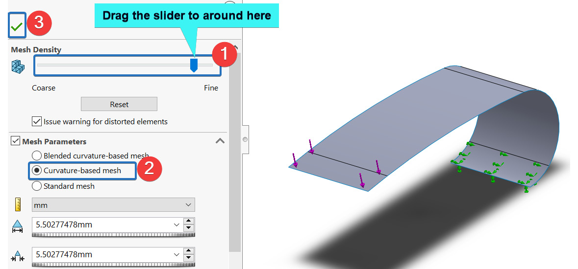
   Figure 8.23 – The mesh setting for the structure

3. Under Mesh Parameters, change the choice to Curvature-based mesh.
4. Click OK to complete the meshing actions.

The outcome of the preceding steps is the meshed structure portrayed in Figure 8.24a. After completing steps 1–4, you should check the mesh detail by right-clicking on Mesh and then selecting Details (the result of the mesh detail is shown in Figure 8.24b):

Figure 8.24 – (a) The meshed structure and (b) mesh details

This completes the meshing phase, which leaves us with the next set of actions geared toward modifying the simulation's global options.

Modifying the system options and running the analysis

Ordinarily, we would have dived straight into running the analysis, but the post-processing of results when dealing with an analysis that employs a composite material can get overwhelming. For this purpose, we shall streamline the way the results are displayed by modifying SOLIDWORKS Simulation's systems settings. The steps required for this are highlighted next:

1. From the main menu, click on Simulation, and then navigate to the lower part of the pull-down menu to click on Options, as shown in Figure 8.25:
   

   Figure 8.25 – Activating the simulation's options

2. From the Options property manager that pops up, navigate to the Default Options tab.
3. Click on Color Chart (labeled 2 in Figure 8.26).
4. Move the to the right side of the window, under Number format; change this to Floating (labeled 3 in Figure 8.26).
5. Click OK:

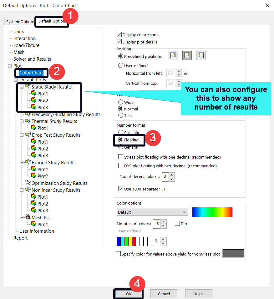
Figure 8.26 – SOLIDWORKS Simulation's system options

Many more options can be modified under the System Options and Default Options tabs. However, for the sake of brevity, we shall stick to this minor but important change. It is recommended that you look carefully at the various options; they will likely come in handy in your future explorations. In contrast to what we have done in the past chapters by accepting the default option, the change enacted in the preceding steps will save us the need to have to change the number format every time we retrieve a result.

With this, let's now transition to the running and retrieval of the results.

Part D – the running and post-processing of results

Overall, there are five subsections here to walk you through the running of the analysis and post-processing of the results.

Running the analysis and examining the default resultant displacement

Follow these steps to launch the solver:

1. Right-click on the study name and then select Run. After the running is complete, under the Results folder within the Simulation study tree, you will see the usual three default results (Stress 1, Displacement1, and Strain1).
2. Double-click on Displacement1 (-Res disp-) to display its plot in the graphics window, as shown in Figure 8.27:

Figure 8.27 – The plot of the resultant displacement

The plot in Figure 8.27 indicates that the maximum value of the resultant displacement is 5.119 mm. You may be puzzled by why we are getting the resulting displacement here rather than the vertical displacement along the Y axis. For this study, we are using a collection of shell elements to investigate the response of a composite-based component. Now, due to the variation in the fiber orientations of each ply in the laminated composite, the nodes of the discretized body are bound to experience complex movements along the X, Y, and Z directions. Consequently, the resultant displacement is a better indicator of the cumulative deformation of the composite structure than the vertical displacement along the Y axis (even though the load is normally applied solely to the surface in the Y direction). This is why it has been selected here. Meanwhile, take note that whatever values we obtain in this subsection belong to the composite laminate with the [0/90/90/45]s configuration shown in Figure 8.4c. We will later see in the Comparing displacements and stresses subsection how this compares with the second configuration in Figure 8.4d.

With the maximum resultant displacement value noted, we next aim to address the following questions:

• What is the maximum normal stress across the plies?
• What is the distribution of the factor of safety?

Obtaining the stress results

The following steps should be followed to obtain the maximum normal stress across the plies:

1. Right-click on the Results folder and then select Define Stress plot.
2. The Stress plot property manager should appear, as shown in Figure 8.28a:
   

   Figure 8.28 – (a) Examining the Stress plot property manager for composite analysis and (b) specifying options for the normal stress along the Z direction (major material direction)

   As you can see from Figure 8.28a, this Stress plot manager differs in appearance from what we have seen in the past chapters. The first difference is some newly available stress options that are specific to composite analysis, specifically the interlaminar shear stresses. Another notable difference is the option to configure the stress assessment for a specific ply, as shown under Composite Options in Figure 8.28a.

3. For the focus of this study, within the Stress plot property manager, under Display, follow the options highlighted in Figure 8.28b to retrieve the Maximum across all plies normal stress along the principal material direction. Note that you can iteratively examine the stress for each ply. However, for brevity's sake, we will not pursue this option. But it is recommended that you explore this further.
4. Click OK.

With the foregoing steps, the graphics window is updated with the plot of the normal stress along the Z direction, as shown in Figure 8.29:

Figure 8.29 – A plot of the normal stress along the Z axis (maximum across all plies)

From this plot, we can infer that the elastic spring experiences a maximum tensile normal stress across all plies of 32.711 MPa and a maximum compressive normal stress across all plies of -33.137 MPa. These values are relatively small compared to the strengths of the composite, which means the spring can sustain even more weight than the specified value of 100 N.

So far, we have retrieved the maximum resultant displacement and the maximum normal stress across all plies. Notably, the values we've obtained for these two important engineering design variables are not too excessive to raise concerns about the safety of the structure. Nonetheless, for a broader perspective on the performance of the design, we shall next examine the factor of safety.

Obtaining the factor of safety

Keep in mind that we discussed the Factor of Safety (FOS) in Chapter 2, Analyses of Bars and Trusses. There, we looked at the concept in the context of isotropic material. In contrast, for this study, we are dealing with an orthotropic fiber-reinforced composite material, which belongs to a family of materials with complex failure mechanisms. Nonetheless, irrespective of the material type used in calculating the FOS, two things should be clear:

• The FOS must be based on a certain failure criterion. As you will soon see, SOLIDWORKS Simulation provides three types of failure criteria for composite materials. These are the Tsai-Hill criterion, the Tsai-Wu failure criterion, and the maximum stress criterion. In what follows, we shall use the Tsai-Wu criterion. For more detailed coverage of the mathematical formulation behind these criteria, the excellent book by Hyer and White [4] is recommended.
• The greater the FOS is (than 1), the better the safety rating is of the component (all things being equal).

Now, to obtain the FOS, follow these steps:

1. Right-click on the Results folder and then select Define Factor of Safety Plot.
2. The Factor of Safety property manager appears, as shown in Figure 8.30a.
3. Under Composite Options, select Tsai-Wu Criterion, as indicated in Figure 8.30a:
   

   Figure 8.30 – (a) The first page of the Factor of Safety property manager and (b) The second page of the Factor of Safety property manager

4. Click on the Next arrow (labeled 2 in Figure 8.30a) to move to the second page of the property manager, which should appear as shown in Figure 8.30b.
5. Check the Worst-case across all plies box (labeled 1 in Figure 8.30b).
6. Click OK to exit the Factor of Safety property manager.

   The plot of the factor of safety will be displayed in the graphics window.

7. With the plot displayed, employ the Probe tool, as shown in Figure 8.31, and then navigate to the graphics window to pick four locations to assess the variation of the FOS:
   

Figure 8.31 – Using the Probe tool with the FOS

The final result of the FOS plot with four locations that have been picked is shown in Figure 8.32:

Figure 8.32 – The factor of safety based on the Tsai-Wu failure criterion

The summary table in the lower-left corner of Figure 8.32 indicates that the structure sustains a minimum FOS of roughly 14. This is a strong indication that the design is technically safe.

At this point, we have been able to address the questions that we set out to answer at the beginning of the problem about the values of the maximum resultant displacement, the maximum normal stress along the principal direction, and the minimum factor of safety. However, these values have only been obtained for the [0/90/90/45]s ply orientation of Figure 8.4c. For the sake of completeness, we will now briefly reckon with the second ply orientation (Figure 8.4d) in the next subsection.

Examining the response of the laminate with the ply set of [0/-45/45/90]s

The major thing we need to cover in this subsection is to determine the values of the resultant displacement and the maximum normal stress obtained for a laminate with the [0/-45/45/90]s orientation. This will allow us to determine whether there is any significant difference between the ply orientations.

Now, to analyze the new laminate orientation, we will duplicate the study we have completed in the previous sections so that we don't have to start the study from scratch.

To duplicate the study, follow the steps given next:

1. Navigate to the base of the graphics window, right-click on the study tab, and then select Copy Study, as shown in Figure 8.33a.
2. Within the Copy Study property manager that pops up, provide a name for the new study, for example, Prosthetics_ElasticSpring-Laminate2, as indicated in Figure 8.33b.
3. Click OK:

Figure 8.33 – (a) Duplicating the completed study and (b) naming the new study

After completing the preceding steps, a new study tab will be launched beside the old study tab. Ensure you remain in this new study environment. With the study copied, the next action is to edit the shell to reflect the new laminate configuration. The following steps show you how to edit the shell for the new study:

1. Within the Simulation study tree, right-click on the surface body and then select Edit Definition to open up the Shell Definition property manager (for a guide, you can refer to Figure 8.7).
2. Under Type, select the No preview option (if need be, see Figure 8.17a).
3. Navigate to the Ply definition box to update the ply angles, as shown in Figure 8.34. Note that only the angles of the top four plies need to be changed. It is recommended that you observe the fiber orientation on the shell as you modify the angles:
   

   Figure 8.34 – Updating the ply angles for the new laminate

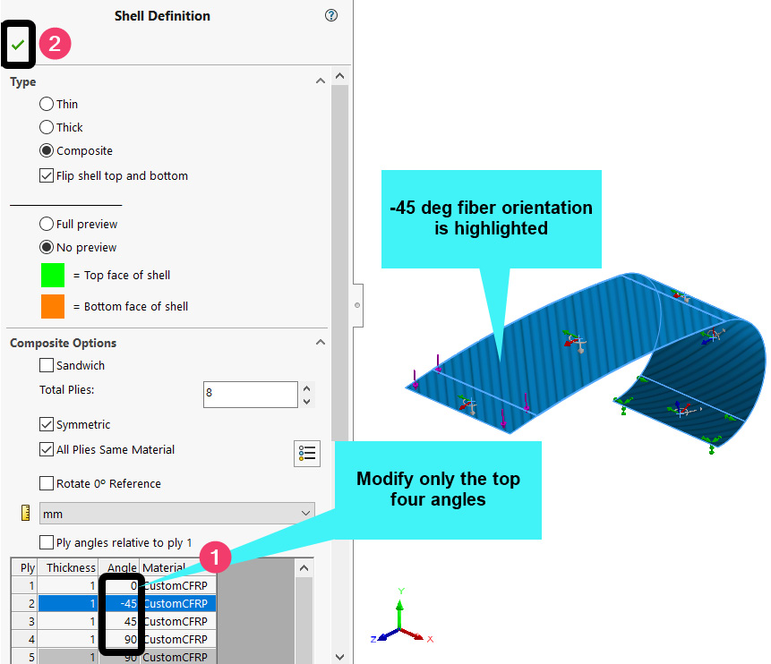
4. Click OK to wrap up the update of the ply angles.
5. Next, run the analysis by following Figure 8.35:

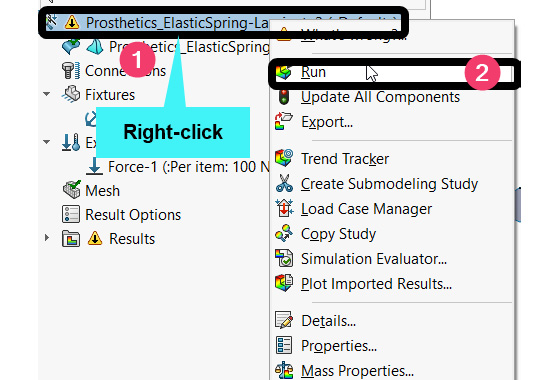
Figure 8.35 – Running the analysis with the new laminate set

After the running process is completed, we will have a new set of results. The key task for us now is to compare the results.

Comparing displacements and stresses

To compare the results of the analyses conducted with the previous laminate ([0/90/90/45]s) and the new laminate ([0/-45/45/90]s), follow these steps:

1. Right-click on the Results folder in the current analysis.
2. Select Compare Results (Figure 8.36a).
3. Within the Compare Results property window that appears, under Options, tick inside All studies in this configuration (labeled 1 in Figure 8.36b).
4. To compare the values of the resultant displacements from the two studies, make the selection as depicted in the box labeled 2 in Figure 8.36b.
5. Click OK to complete the selections for the comparison:

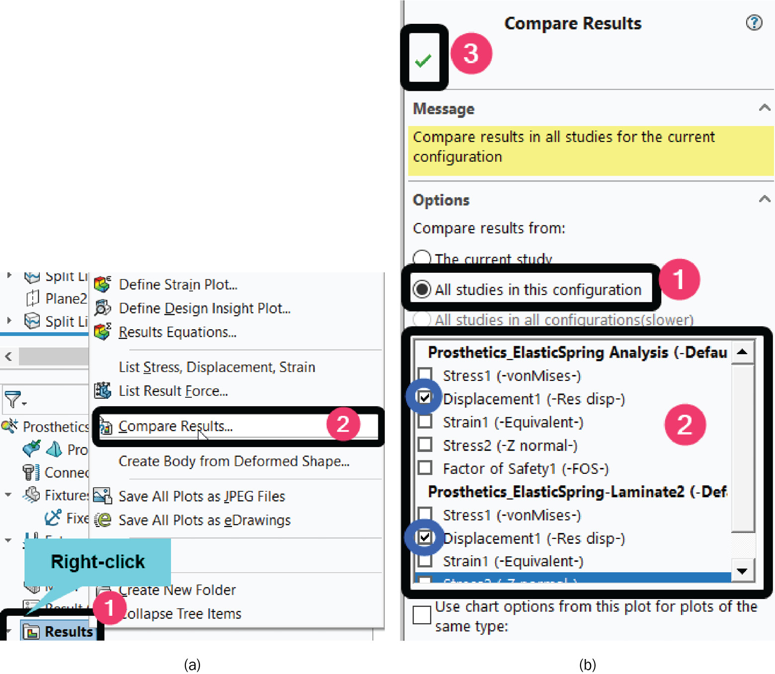
Figure 8.36 – Initiating the process of comparing the resultant displacements

Upon completing the preceding actions, the graphics window will be updated to show the plots of the resultant displacements for the two studies. This is shown in Figure 8.37:

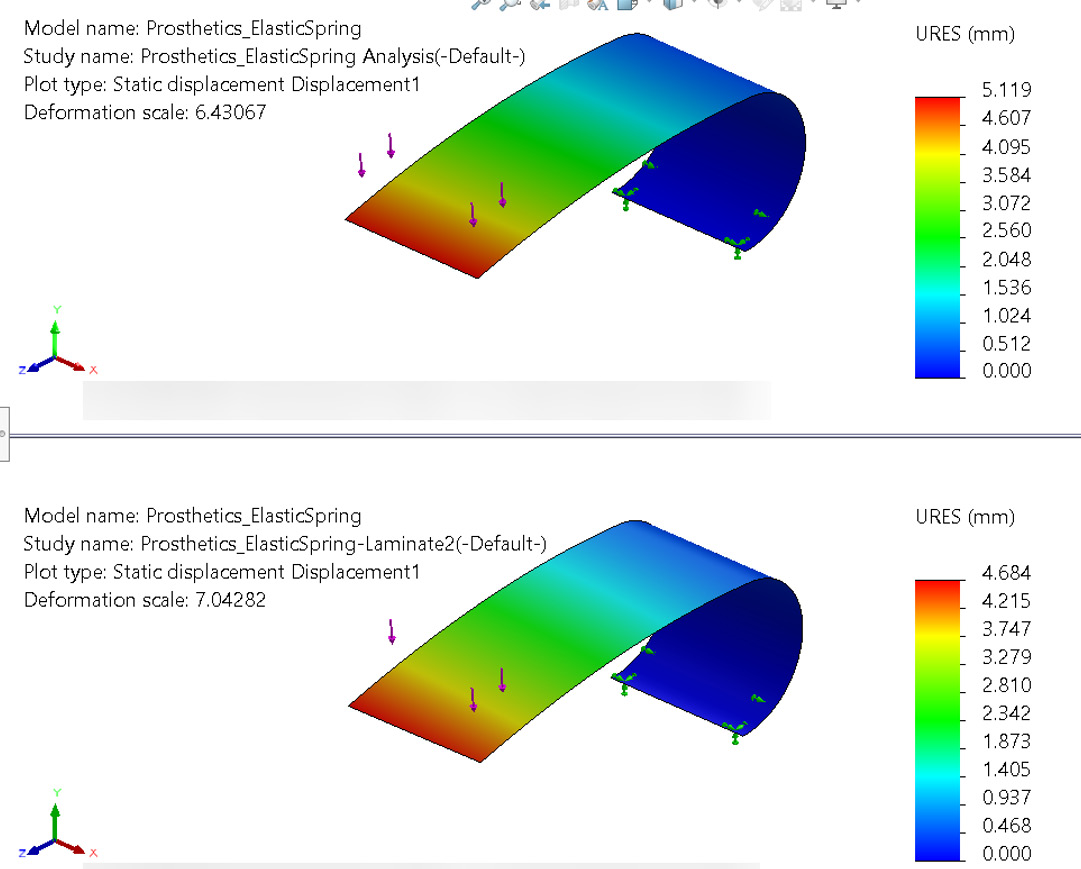
Figure 8.37 – The plots of the resultant displacements for the two studies

As you can see from Figure 8.37, the maximum resultant displacement for the laminate in the first study is 5.119 mm, while the maximum resultant displacement for the laminate in the second study is 4.684 mm. This difference amounts to a 9% lower deformation exhibited by the laminate with the ply set of [0/-45/45/90]s compared to that of the other laminate.

But can we say the same about the stress in the structure? Luckily, we can obtain a similar plot comparing the normal stress for the two studies. For this, you need to repeat steps 1–5. But instead of picking Displacement1(-Res disp-) for both studies (as was depicted in Figure 8.36b), pick Stress2 (-Z normal-) in step 4. With the steps executed, the outcome is shown in Figure 8.38 for the comparison of the normal stresses.

From the stress plots, it turns out that there is a relief of the compressive normal stress in absolute term with the [0/-45/45/90]s laminate, which experiences stress of 31.23 MPa compared to the 33.137 MPa that was experienced by the [0/90/90/45]s laminate. Meanwhile, the reality for the tensile stress is a bit different. The [0/-45/45/90]s laminate endures about 2% more tensile stress than what was induced in the [0/90/90/45]s laminate. All in all, given the lower deformation and the lower compressive stress, we can make the case that the [0/-45/45/90]s laminate offers a somewhat better static performance than the [0/90/90/45]s laminate.

As a final remark on this, in practical product design scenarios, ease of manufacturing will also feed into the decision to trade off one configuration of a laminate for another or one material for another. Occasionally, it may also be necessary to investigate the fatigue behavior of both laminates in addition to the basic stress/deformation analyses conducted here. We shall look at fatigue analysis in Chapter 9, Simulation of Components under Thermo-Mechanical and Cyclic Loads:

Figure 8.38 – The plots of normal stress along Z for the two studies

This concludes our exploration of the case study. Through this case study, we have touched on important concepts to give you the background to build on concerning the analyses of components with composite materials. Over the many sections, you have seen the creation of a custom orthotropic composite material, the application of a composite material to a laminate, the definition of ply properties, and the visualization of fiber orientations. Also, you have learned the difference between the types of stress and failure criteria available for analyses with composite materials. Finally, we have leveraged the Compare Results tool in SOLIDWORKS Simulation to compare the performance of laminates with different sets of ply orientations. In the next section, we shall take a brief look at some other points to be mindful of in the simulation of advanced composite structure.

Analysis of advanced composite structures

The world of analysis with composite materials is vast. So far, in the completed case study, we have dealt with a component constructed of an 8-ply laminate, with all plies having the same material (which is CFRP). For advanced composite structures, things can get pretty complex. For this reason, among other things, you need to know the following:

• In SOLIDWORKS Simulation, you can only have a maximum of 52 plies.
• If you have a total number of plies, say n, take note that SOLIDWORKS's ply-counting procedure starts from the bottom surface (ply 1) to the top surface (ply n).
• You can have each ply derived from different materials, not just one material.
• You can have complex geometric bodies with intersections. Nevertheless, no matter how complex a structure may be, to analyze it with a composite material, it must be created as a collection of surface bodies.

With this achieved, you can leverage the skills and workflow demonstrated in the previous sections to explore the analysis of advanced composite structures.

Summary

We started this chapter with an overview of composite materials as they relate to the analysis of composite structures. We finish having conveyed fundamental concepts for the static analysis of composite structures using the SOLIDWORKS simulation capabilities. Using a composite elastic spring in the case study, we have demonstrated, among other things, the following:

• How to convert a basic surface body into a composite shell
• How to create a custom orthotropic composite material, assign its properties to a composite laminate, and visualize the fiber orientations of composite plies
• How to obtain the stress cross plies and employ the right failure criteria to assess the factor of safety for composite structures
• The benefit of editing the global simulation settings to enhance the presentation of results

By bringing the knowledge of this chapter and the previous chapters together, you have acquired the foundational skill set to be able to handle the various kind of analyses of composite structures. In the next chapter, you will learn about the analysis of components with thermo-mechanical and cyclic loads.

Exercise

1. Re-conduct the case study to compare the performance of the [0/-45/45/90]s and [45/-45/45/90]s laminates. By using the same load and boundary condition, determine the percentage difference in the resultant displacements engendered by both laminates. What is the difference in interlaminar stress between the two?
2. Re-conduct the case study to investigate the performance of the elastic spring with a laminate of the [0/90/90/0]s form. How does it compare with [0/-45/45/0]s in terms of deformation?

Further reading

• [1] Materials Selection in Mechanical Design, M. F. Ashby, Elsevier Science, 2016
• [2] A parametric study of flutter behavior of a composite wind turbine blade with bend-twist coupling, Composite Structures, Vol. 207, P. Shakya, M. R. Sunny, and D. K. Maiti, pp. 764–775, 2019
• [3] Introduction to composite materials, Stability and Vibrations of Thin Walled Composite Structures, H. Abramovich, Elsevier, pp. 1–47, 2017
• [4] Stress Analysis of Fiber-reinforced Composite Materials, M. W. Hyer and S. R. White, DEStech Publications, Incorporated, 2009
• [5] A multi-purpose prosthetic fitness foot, Ottobock, https://www.ottobockus.com/fitness/solution-overview/challenger-foot/, (accessed 2021)