
Chapter 6: Analysis of Components with Solid Elements
This chapter builds on the idea of advanced elements within the SOLIDWORKS simulation library that we commenced looking at in the preceding chapter. Primarily, the current chapter hones in on solid elements, versatile elements for the simulation of arbitrary three-dimensional bodies. In the course of exploring these elements with two concrete examples, the chapter features the use of mesh control, the setting up of global/local interactions between components, the significance of curvature-based meshes, and an assessment of contact stress, among other things. Overall, the following topics will be covered:
- Overview of components that deserve to be analyzed with solid elements
- Analysis of helical springs
- Analysis of spur gears
Technical requirements
You will need to have access to the SOLIDWORKS software with a SOLIDWORKS Simulation license.
The sample files used in this chapter can be found here:
Overview of components that deserve to be analyzed with solid elements
As an analyst, you will be confronted with a wide range of simulation tasks, and the onus will be on you to decide on the most appropriate element as part of the finite element simulation workflow. Choosing the right element has an enormous impact on the accuracy of your simulations.
In the context of static analysis, the solid element remains one of the most flexible elements suitable for the analysis of various kinds of components. In the previous chapters, we mentioned some limitations of the truss/beam/shell elements when they were introduced. Although these elements allow us to use fewer elements in our simulations, they are all mathematical and mechanistic approximations of three-dimensional (3D) bodies. Therefore, in practice, a set of solid elements can be used whenever the structure you wish to analyze violates the limitations of structural elements such as beam/shell elements. For instance, anytime the dimensions of components are comparable to each other, then adopting solid elements for discretization becomes necessary (although not sufficient).
The set of engineering components that can be sufficiently analyzed with solid elements is vast. This ranges from simple to geometrically complex engineering structures and machinery. Figure 6.1 shows some examples of components that can be analyzed with solid elements:
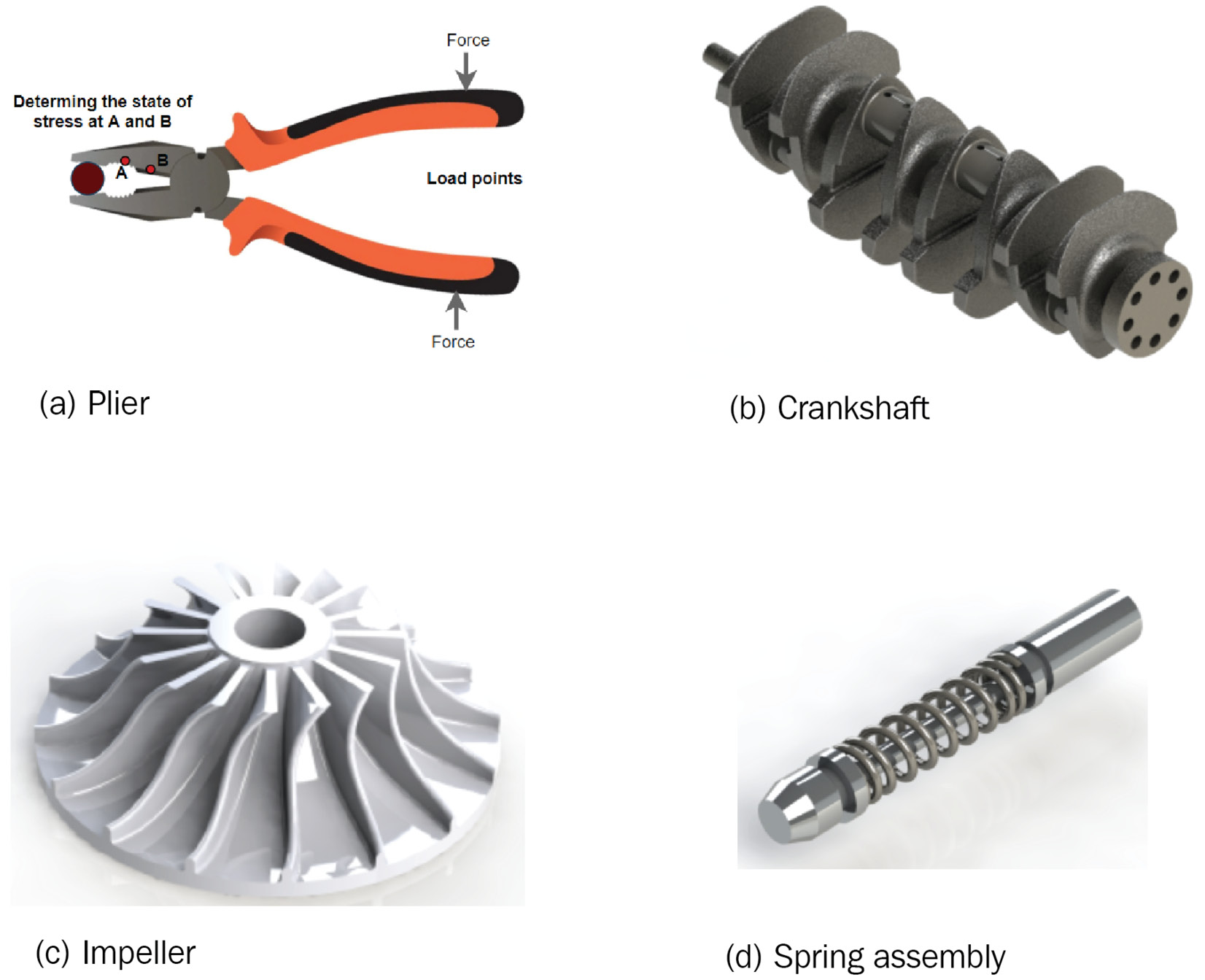
Figure 6.1 – Some examples of structures that may require solid elements for analyses
Among the group of seemingly simple components that needs to be analyzed with solid elements is the following non-exhaustive list:
- Non-prismatic beams with variable geometric details
- Short and thick beams/shafts/plates/panels with structurally significant stress raisers in the form of perforations, cut-outs, fillets/chamfers, grooves, keyways, and so on
- Thick-walled tanks, pipes, and cylinders with complicated connections and support effects
- Axisymmetric bodies with non-symmetric loads/supports/material properties
- Machine elements in the form of springs, gears, and so on
Examples of structures within the category of geometrically complex engineering components and machinery are far too numerous to list. A few examples include machinist vise, T crane hook, crankshaft, pliers, impeller, heavy-duty lifting brackets, and so on.
Now that we have gotten the basic background out of the way, it is time to bring into the picture some details and strategies necessary for the analysis of general 3D bodies.
Structural details
The primary technical details needed for the analysis of 3D bodies are again similar to those we listed in the previous chapters. These include the following:
- The dimensions of the component (for an assembly, the dimensions of all members)
- Material properties (the assumption of the isotropic material property is again adopted in this chapter)
- External loads applied to the component/assembly
- Supports provided to the component/assembly
Next, we will touch upon a few tricks to simplify or modify components for analysis with solid elements.
Model simplification strategies
It is impossible to have a list of all-encompassing strategies to be adopted for the simplification of components to be analyzed with solid elements. Nevertheless, three basic strategies that have wide applications are listed here:
- Model simplification via suppression: This strategy involves suppressing features that perform purely aesthetic or less structural functions before launching the simulation study environment. Such features comprise fillets, chamfers, decals/embossed text, cosmetic threads, and so on. For instance, the fillets and chamfers in Figure 6.2a have been suppressed in Figure 6.2b:
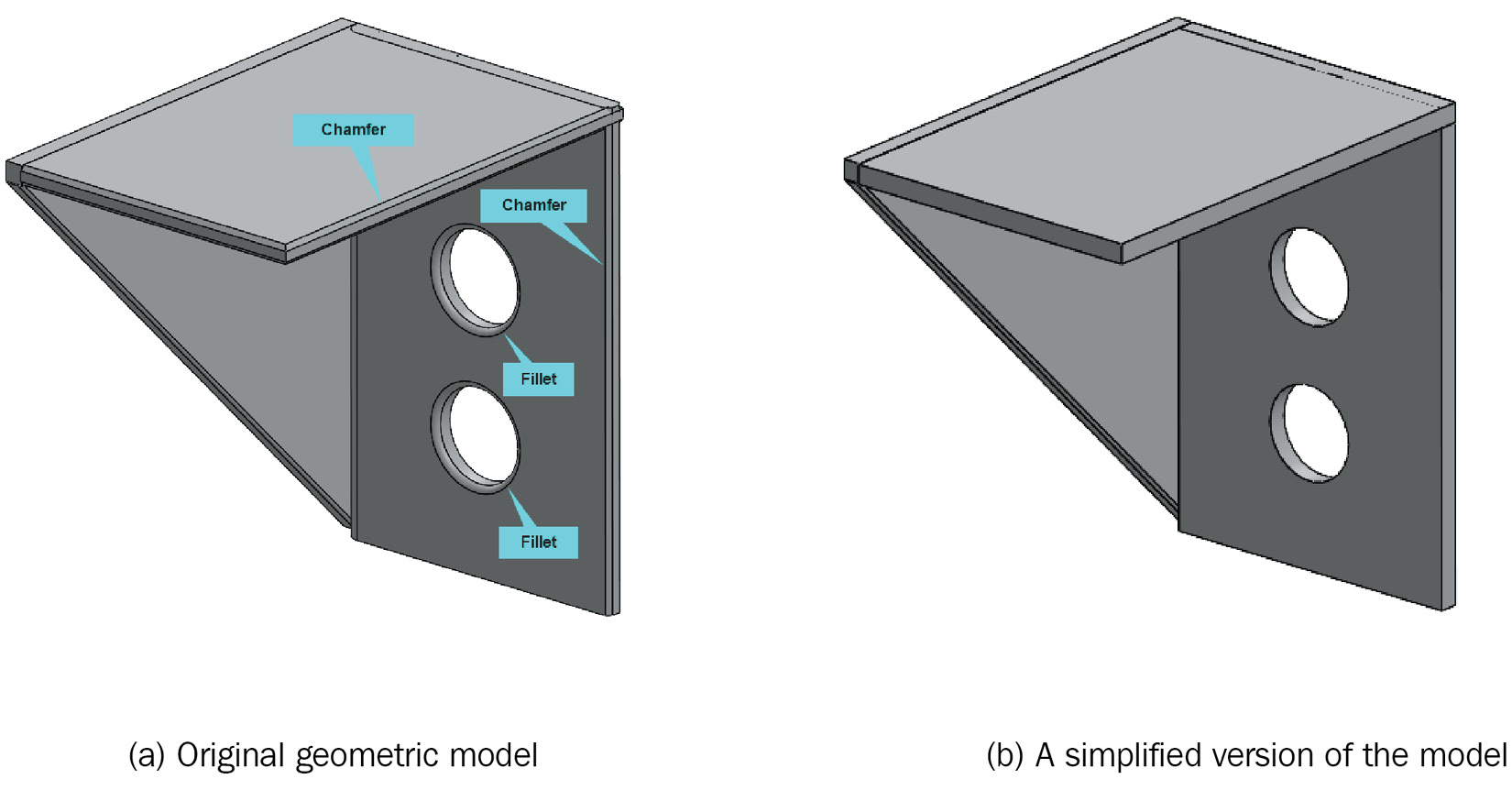
Figure 6.2 – An illustration of the suppression of fillets and chamfers
Note that feature suppression can be done manually or with the automated option within the simulation environment.
- Defeaturing: For very large components with a horde of small features and small aesthetic parts, the manual suppressing approach becomes time-consuming and almost impractical. Besides, for large assemblies, you may have to deal with small aesthetic features that are hidden within several connecting parts. In such scenarios, it is better to fall back on the automated approach that relies on the SOLIDWORKS defeature command. This can be accessed from the main menu (Tools Defeature).
The two strategies outlined so far demand that we remove certain features to simplify the model, but we can also add some subtle features that will simplify the downstream finite element simulation tasks. One such kind of addition is discussed next.
- Addition of split line/reference point/reference axis: These three features (split line, reference point, and reference axis) are very useful for the creation of a partial face, an arbitrary point, or a desired axial line for the application of loads/supports on solid bodies. As with the previous approaches, these features are created before launching the simulation study. Figure 6.3 illustrates two scenarios where a split line and a reference point are added to the model to allow the application of distributed and point loads:
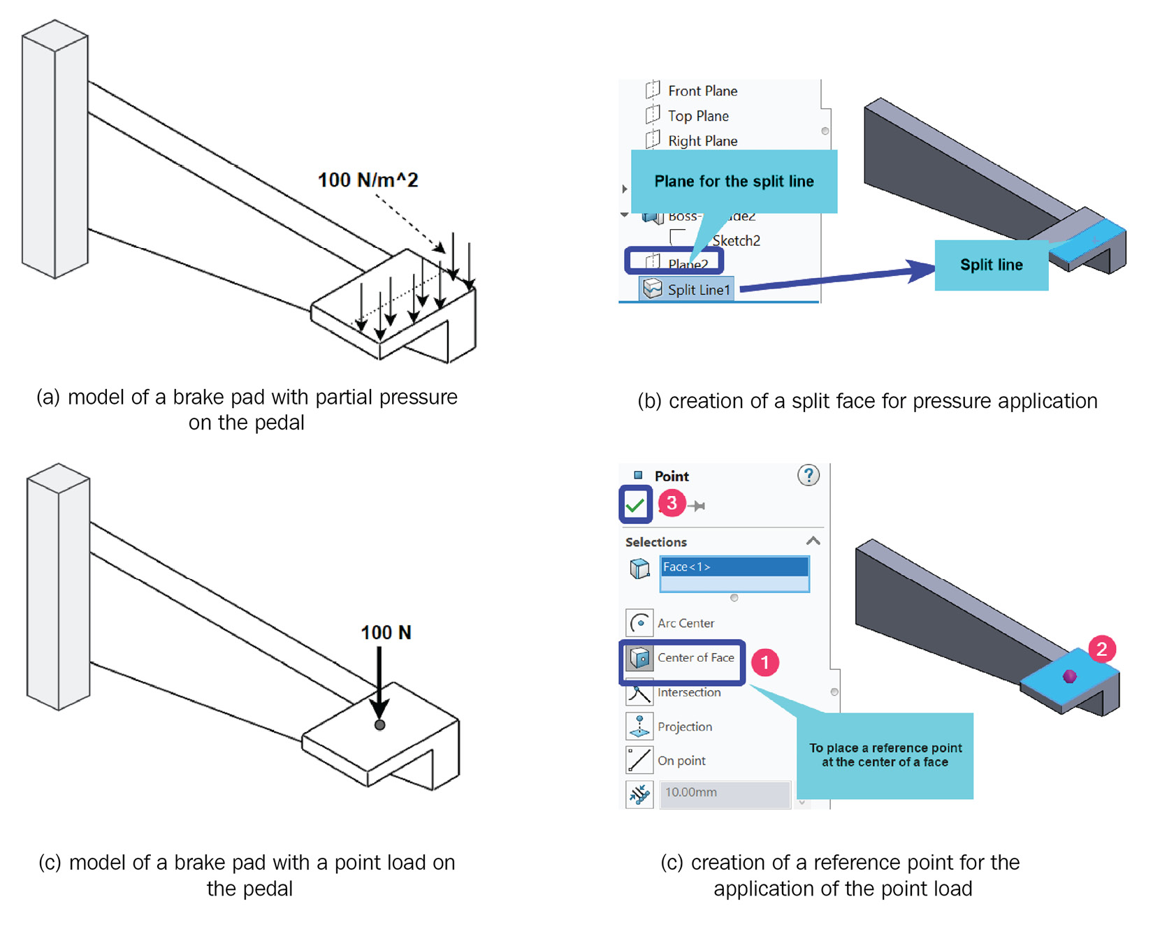
Figure 6.3 – Addition of a split line/reference point for load applications
In a way, the addition of a split line, reference points, and reference axes on solid bodies mirror our use of critical positions in Chapter 3, Analyses of Beams and Frames.
Before we get to the case study, let's touch a little bit on a few attributes that solid elements possess.
Characteristics of solid elements
The first attribute is that solid elements are truly 3D sub-domains with well-defined volume data. Another is that they sit atop the family tree of continuum elements (discussed in Chapter 1, Getting Started with Finite Element Simulation). Furthermore, two popular categories of solid elements are widely used in finite element simulations (Figure 6.4): (i) the hexahedron-based solid elements – a 3D extension of the 2D quadrilateral elements that are also sometimes called brick elements; and (ii) the tetrahedron-based solid elements – a 3D extension of the 2D triangular elements. In terms of usage, in most cases, a collection of tetrahedral elements is suitable for the analysis of irregular solid bodies. However, in the absence of irregular features (such as corners, grooves, keyways, and so on), a collection of hexahedral elements will provide better accuracy and will often require less simulation runtime compared to tetrahedral elements.
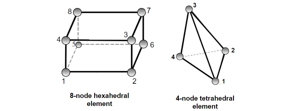
Figure 6.4 – An illustration of the shapes and nodes of hexahedral and tetrahedral elements
Note that only tetrahedral solid elements are available in SOLIDWORKS.
As with the shell element discussed in Chapter 5, Analyses of Axisymmetric Bodies, two formulations of the tetrahedral solid element exist within the SOLIDWORKS simulation library:
- The first-order (4-node) tetrahedral solid element (also referred to as a linear solid element)
- The second-order (10-node) tetrahedral solid element (also referred to as a parabolic solid element)
Now, as a consequence of being 3D and belonging to the family of continuum elements, each nodal point of the aforementioned solid elements has only three translational displacement degrees of freedom along the X, Y, and Z axes. They do not have rotational degrees of freedom.
Note
For further explorations of the mathematical formulations of solid elements, you may consult the books by Koutromanos [1] (see the Further reading section), Reddy [2], and Hutton [3], among others.
Drawing on the ideas we have presented so far, we will now dig into the exploration of two case studies that will allow us to employ solid elements in our simulation. The first is on helical spring, while the second relates to spur gears. The two case studies will showcase some new concepts, for instance:
- How to create and prepare a variable pitch spring for analysis
- Recognizing the pitfalls of the standard mesh
- How to simplify a multi-body component/assembly by excluding some components from the analysis
- How to set up a "no penetration" contact and obtain contact stress
We begin with the first case study in the next section.
Analysis of helical springs
Our first case study is a simulation exercise that involves a helical compression spring. Springs are known to store energy when deflected and return the same energy upon release from the deformed state. Their use can be found in systems as complex as vibration isolation systems, shock absorbers, watches, and bomb detonation mechanisms, to simple devices such as toy cars and pens. Detailed accounts of the design of springs can be found in some of the references in the Further reading section, for example, [4]. In what follows, we will examine the simulation of a helical compression spring as part of a sub-assembly.
Problem statement – case study 1
Figure 6.5 shows different views of a spring-based weighing module. The performance of the module is intrinsically tied to the deformation of the compression helical spring (isolated in Figure 6.5c). As a result, understanding the performance of the spring is a necessary engineering design task. The spring is to be made from an ASTM316 stainless steel wire with a diameter of 10 mm. Other data about the spring are listed here:
- Total number of active coils = 10
- Number of inactive coils = 4
- Free length of the spring = 500 mm
- The outside diameter of the spring = 100 mm
The spring is ground at the ends. The objective is to compute the deflection and the maximum shear stress experienced by the spring when a load of 25 kg is placed on the load carrier (see Figure 6.5b). The load carrier weighs 500 g, resulting in a pre-load of 5 N. Further, we wish to know how well the deflection and the shear stress retrieved from our simulation compare with the theoretical expressions for springs' deflection and shear stress developed by Wahl [5].
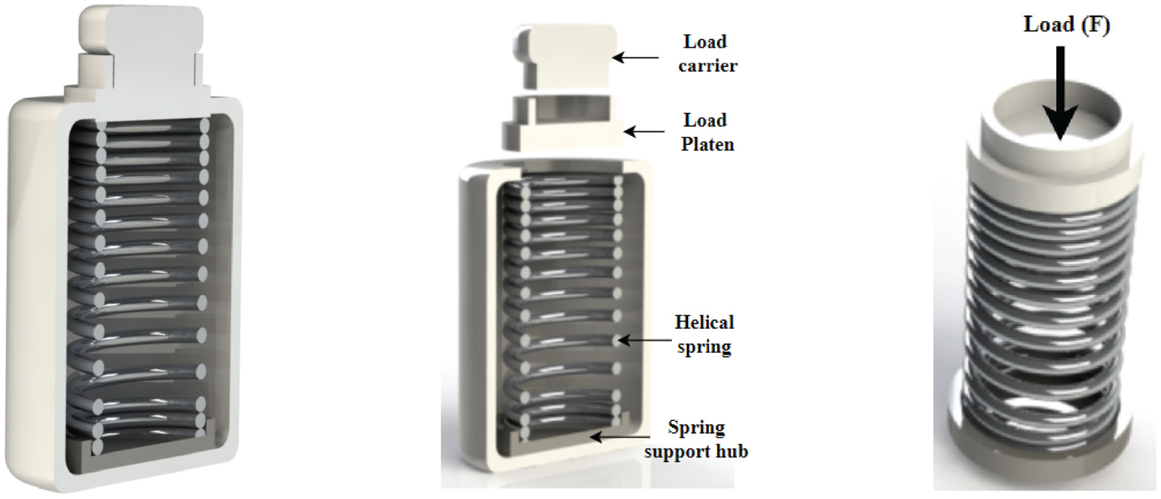
Figure 6.5 – Spring-based weighing system: (a) a sectioned view of the simplified assembly; (b) an exploded view showing the major components; (c) the spring sub-assembly
In what follows, we will walk through a systematic procedure to create and analyze the spring sub-assembly in Figure 6.5c. As in earlier chapters, we will address the solution to the above problem in three major sections designated as Part A: Creating the model of the spring sub-assembly, Part B: Creating the simulation study, and Part C: Meshing and post-processing of results.
Let's begin with the modeling phase.
Part A: Creating the model of the spring
There are three components we will use for the simulation: (a) the helical spring; (b) the spring support hub; and (c) the load platen. Figure 6.6 shows the major geometric dimensions of these components:
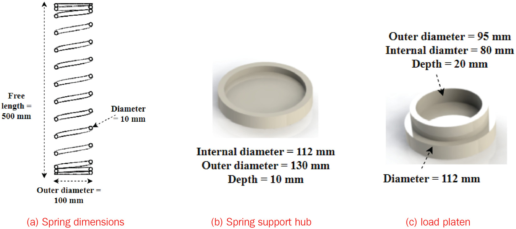
Figure 6.6 – Dimensions of components
Due to space limitations, the explanation that follows focuses squarely on the creation of the variable pitch spring (since the other components are easy to model).
To commence, start up SOLIDWORKS (File New Part). You are encouraged to save the file as Spring and ensure the unit is set to the MMGS unit system.
Creating the helix profile of the variable pitch spring
The backbone of the spring is the helix guide curve. The helix can be generated by specifying the following geometric details [6, 7]:
- A reference circle matching the diameter of the helix
- The height of the helix, which should correspond with the free end of the spring
- The pitch, which describes a distance between identical points along the axial direction of the helix
- The revolution, which describes the number of complete turns of the helix
So, let's begin by sketching the reference circle of diameter 100 mm on Top Plane by taking the following steps:
- Navigate to the Sketch tab.
- Click on the Sketch tool.
- Choose Top Plane.
- Use the Circle sketching command to create the circle as depicted in Figure 6.7.
Ensure the center of the circle is positioned at the origin of the coordinate system.
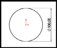
Figure 6.7 – Reference circle for the helix (100 mm diameter)
- Launch the Helix/Spiral property manager from the main menu via Insert Curve Helix/Spiral.
- Within the Helix/Spiral property manager that appears, create the helix guide curve with the details shown in Figure 6.8:

Figure 6.8 – Completing the helix profile
Notice that we have used the Variable pitch option (under Parameters) in Figure 6.8. You will also notice the preview of the helix. Notice that the first two coils and the last two coils will act as inactive coils.
With the completion of the helix profile, we will now add the cross-section of the spring wire.
Creating a new plane and the cross-section of the spring wire
The cross-section of the wire is 10 mm. However, to create this cross-section, we need a new plane. For this purpose, follow the steps listed next to create the new plane for the cross-section:
- Navigate to the Features tab.
- Click on Reference Geometry, and then select Plane (Figure 6.9a).
From the Plane property manager that appears (after completing step 2), complete the creation of the plane by following the next steps.
- Click inside the First Reference box (labeled 1 in Figure 6.9b), then navigate to the graphics window and pick the helix curve.
- Click inside the Second Reference box (labeled 2), then navigate to the graphics window and pick the starting point of the helix curve.
- Click OK.

Figure 6.9 – Creating a reference plane for the cross-section
Steps 1–5 will create the plane. With the plane created, follow the steps listed next to create the 10 mm diameter cross-section.
- With the new plane still active, use the Circle command to complete the sketching of the circle as shown in Figure 6.10:

Figure 6.10 – Creating a 10 mm circle on the new plane
We now need to position the center point of the circle at the starting point of the helix. We will do this by adding a pierce relation between the sketched circle and the helix curve.
- For the Pierce relation command to appear as shown in Figure 6.11a, hold down the Ctrl key, and then select the center of the circle. While still holding down the Ctrl key, click near the starting point of the helix (don't aim for the starting point). The pierce property manager should appear.
- Click on the Pierce relations command (labeled 3), and then click OK.

Figure 6.11 – (a) Applying the pierce relation; (b) illustration of the pierced circle/curve
With the cross-section snapped in place, we are now set to extrude the profile along the curve.
For this purpose, follow the steps listed next to use the Swept Boss/Base command to complete the extrusion:
- Navigate to the Features tab and select the Sweep Boss/Base command.
- Under the Profile and Path section, select the options indicated in Figure 6.12a.
- Click OK.
By completing the preceding steps, you will get a model of the spring as shown in Figure 6.12b:
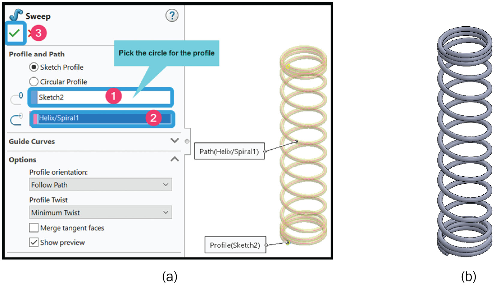
Figure 6.12 – Options for creating the sweep profile
We have now completed the basic model of the helical spring. But we are still left with three more details (somewhat minor but important) about our model of the spring sub-assembly. These are as follows:
- The end treatment: This is what will give us the ground/flat ends. This eases the positioning of the spring as it interacts with other members of the assembly.
- A reference axis: This allows us to read the stress value across a section of the curve.
- The models of the spring hub/load platen: This will allow us to apply load and boundary conditions indirectly on the spring.
Note about End Treatment
For a variety of applications, it is common to subject compression helical springs to some form of end treatment. You can read more about this from any book on machine element design, for instance, the book by Mott [4] or from websites on spring design such as https://www.acxesspring.com or https://www.leespring.com.
We will now briefly engage with the creation of the end treatment.
For brevity's sake, the next set of steps offers a brief guide for the completion of the model. To create the end treatment and the reference axis, we will need to generate a set of intersection curves, which is the next task.
Adding construction intersection curves
Follow the steps given next to create the intersection curves:
- Move to the Feature Manager tree, then click to activate Right Plane.
- Right-click on the right plane to choose Normal To (Figure 6.13a).
- Navigate to the Sketch tab and then select Intersection Curves under the Convert Entities command.
- When the Intersection Curves property manager comes up, follow the illustration in Figure 6.13b to complete the generation of the intersected curves:
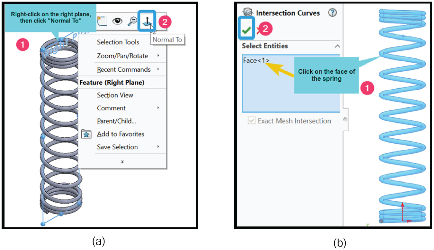
Figure 6.13 – Creating the intersection curves
After you are done with the Intersection Curves command, a projection of the cross-sections that intersect the right plane will be formed as shown in Figure 6.14a.
- Select all the generated curves/circles (use the box selection approach) and convert them to construction sketches by ticking the For construction option (labeled 2 in Figure 6.14b).
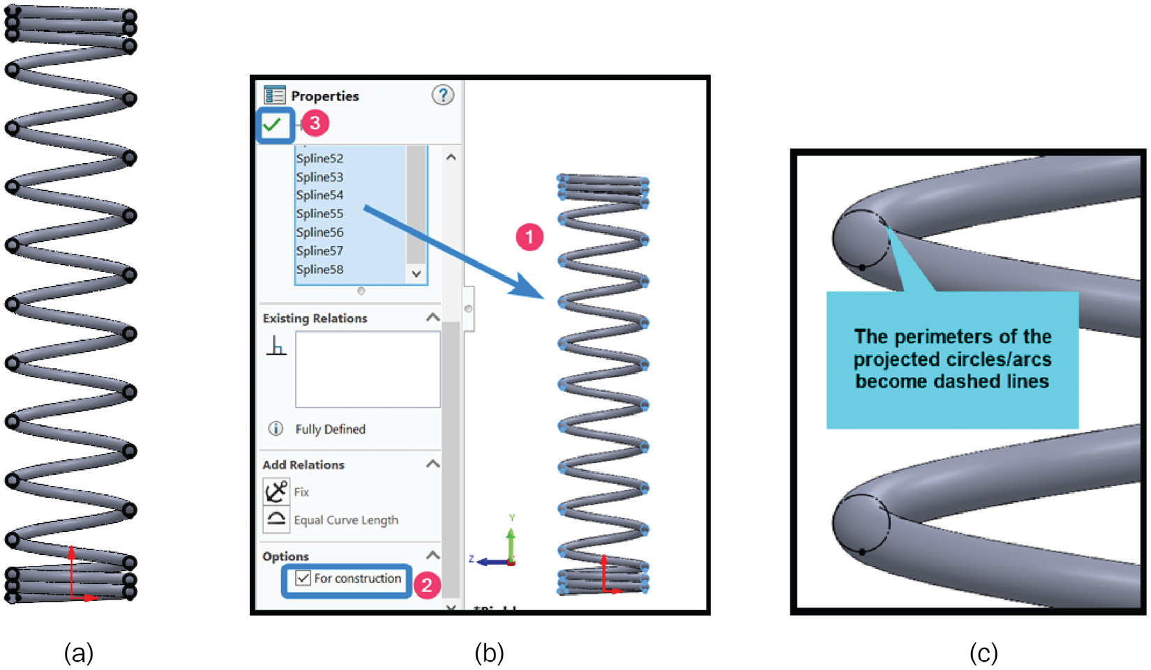
Figure 6.14 – Conversion of the intersection curves into construction sketches
After step 5 is complete, you may zoom in on the converted circles/curves. You should notice their perimeters have turned into dashed lines as shown in Figure 6.14c.
We are now done with the creation of the construction intersection curves. How do we use the curves we've created? That is the focus of the next sub-section.
Adding the end treatments and reference axes
According to the problem statement, the spring is ground at the ends. We will use the Extruded Cut command to replicate the grounding of the spring's ends. The steps for doing this are as follows:
- Using the tangent points on the converted arcs at the bottom and top of the spring, create the rectangles with the Corner Rectangle command as shown in Figure 6.15a.
- Activate the Extruded Cut command from the Features tab. This will launch the Cut-Extrude property manager (Figure 6.15b).
- Complete the options within the Cut-Extrude property manager (Figure 6.15b).
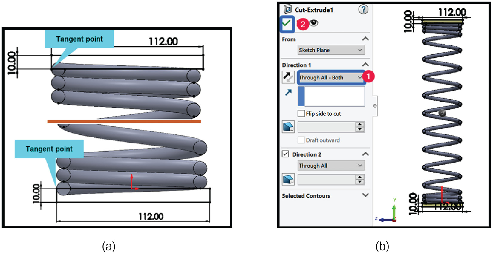
Figure 6.15 – Creating the end treatment
Next, we will add two reference axes. Each one will pass through any of the converted curves we created earlier. The steps to achieve the addition of the reference axes are given next:
- Create a new sketch on the Right Plane (the same as steps 1–5 in the sub-section Adding construction intersection curves).
- Use the Centerline command to create two line sketches across any two of the circles (one is shown in Figure 6.16a). Ensure you exit the sketch mode after completing the line sketches.
- Create two reference axes to coincide with the two lines created in step 2 by selecting Insert from the main menu, and then Reference Geometry Axis.
Figure 6.16b shows the two reference axes created:

Figure 6.16 – Adding two reference axes
We have now completed the final status of the spring. One last thing we need to cater to is the creation of the spring hub base and the load platen. You may use the dimensions provided in Figure 6.6(b and c) to create these items as shown in Figure 6.17a. Notice that in Figure 6.17b, a reference point is placed at the center of the face to allow us to apply a point load later on. In any case, a complete model of the sub-assembly is available for download if you've any difficulty in completing the model shown in Figure 6.17. Primarily, the components of the sub-assembly are modeled in place (which means they were just placed on each other in one part file) with no interacting mates between them.

Figure 6.17 – Model of the spring sub-assembly
This brings us to the end of the modeling of the spring sub-assembly. We will now shift our focus to tackle the simulation tasks.
Part B: Creating the simulation study
The simulation workflow again comprises all the necessary pre-processing routines (the activation of the simulation study, assigning of material, application of fixtures, and the specification of loads).
We begin with the activation of the simulation environment.
Activating the Simulation tab and creating a new study
To activate the simulation commands, we follow the steps highlighted next:
- Click on SOLIDWORKS Add-Ins.
- Click on SOLIDWORKS Simulation to activate the Simulation tab.
- With the Simulation tab active, create a new study by clicking on New Study.
- Input a study name within the Name box, for example, Spring analysis.
- Keep the Static analysis option.
- Click OK.
As soon as we complete steps 1–6, you will see the simulation environment with the compartmentalized sections as shown in Figure 6.18:
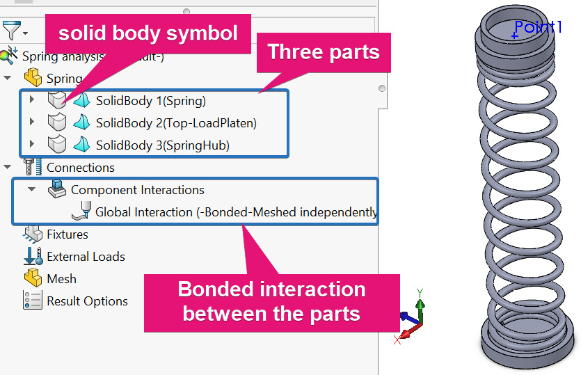
Figure 6.18 – Simulation property manager
As seen in Figure 6.18, we have three parts. One of the remarkable features of SOLIDWORKS Simulation is that, once you launch a simulation study, most parts are automatically treated as solids (unless converted otherwise). What this means is that we do not have to make any conversion of the three imported parts. Recall that in Chapters 2, Analyses of Bars and Trusses to Chapter 4, Analyses of Torsionally Loaded Components, we manually converted the bodies to trusses/beams. We also did a conversion to a shell in Chapter 5, Analyses of Axisymmetric Bodies. Since we want to use solid elements for our discretization, we will therefore accept this default behavior.
It's time to shift our attention to the application of materials.
Assigning the materials
For the purpose of simplification, the spring, the spring hub, and the load platen are taken to be made of ASTM316 stainless steel (this may not be the case in a real design).
Follow the steps given next to assign the material to the three bodies at once:
- Right-click on the parts folder (named Spring) and choose Apply Material to All Bodies (Figure 6.19).
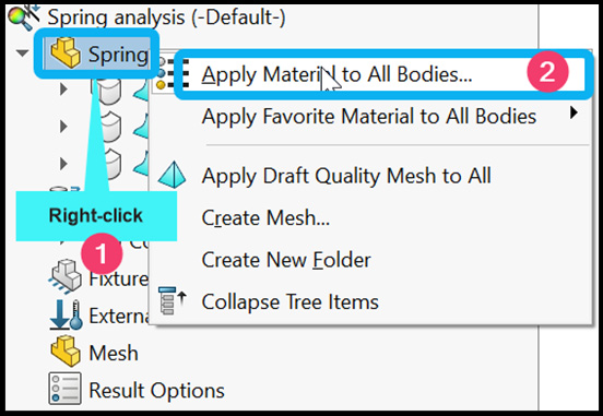
Figure 6.19 – Assigning material to the bodies
- From the materials database that appears, expand the Steel folder.
- Click on AISI Type 316L stainless steel.
- Click Apply and Close.
The material assignment task is now completed. In the next sub-section, we will briefly take a look at the contact/interaction setting (before we deal with the application of the load and the specification of the fixture).
Examining the interaction setting
Since we have three parts that are interacting with each other, contacts must be defined between them. Now, given that the parts are designed to have faces that are touching each other, SOLIDWORKS has explicitly defined a contact for us.
To verify, let's examine this contact option:
- Within the simulation study tree, expand the Connections folder, and then right-click on Global Interaction (Figure 6.20a).
- From the Component Interaction property manager that appears, keep the options as shown in Figure 6.20b.
As indicated in Figure 6.20b, a combination of Bonded interaction with the option to Ensure common nodes between touching boundaries has been chosen. The Bonded option selected here ensures the parts remain fully attached during the simulation (you don't want a situation where the spring runs away from the load platen).

Figure 6.20 – Examining the interaction details
For more details about the other options, see Chapter 4, Analyses of Torsionally Loaded Components, in the sub-section Scrutinizing the interaction settings. There is so much on interaction/contact settings that we will come back to them in the second case study. We will also re-visit them in Chapter 7, Analyses of Components with Mixed Elements. Nevertheless, this wraps up the examination of the interaction settings.
It is now time to apply the fixture.
Applying the fixture at the base of the spring hub
Our boundary condition for this problem is simple: just a fixed support at the base of the sub-assembly. The steps to apply the fixture are as follows:
- Right-click on Fixtures.
- Pick Fixed Geometry from the context menu that appears (Figure 6.21a).
- When the Fixture property manager appears, navigate to the graphics window and click on the bottom face of the sub-assembly as shown in Figure 6.21b.
- Click OK.

Figure 6.21 – Defining the fixed boundary condition
With the completion of the application of the fixed boundary condition, let's now move on to the application of the force at the top of the spring sub-assembly.
Applying the external load
To apply the force, follow the steps outlined next:
- Under the simulation study tree, right-click on External Loads and select Force.
Within the Force/Torque property manager that appears, execute the next actions.
- Click inside the Force reference box (labeled 1 in Figure 6.22a) and navigate to the graphics window to click on the reference point at the center of the load platen.
- Check the Selected direction option (labeled 3 in Figure 6.22a).
- Click inside the direction reference box (labeled 4 in Figure 6.22a), and then navigate to the graphics window to choose Right Plane.
- Under Force, input 255 in the box labeled 5 (Along Plane Dir 2) and ensure the unit system remains as SI.
- Click OK.
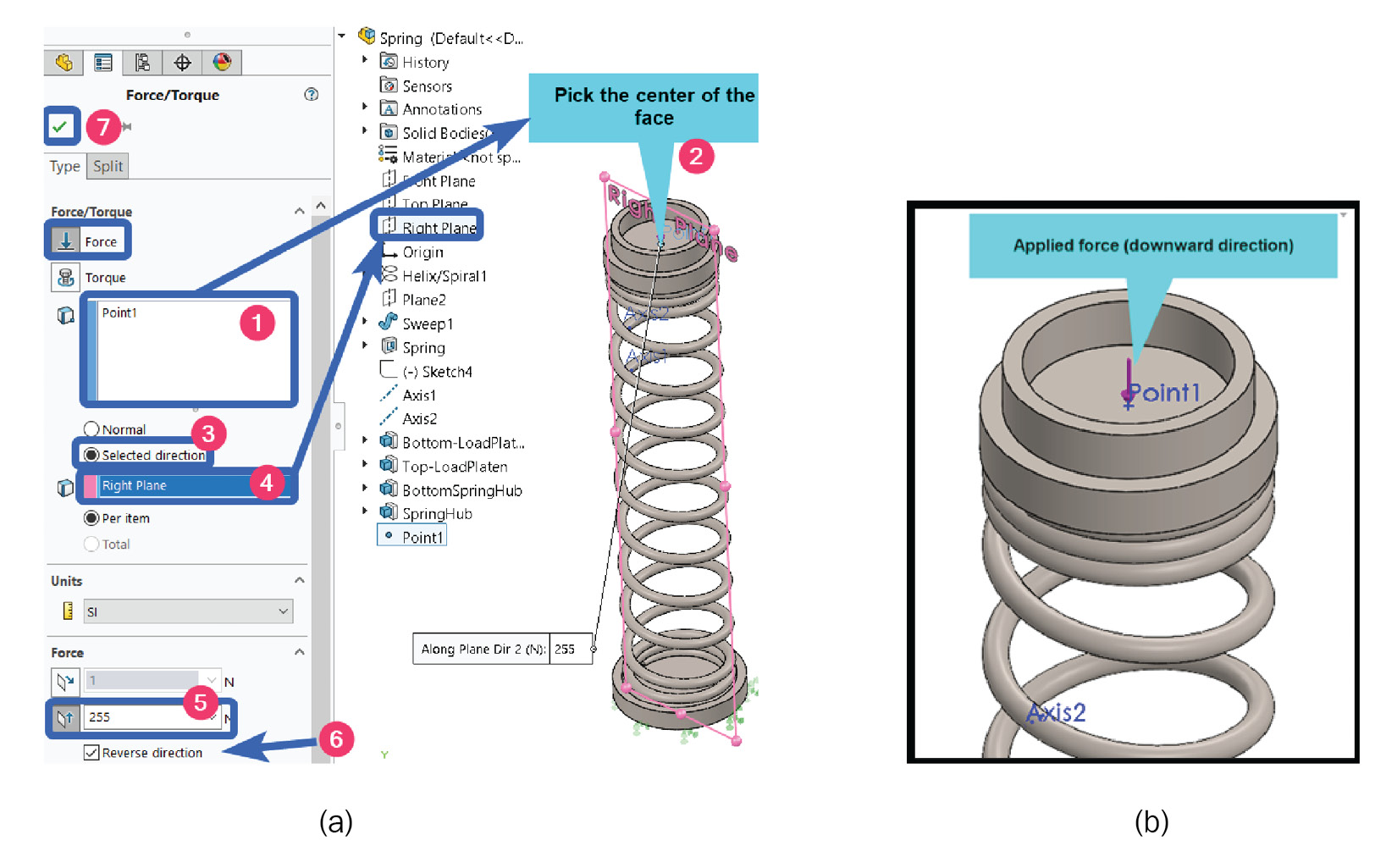
Figure 6.22 – Initiating the application of the point load
Figure 6.22b shows the arrow of the applied load. You will notice that we have applied a force of 255 N in step 5. This is derived from the conversion of the 25 kg mass to weight (250 N). This is then combined with the pre-load of 5 N coming from the weight of the load carrier.
At this point, we have covered the creation of a variable pitch helical compression spring. We have examined the state of the body as solid within the simulation environment. We have assigned a material, applied the necessary fixture, and applied the point load to the spring sub-assembly. We are therefore set for the meshing task and running of the analysis, which is what happens in the next section.
Part C: Meshing and post-processing of results
This sub-section is devoted to meshing. As stated in Chapter 5, Analyses of Axisymmetric Bodies, when dealing with advanced elements, the mesh quality has a profound effect on the accuracy of our results. Furthermore, as we are dealing with a spring in this analysis, it is worth exploring that a wrong choice of mesh type can also make or break a simulation workflow. So, in what follows, we will examine the difference between the meshes created by the Standard Mesher and the Curvature-based Mesher. In simple terms, the meshes created by the former are called standard meshes, while those of the latter are known as curvature-based meshes.
Examining standard and curvature-based meshes
Begin the meshing procedure by following the steps given next:
- Right-click on Mesh within the simulation study tree and then select Create Mesh.
The Mesh property manager appears, using which you need to make the following selections.
- Under Mesh Density, drag the Mesh Factor control bar (labeled 1 in Figure 6.23a) to the right (indicating a fine mesh).
- Under Mesh Parameters, go with the default choice of Standard mesh.
- Click OK.
By completing step 4, you are likely to get a message indicating a failed mesh as shown in Figure 6.23b, although the other two components are meshed easily (indicated by the green grids).
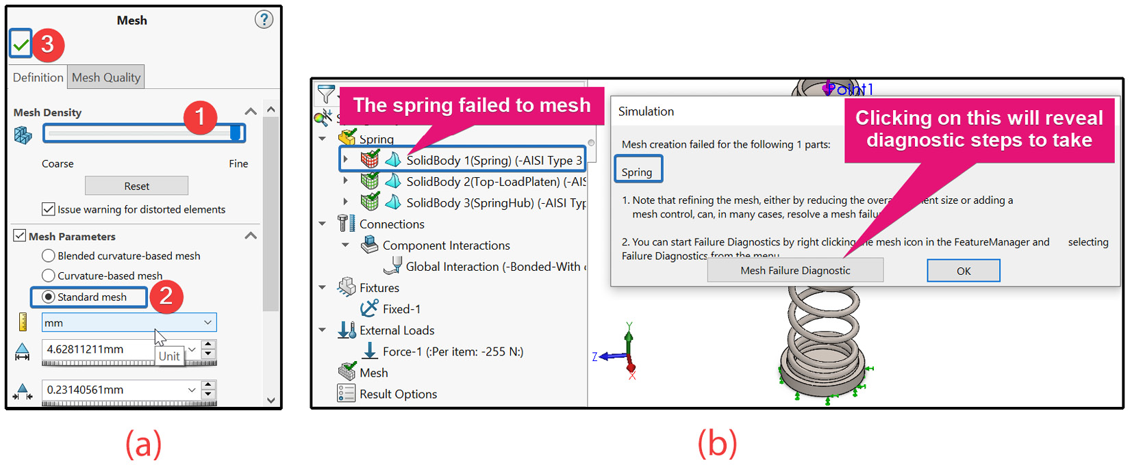
Figure 6.23 – (a) Options to create a fine standard mesh; (b) evidence of mesh failure
The message in Figure 6.23b suggests that the mesh failure is due to the spring. When you encounter this kind of failed meshing operation, clicking on the Mesh Failure Diagnostic button will take you to another window stipulating steps to take to correct the issue.
However, for this problem, we know that a major reason the mesh failed for the spring hinges on its extreme curvatures. The curved segments of the spring cannot be easily discretized using the standard mesh. We now have two options:
- The first option is to do mixed discretization. With this, the spring will be discretized using the curvature-based mesh approach and the other two components are discretized with the standard mesh.
- The second approach (and easy route) is to re-discretize all three components with the curvature-based mesh. Let's go with the second approach.
The steps to upgrade to a curvature-based mesh are briefly outlined here:
- Right-click on the Mesh folder within the simulation study tree and select Create Mesh.
- Complete the options as indicated in Figure 6.24a:
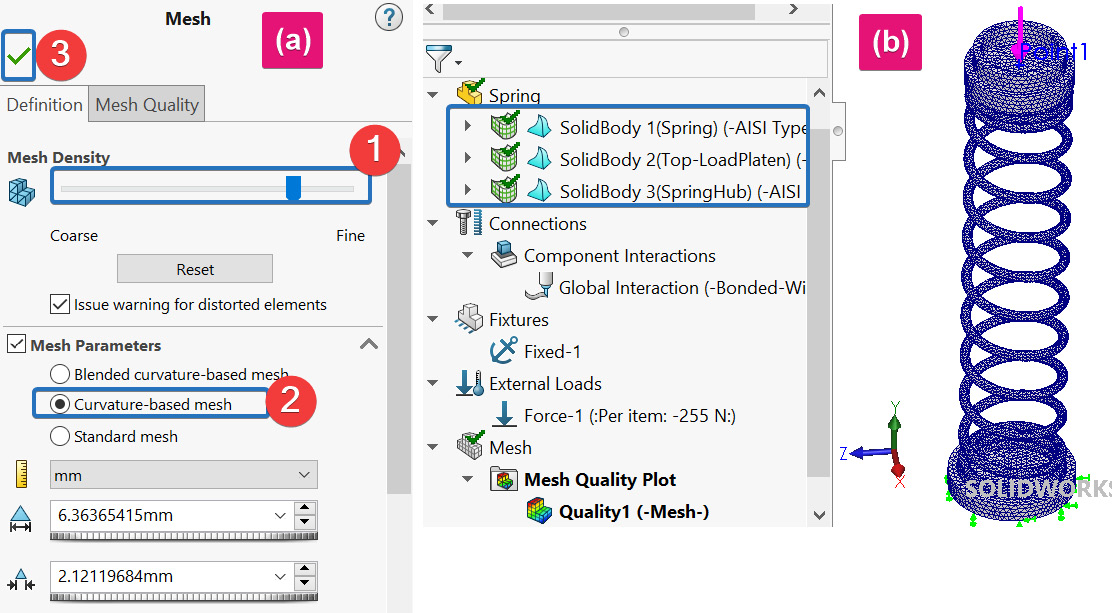
Figure 6.24 – (a) Options to obtain the curvature-based mesh; (b) the meshed solid bodies
As expected, completing the steps for the curvature-based mesh discretized all three bodies with no difficulty, as shown in Figure 6.24b. Why does the curvature-based mesher handle discretization easily? Well, the elements produced by this mesher are based on parabolic tetrahedral solid elements, which are more robust than the linear tetrahedral elements of the standard mesher.
Meanwhile, by virtue of the position of the mesh slider (labeled 1) in Figure 6.24a, you will notice that we are using a less than fine mesh. The mesh quality can be fine-tuned if our result is not satisfactory. But waiting to see the result before knowing whether the mesh is good for the analysis is not optimal. The trick is to use the mesh detail feature of SOLIDWORKS Simulation.
Therefore, let's take a look at the mesh detail, which we have not done in any of the previous chapters. To get the mesh detail, simply right-click on the Mesh folder and then select Details (Figure 6.25a). Doing so will reveal the features of the mesh shown in Figure 6.25b:

Figure 6.25 – Examining the mesh details
What can we garner from Figure 6.25b? We can get the following details:
- We have generated a set of solid elements (referred to as Solid Mesh in the figure).
- We have created the meshes using the curvature-based mesher.
- We have generated a total number of elements that equals 71,395 and created a number of nodes that equals 123,478.
- We managed to have the Maximum Aspect Ratio for the element as 7.9601.
A good rule of thumb to know whether you have a relatively good mesh is to ensure the maximum aspect ratio is not more than 20. Luckily, this condition is satisfied by our mesh. For complex models, it is not uncommon to run into a situation in which the aspect ratio of some elements will be more than 20. In such scenarios, you will need to use Mesh Control to refine the discretization in the region where this happens. We will use Mesh Control in case study 2 later in this chapter.
Having come this far, we are ready to run the analysis and retrieve the results that we want.
Run the analysis
Follow the steps given next to accomplish the running operation:
- Right-click on the study name and then select Run (Figure 6.26a).
- You may get a suggestion about allowing the use of the Large Displacement option. Select No (Figure 6.26b).

Figure 6.26 – (a) Initiating the running of the analysis; (b) suggestion to use the Large Displacement option
Note
Note that although we are neglecting the warning about excessive displacement here, the warning is telling us something about the design. Excessive deformation for a linear elastic material could lead to instability and should be checked in a normal design task. This warning will appear mostly when the maximum displacement/characteristic length of the structure being analyzed exceeds 10%.
Once the running process is complete, we will then be able to retrieve the desired results. Primarily, we are interested in the following:
- Determining the deflection experienced by the spring when the total load of 255 N is applied to it
- Finding the maximum shear stress developed in the spring
- Finding out how well the shear stress computed by the simulation compares with theoretical expressions
Let's commence with the retrieval of the deflection result.
Obtaining the deflection of the spring
We are interested in the displacement of the spring in the vertical direction (that is, along the Y-axis). To obtain this value, carry out the following steps:
- Right-click on the Results folder and then select Define Displacement Plot.
- We will now update some of the options within the Displacement Plot property manager that appears.
- Under the Definition tab, navigate to Display and keep the options as shown in Figure 6.27a.
- Now, move to the Chart Options tab, and then, under Position/Format, change the number format to floating, as depicted in Figure 6.27b.
- Click OK.
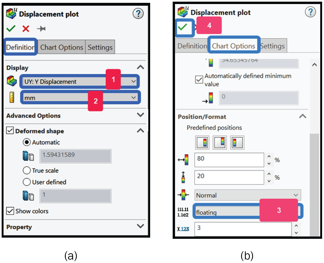
Figure 6.27 – Specifying options for the displacement plot
By completing steps 1–5, the graphics window will be updated with the plot of the vertical displacement, as shown in Figure 6.28:
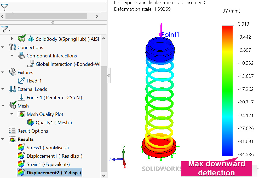
Figure 6.28 – Distribution of the displacement across the three bodies
Figure 6.28 indicates that the maximum downward deflection happens to be -34.5 mm, which is at the upper region of the assembly, while the lower region experiences negligible deflection (which makes sense because it is fixed). Meanwhile, note that the maximum value is for the whole sub-assembly. Clearly, we will want to know the deformation experienced by the spring. For this purpose, we will fall back on the use of the Probe tool, as outlined next.
Using a Probe with the displacement
Follow these steps to retrieve the average value of the displacement on the spring:
- Right-click on Displacement2 (-Y disp-).
- Select Probe from the resulting menu.
- Keep the options in the Probe Result property manager as depicted in Figure 6.29.
- Navigate to the graphic window and click on four points on the face of the spring in the upper region (see Figure 6.2).
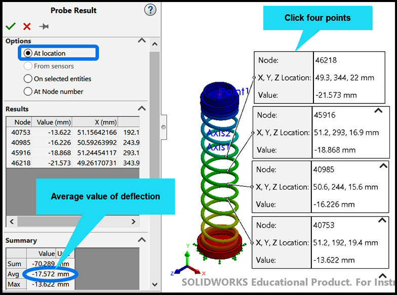
Figure 6.29 – Options for Probe Result and the average displacement value
You will notice a table summarizing the displacement values in the lower-left corner of the Probe Result window, as shown in Figure 6.29. The Summary table indicates that an average value of -17.572 mm is experienced by the spring.
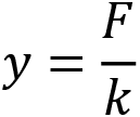
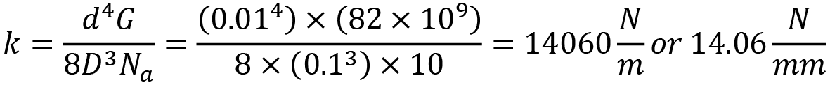
But what can we say about the accuracy of this number? As is often the case, we can borrow some knowledge from the theories of the design of machine elements. For instance, for a spring with a wire diameter (d = 10 mm), a mean diameter (D = 90 mm), number of active coils (Na = 10), shear modulus (G = 82 x 109 Pa), and an applied force (F), the deflection (y) can be predicted from equation 6-1 (see Further reading [4]):
 (6-1)
(6-1)
Where k is the spring rate defined by:
 (6-2)
(6-2)
With k found (in equation 6-2), and F = 255 N, then y = 255/14.06 = 18.13 mm. As you can see, this value only differs by less than 1% from what we got from our SOLIDWORKS simulation. This brings us to the end of the discussion on the deflection of the spring.
We will now obtain the shear stress.
Obtaining the shear stress across the cross-section
Take the actions listed next to obtain the shear stress:
- Right-click on the Results folder and then select Define Stress Plot.
Now let's modify the options within the Stress plot property manager (summarized in Figure 6.30) that appears.
- Under the Definition tab, navigate to Display and select TXY: Shear in Y Dir.
- Within the unit box (labeled 2 in Figure 6.30), change the unit to N/mm^2 (MPa).
- Under Advanced Options, check the box labeled 3 (Show plot only on selected entities).
- Under Advanced Options, click on the body symbol (labeled 4) and then navigate to the graphics window to click on the spring.
- Under Advanced Options, click inside the box labeled 6 and then navigate to the graphics window to select one of the reference axes (you may repeat the step for the other reference axis).
- Click OK.
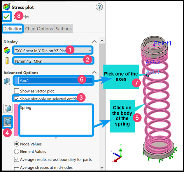
Figure 6.30 – Specifying options for the shear stress plot
By completing the preceding steps, you should obtain a plot similar to Figure 6.31:

Figure 6.31 – Variation of the shear stress
On the one hand, it can be seen from Figure 6.31 that the maximum shear stress happens to be roughly 75.708 MPa. On the other hand, the maximum positive shear stress happens in the interior of the spring.
We will now compare the shear stress from the simulation with the theoretical equation for shear stress in a spring, which was originally derived by Wahl [5]:
 (6-3)
(6-3)
where 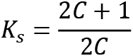 , and it referred to the shear correction factor. Besides C = D/d (the spring index), the other parameters are as defined in the earlier equations. Substituting the values for all the parameters into the equation 6-3 yields 71.42 MPa.
Again, the theoretical value of the shear stress and that obtained from the simulation are very close, confirming the accuracy of the simulation setup. Recall that we have used a less than fine mesh, so the gap is likely to close with further refinement of the mesh. You are encouraged to try this to confirm.
This concludes the simulation of the first case study. This specific case study has taken us on a journey that sees us modeling a helical spring, preparing it for downstream simulation tasks. Furthermore, we have obtained, examined, and validated the displacement and shear results obtained for the spring.
Before we wrap up the chapter, we will go through another case study in the next section.
Analysis of spur gears
The central objective of this section is to analyze the spur gears assembly. We will focus narrowly on the qualitative assessment of the stress arising from the interaction of the gears' teeth. Among other things, this case study will enable us to see the application of a local interaction contact and the use of mesh control.
Problem statement – case study 2
Figure 6.32a shows the assembly of a gear-shaft system for a power transmission train. The gears are made of plain carbon steel. The purpose of this case study is to examine the stress that develops due to the contact between the teeth of the gears when gear A rotates by 1.15 degrees, while gear B is retrained.
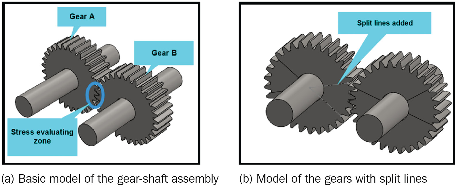
Figure 6.32 – A gear-shaft assembly
To address the simulation task concisely, two models of the assembly are provided for this problem. Download the Chapter 6 folder from the book's GitHub repository. Inside the folder, you will see the first assembly file (named Gear-Assembly), which is the basic model shown in Figure 6.32a. The second assembly file is named Gear-Assembly-Split, and is the one shown in Figure 6.32b, where split lines are added to facilitate mesh control and a stress plot. In what follows, the second assembly file will be used for the analysis.
Launching SOLIDWORKS and opening the gear assembly file
Here, we start by opening the assembly file in SOLIDWORKS (File Open Gear-Assembly-Split). Ensure the unit is set to the MMGS unit system.
Once the assembly is opened, it is good to check any interference between the parts.
Follow the steps given next to check the interference of the assembly:
- Navigate to the Evaluate tab, and click on Interference Detection (Figure 6.33a).
This launches the Interference Detection manager, inside which we take the steps that come next.
- Within the Selected Components box (labeled 1 in Figure 6.33b), click on the assembly in the graphics window.
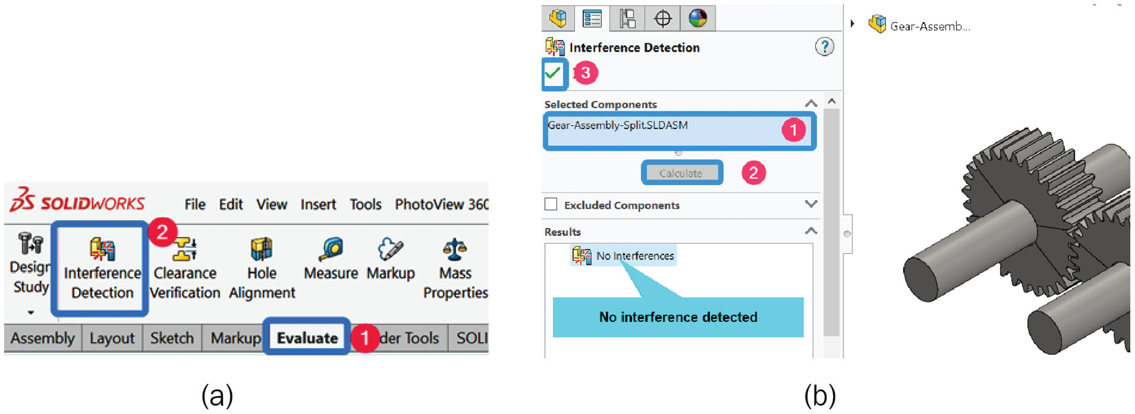
Figure 6.33 – Checking interference
- Next, click on the Calculate button, labeled 2 in Figure 6.33b (notice that this will be grayed out after you click it). The outcome of the interference calculation will be revealed in the Results box.
- Click OK.
As you can see in Figure 6.33b, there is no interference in the assembly. Therefore, we will move to the simulation phase.
Creating the simulation study for the gear and simplifying the assembly
For this purpose, follow the steps given next:
- Using the Simulation tab, launch a New Study.
- From the Study property manager that opens, provide a name for the study, for example, Gear analysis.
- Click OK.
After completing steps 1–3, the simulation environment is launched. You will then notice the four bodies contained in the assembly, as shown in Figure 6.34a. For this analysis, we are interested in the gears. Since the shafts are not of interest for this simulation, they will be removed using one of the useful features of the simulation environment (Exclude from Analysis).
To achieve the exclusion of the shafts from the analysis, carry out the following steps:
- Select the two shafts and right-click within the selected region, as shown in Figure 6.34b.
- From the menu that appears, choose Exclude from Analysis.
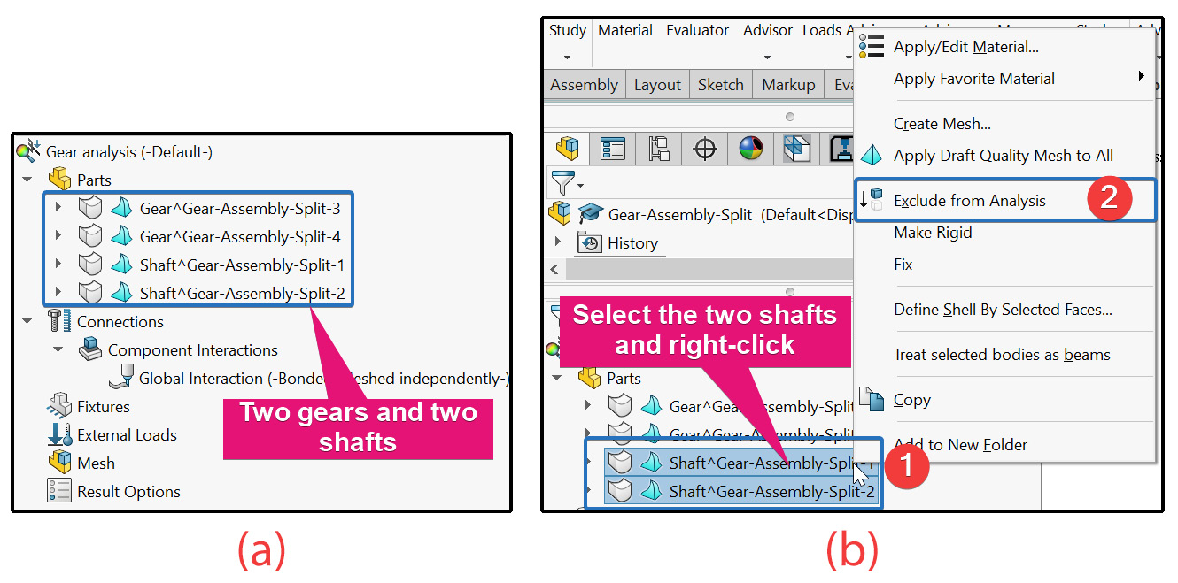
Figure 6.34 – (a) Four bodies in the assembly; (b) excluding the shafts from the analysis
The preceding steps will smartly prevent the two shafts from being considered in our analysis. This has the advantage of reducing the size of the components that will be meshed and the duration of our analysis. You won't always have to do this, but it is a useful tool to be aware of.
Having achieved the removal of the shafts, our next task is to apply materials.
Assigning materials to the gears
The material for the gears is plain carbon steel. Specify the material by following the steps given next to assign the material to the three bodies at once:
- Right-click on the two gears and choose Apply/Edit Material (Figure 6.35).
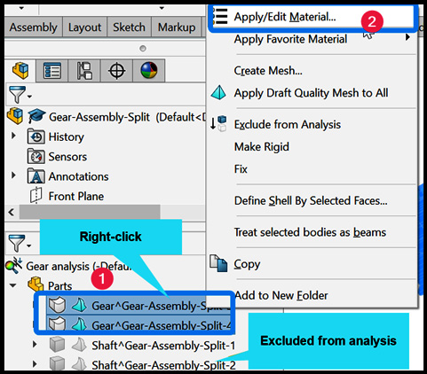
Figure 6.35 – Specifying the material for the gears
- From the materials database that appears, expand the Steel folder.
- Click on Plain Carbon Steel.
- Click Apply and Close.
Our next task is setting up the interaction condition. This is crucial for getting a realistic result for the gear analysis.
Setting up the interaction condition for the gears
As mentioned in the sub-section Examining the interaction setting (for case study 1), the default behavior of SOLIDWORKS is to define a bonded interaction for bodies/components that are in contact. Now, since the gears will be in contact but not bonded, for this case study, the interaction condition needs to be modified.
To set up the right contact, carry out the following steps:
- Expand the Connections folder and then delete the Global Interaction (Figure 6.36).
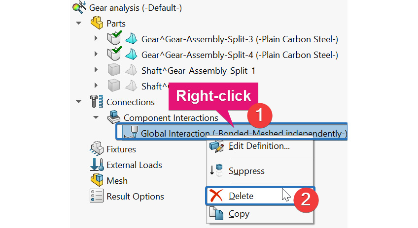
Figure 6.36 – Deleting the bonded contact set
- Next, right-click on the Connections folder again and choose Local Interactions.
This launches the Local Interactions manager, inside which we take the steps that come next.
- Within the Local Interactions window, under Interaction, select Manually select local interactions (labeled 1 in Figure 6.37).
- Under Type, select Contact (labeled 2 in Figure 6.37).

Figure 6.37 – Setting up a local contact interaction
- Under the box for Set 1 (labeled 3 in Figure 6.37), navigate to the graphics window and click on the contacting faces in the split zone of gear A.
- Under the box for Set 2 (labeled 4), navigate to the graphics window and click on the contacting faces on gear B (they should be opposite those of gear A).
- Under Advanced, keep the option as Surface to surface (labeled 5).
- Click OK.
Completing steps 1–8 facilitates the right condition for the interaction between the gears. A bonded interaction, on the other hand, will create a wrong interaction condition between the gears since it will treat the faces as if they were welded together. We are now ready to shift our focus to the fixture.
Applying the fixture to the gears
Each of the two gears needs to be properly supported to behave the way we want. We will specify that gear B is fixed, while gear A can rotate around the Z-axis (based on the problem statement).
The steps to apply the condition for gear B go like this:
- Right-click on Fixtures.
- Pick Fixed Geometry from the context menu that appears.
- When the Fixture property manager appears, navigate to the graphics window and click on the inner face of gear A, as shown in Figure 6.38.
- Click OK.

Figure 6.38 – Defining the fixed fixture
We will now carry out the steps to apply the right boundary condition for gear A:
- Right-click on Fixtures.
- Pick Advanced Fixtures from the context menu that appears.
- When the Fixture property manager appears, click the On Cylindrical Faces option (labeled 1), then navigate to the graphics window and click on the inner face of gear A, as shown in Figure 6.39.
- Under Translations, specify the translation options as shown in the boxes labeled 3–5.
- Click OK.

Figure 6.39 – Options for the advanced fixture on gear A
Notice that for the circumferential rotation (labeled 4 in Figure 6.39), we have entered the value 0.02 radian. This is equivalent to the value of 1.15 degrees specified in the problem statement.
With the completion of the applications of the boundary conditions, we are ready for the meshing phase, which is explored in the next sub-section.
The meshing of the gears
For the meshing operation, we will first create a base mesh (using the curvature-based mesh) and then we will refine the mesh in the contact region. To achieve our aim, take the following steps:
- Right-click on Mesh and then select Create Mesh.
Complete the options as indicated in Figure 6.40a. Notice that we are using the curvature-based mesh. The meshed gears are shown in Figure 6.40b:
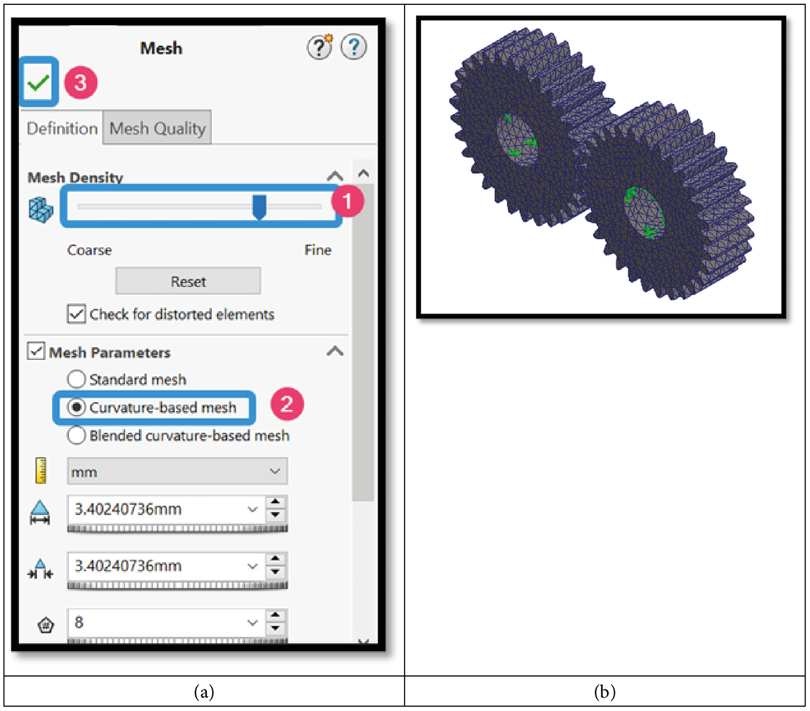
Figure 6.40 – (a) Options to select the curvature-based mesh; (b) the meshed solid gears
The mesh created in step 1 is applied to the whole body of the two gears. To have a more refined mesh around the contact region, we will deploy the Mesh Control command as follows.
- Right-click again on the Mesh folder in the simulation study tree and then select Apply Mesh Control (Figure 6.41a).
- When the Mesh Control property manager appears, under Selected Entities, click inside the reference entities box (labeled 1). Navigate to the graphics window and click on the split faces as shown in Figure 6.41b.
- Drag the Mesh Density slider (labeled 3) to the rightmost end (fine density).
- Click on Create Mesh.
- Click OK.

Figure 6.41 – Mesh control for the contact regions
The difference between the area we have applied mesh control to and the other areas of the gears can be seen in Figure 6.42:
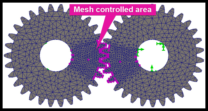
Figure 6.42 – Refined mesh in the contact zone
You can check the mesh details to examine the quality of the mesh (as we did in the previous sub-section Examining standard and curvature-based meshes). As seen in Figure 6.43, the mesh quality is satisfactory. We have a Maximum Aspect Ratio of around 9. Further, we also see evidence that we are indeed using a set of solid elements (a total number of 44225).
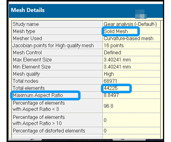
Figure 6.43 – Examining the mesh details for the gears
Now that we have gotten the meshing out of the way and conducted an examination of the generated mesh, let's run and retrieve the results.
Running and obtaining the results
As you know, once the other sub-sections are all properly set up, running the analysis is done in a single step. That is, right-click on the study name (Gear analysis) and then select Run, as shown in Figure 6.44:
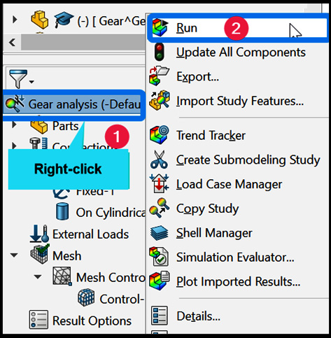
Figure 6.44 – Running the gear assembly analysis
Once the running of the simulation is complete, we will have the set of default results as usual. Indeed, Figure 6.45 depicts the plot of the von Mises stress from among the default results. From the figure, you will notice that a large portion of the two gears experience almost negligible stress from the applied load (mostly blue). However, the contact region is highly stressed.
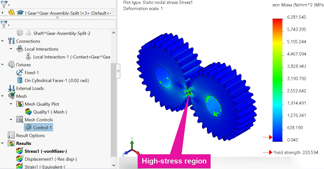
Figure 6.45 – Distribution of the von Mises stress
The design of gears to prevent excessive stress as shown in Figure 6.45 is a specialized topic that is covered over several chapters in textbooks on the design of machine elements. Our interest in this simulation is to confirm two points [4]:
- The largest contact stress will happen at the mating surface of the teeth.
- The largest bending stress will take place at the root of the teeth in contact due to stress concentration.
We'll move on to investigate the stress at the contact region qualitatively. To confirm the first point, carry out the following steps:
- Right-click on the Results folder and then select Define Stress Plot.
Next, adjust the options within the Stress plot property manager that appears as follows:
- Under the Definition tab, below the Display option, select Contact Pressure (Figure 6.46a).
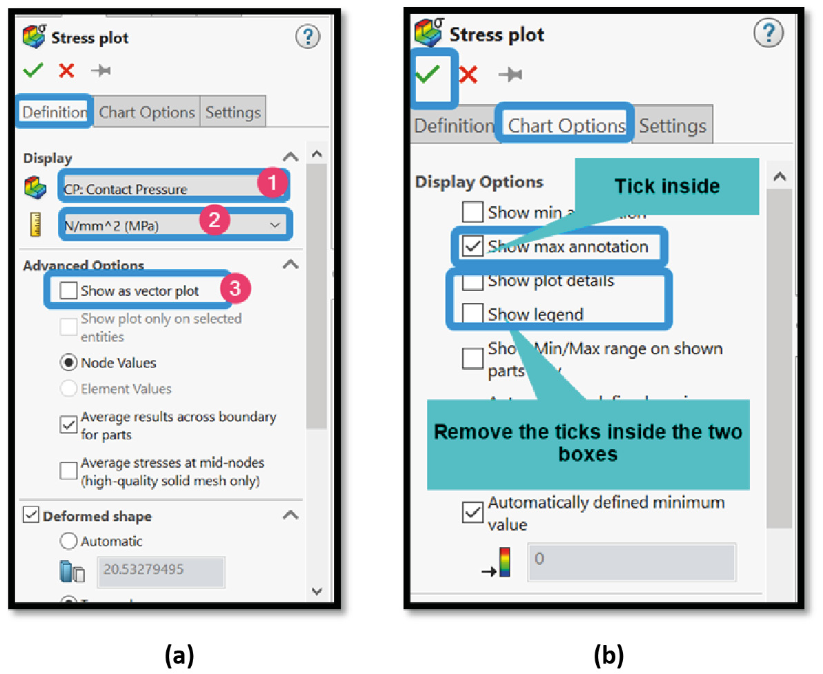
Figure 6.46 – Options for the contact stress
- Under the Definition tab, within the unit box, change the unit to N/mm^2 (MPa)
- Under the Definition tab, below Advanced Options, remove the checkmark inside the box labeled 3 in Figure 6.46a (Show as vector plot).
- Under the Chart Options tab, select the options as shown in Figure 6.46b.
- Click OK.
Once steps 1–6 are complete, the environment is updated with the plot of the contact stress as indicated in Figure 6.47:
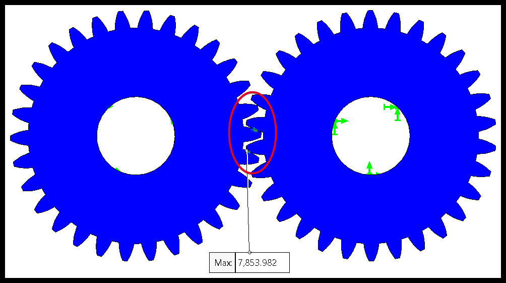
Figure 6.47 – Visualization of the position of the maximum contact stress
Now, if, in step 4 of the preceding steps 1–6, you did not remove the checkmark inside the box, the plot will be as presented in Figure 6.48:

Figure 6.48 – Visualization of the contact stress as a vector plot
Both visualizations in Figure 6.47 and Figure 6.48 confirm that the maximum contact stress indeed happens at the mating surface.
The last result we will look at is the first principal stress. We are using the principal stress as a proxy for bending stress. For this purpose, take the steps outlined next to obtain the principal stress:
- Right-click on the Results folder and then select Define Stress Plot.
- Within the Stress plot property manager, under the Definition tab, navigate to Display and select P1: 1st Principal Stress (Figure 6.49a).

Figure 6.49 – Options for the contact stress
- Under the Definition tab, within the unit box, change the unit to N/mm^2 (MPa).
- Under the Definition tab, below Advanced Options, check the box labeled 3 in Figure 6.49a (Element Values).
- Under the Chart Options tab, select the options as shown in Figure 6.49b.
- Click OK.
With the completion of steps 1–6, the environment is again updated with the plot of the principal stress, as shown in Figure 6.50:
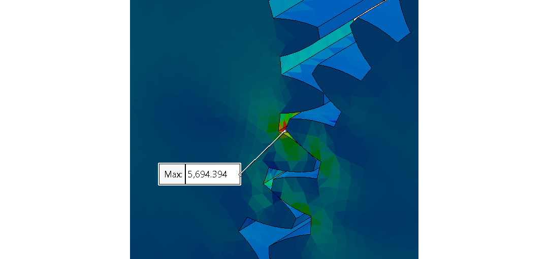
Figure 6.50 – Visualization of the first principal stress at the root of the teeth
Again, it can be seen from Figure 6.50 that the maximum bending stress indeed happens at the root of the tooth that experiences the maximum contact stress. We have only focused on qualitative assessments in the last two results to bring home the concepts. For some other variations of this case study, the numerical values of the stress need to be checked for failure analysis and so on. Besides, it is also possible to employ symmetry for the gear problem (for instance, by using a quarter of each gear). We can also do further mesh refinement and so on.
This wraps up our exploration of the two case studies. Over the course of the two case studies, we've explored some additional features of SOLIDWORKS Simulation. For instance, we demonstrated the following:
- How to employ curvature-based meshes for highly curved members
- How to simplify solid bodies for analysis with the Exclude from Analysis command
- How to examine mesh details to confirm the quality
- How to employ mesh control to refine some selected regions of components
- How to set up a contact interaction relationship
- How to obtain and visualize contact pressure/stress
All these concepts are valuable for the simulation of many other types of components and you can extend the idea further in your various design tasks.
Summary
This chapter set out to explore the use of solid elements. It began with an overview of components that are suitable to be analyzed with solid elements and then shifted gear to the analysis of two case studies. The first case study focused on a spring sub-assembly. This was then followed by the second case study on the static analysis of a gear sub-assembly. Along the way, we leveraged on many features of SOLIDWORKS Simulation that are useful for the analysis of moderately complex entities using solid elements.
Up to now, we have dealt with the analysis of components using a single family of elements in each of Chapters 2, Analyses of Bars and Trusses – Chapter 6, Analyses of Components with Solid Elements. In the next chapter, you will learn about analyzing components with mixed elements.
Exercises
- A variable pitch spring is to be made from a music (ASTM A228) wire with a diameter of 20 mm and other data as shown here:
Total number of active coils = 10
Number of inactive coils = 4
Free length = 500 mm
Outside diameter = 120 mm
The spring is ground at the ends. Compute the deflection experienced by the spring when a force of 300 N is applied at its top.
- Repeat case study 2 for cases where: (a) the friction coefficient is set to 0.02 by evaluating the effect of the change of the coefficient of friction on the stress values; and (b) the default bonded interaction is retained with no manual definition of the "contact" interaction. How does this affect the stress distribution?
Further reading
- [1] Fundamentals of Finite Element Analysis: Linear Finite Element Analysis, I. Koutromanos, John Wiley & Sons, 2018.
- [2] Introduction to the Finite Element Method 4E, J. N. Reddy, McGraw-Hill Education, 2018.
- [3] Finite element analysis of a deployable space structure, D. V. Hutton, Edited by Dr. B. F. Barfield, Professor of Mechanical Engineering, the University of Alabama Tuscaloosa, AL, 1982.
- [4] Machine Elements in Mechanical Design, R. L. Mott, Pearson/Prentice Hall, 2004.
- [5] Mechanical springs. Penton Publishing Company, A. M. Wahl, 1944.
- [6] Introduction to Solid Modeling Using SolidWorks 2009, W. Howard and J. Musto, McGraw-Hill Companies Incorporated, 2009.
- [7] Space Modeling with SolidWorks and NX, J. Duhovnik, I. Demsar, and P. Drešar, Springer International Publishing, 2014.