
Excel Services features overview
Collecting data through data models
Creating reports and scorecards
IN the previous chapter, you learned about the administration side of planning for business intelligence (BI) and key performance indicators (KPIs) for your Microsoft SharePoint 2013 environment. Now that you have your environment ready for BI, you can focus on using the BI features of SharePoint. This chapter focuses on the steps to implement better BI solutions using the features and capabilities of Microsoft Excel 2013, Excel Services, and Microsoft SQL Server 2012. You will learn about the different data sources you can use in Excel 2013 and Excel Services, along with how to use the new features in Excel Services, including Excel Services data connections, and creating reports and scorecards using PowerPivot, PivotTables, and Power View. Finally, this chapter looks at the enhanced Excel Services technologies for developers in SharePoint 2013.
Excel BI provides the capability to explore and analyze data of any size and integrate and show interactive representations of the data. In SharePoint 2013, Excel BI offers the following new features:
External data connections. As mentioned in the previous chapter, most external data connections are supported in Excel Services. This includes SQL Server Analysis Services (SSAS), SQL Server databases, OLE DB, and ODBC data sources.
Data models. Data models are supported, so long as an instance of SSAS is registered in Excel Services.
Reports and scorecards. Reports, dashboards, and scorecards created in Excel are supported in Excel Services. PivotTable reports can be viewed, sorted, filtered, and interacted with in the browser through SharePoint. This includes views created by Power View.
Field List and Field Well (PivotChart and PivotTable reports). Opening and using Field List and Field Well are supported through the browser in Excel Services.
Timeline controls. Timeline controls are supported in Excel Services. Before an existing timeline control in Excel Services can be used, the timeline control must be added to a workbook through the Excel client.
Slicers. Slicers are supported in Excel Services, but they must be added to a workbook through the Excel client.
Quick Explore. Quick Explore is supported and is used to browse up and down to view higher or lower levels of information; however, new views cannot be created using Quick Explore through the browser.
Calculated measures and calculated fields. Calculated fields and calculated measures are supported in Excel Services; however, they must be created from the Excel client.
Excel Services, introduced in Microsoft Office SharePoint Server (MOSS) 2007, is a BI tool that allows the sharing of data-connected workbooks and is used primarily for BI scenarios. In SharePoint 2013, Excel Services is a shared service and is only available in the Enterprise edition of SharePoint. Excel 2013 workbooks can be connected to external data sources and then published to a SharePoint library so that the workbooks can be rendered through the browser. The workbook is rendered through the browser via Excel Services and the external data connection is maintained and the data is refreshed when necessary. The published workbooks allow broad sharing of reports through the organization and can be managed and secured according to the organization’s needs.
Excel Services consists of:
Excel Calculation services. Used to load, calculate, call custom code (user-defined), and refresh the data.
Excel Web Access Web Part. Used to display Excel workbooks through the browser.
Excel Web services. Used for programmatic access.
Note
The tutorials in this chapter use the AdventureWorksDW2012 database and AdventureWorksDW2012Multidimensional-EE OLAP cube, which are available at http://msftdbprodsamples.codeplex.com/releases/view/55330. The instructions, “Configure AdventureWorks for Business Intelligence Solutions,” are available at http://technet.microsoft.com/en-us/library/jj573016.aspx.
SQL Server Data Tools are required to perform the steps in this chapter. The SQL Server Data Tools can be downloaded from http://msdn.microsoft.com/en-us/data/hh297027 and installed separately, instead of using the SQL 2012 DVD install.
External data connections are used by Excel to connect to various data sources, and many of the data connections used are supported in Excel Services. As mentioned briefly in Chapter 14 the connections supported by Excel Services include SQL Server, SSAS, and custom OLE/ODBC data providers. The external data connection must be created from the Excel client first and then the Office Data Connection (ODC) file can be uploaded into a trusted data connection library in SharePoint. Data connections stored in a trusted data connection library provide reusability so users can create multiple reports and workbooks using the available data connections. When the data connections are updated, the reports and workbooks using these connections are updated with the current information.
Before a data model can be created, the authentication settings need to be determined and configured. This section details the various authentication methods for Excel Services in preparation for the creation of the ODC file from the Excel client. The different authentication settings that are available when creating the ODC file from the Excel client are listed in Table 15-1.
Table 15-1. Excel Services authentication settings options
Authentication setting | Details |
Use a stored account | Use when Excel Services is configured for authenticating through the Secure Store Service. The user name and password are retrieved from a target application in the Secure Store Service, which then performs a Windows logon. |
None | Use when Excel Services is configured to use the Unattended Service Account. This setting is similar to using a stored account except that Excel Services uses the target application registered under the Unattended Service Account. |
To move forward with the Use A Stored Account option, an account must be granted access to the data source for use with the Excel workbook. This account can be a SQL Server logon, an Active Directory account, or another set of credentials, as required by the data source. This account will be stored in the Secure Store. In this tutorial, an Active Directory account is being used. Once the data access has been established for the account, the next step is to create a SQL Server logon using the Active Directory account for data access.
Follow these steps to grant access in SQL Server:
Open Microsoft SQL Management Studio and connect to the database server that contains the AdventureWorksDW2012 database.
From the Object Explorer, expand Security | Logins.
If your account is not already in the list, continue to step 3.
Right-click Logins and select New Login.
Type in the Active Directory account name for the Login Name or click Search to find the user account. Leave the Windows Authentication option selected.
Select User Mapping, located under the Select A Page option, and then check the Map box for the database you want to provide access to. For this example, select the AdventureWorksDW2012 database, as shown in the following graphic.
Check db_datareader in the Database Role Membership options and then click OK.
Note
Once the account is added, it will show up in the list in the Logins section. Even though the db_datareader option was selected when the setting was created, it may not have been set properly. It is recommended to check the User Mapping for the newly added account to verify that the property is set.
From the Logins section, double-click the account that was just added to reopen the properties.
Click User Mapping, then click AdventureWorksDW2012 under the Database column to make the options active for that database.
If the option is not set, click the db_datareader check box, then click OK.

EffectiveUserName is an SSAS connection string property that allows a per-user identity without the need to configure Kerberos delegation. This property passes the value of the user to SSAS, which is accessing the report or dashboard in Excel Services or PerformancePoint Services.
To use EffectiveUserName, the following parameters are required:
The Excel Service application pool account must be an SSAS administrator.
The EffectiveUserName option must be enabled in the Excel Services Global Settings.
The Use The Authenticated User’s Account option must be enabled in the Excel Services Authentication Settings in Excel.
If this is the preferred authentication method, follow these steps to enable EffectiveUserName in Excel Services:
From Central Administration, click Managed Service Applications, located in the Application Management section, and then click the Excel Services service application that you want to configure.
Click Global Settings.
In the Excel Data section, click the Use The EffectiveUserName Property check box, and then click OK.
This section provides the steps to use the Secure Store in SharePoint to store SQL Server credentials for use with Excel Services or Visio Services. It is recommended to store credentials in Secure Store over storing them in an Excel workbook file or an ODC file because credentials in Secure Store are not stored in plain text. By storing the credentials in the Secure Store, you provide a central location that is easier to manage and update than credentials stored directly in workbook or ODC files.
The following parameters are required in order to use Secure Store with Excel Services or Visio Services to access data sources through SQL Server authentication:
A Secure Store target application containing SQL Server credentials with access to the data source must be configured.
The Unattended Service Account must be configured.
In previous steps in this chapter, the data access account was granted access to the SQL Server database and was given db_datareader permissions. The next step is to create the Secure Store target application.
Creating a target application for SQL Server authentication Follow these steps to create a target application for SQL Server authentication:
From Central Administration, click Managed Service Applications, located in the Application Management section, and then click the SSS service application that you want to configure.
On the ribbon, click New, and then fill in the following in the Create New Secure Store Target Application window:
Target Application ID: Type a unique identifier for this target application. For example, this tutorial uses ExcelServicesSQLAccount.
Display Name: Type a friendly name or short description.
Contact E-mail: Type the email address for the contact used for this target application.
For Target Application Type, select Group from the drop-down list, as shown here.
The two Target Application Type options are:
Click Next to move to the Credentials Fields page.
Leave the default credential fields if you are using Windows credentials. If you are using other credentials, change the Field Type drop-down menus to the appropriate credentials that you are using.
Click Next to go to the Specify The Membership Settings page and enter the following, as shown next.
Target Application Administrators: Type in the account of the user who will be the administrator of this target application. In this example, the default administrator account will be added.
Members: Type the users to whom you want to grant the ability to refresh the data. To give access to all users, type Everyone.
Click OK.


Setting credentials for the SQL Server authentication target application To set the credentials for the Secure Store Target Application, follow these steps:
From the SSS service application management page, select the check box next to the newly created Target Application ID and select Set Credentials on the ribbon.
Set the Windows User Name, Windows Password, and Confirm Windows Password of the data access account, as shown here, and then click OK.

Creating a target application for the Unattended Service Account Use the following steps to create a target application for the Unattended Service Account. If you currently have an Unattended Service Account configured, then the following steps can be skipped.
Note
To determine if an Unattended Service Account has been configured, check the External Data settings in the Excel Services Global Settings.
From Central Administration, click Managed Service Applications, located in the Application Management section, and then click the SSS service application that you want to configure.
On the ribbon, click New, and then fill in the following:
Target Application ID: Type a unique identifier for this target application. For example, this tutorial uses ExcelServicesUnattendedAccount.
Display Name: Type a friendly name or short description.
Contact E-mail: Type the email address for the contact used for this target application.
Target Application Type: Select Group from the drop-down list.
Click Next to move to the Specify Credentials Fields page.
Leave the default credential fields if you are using Windows credentials. If you are using other credentials, change the Field Type drop-downs to the appropriate credentials that you are using.
Click Next to go to the Specify The Membership Settings page and enter the following:
Target Application Administrators: Type in the account of the user who will be the administrator of this target application. In this example, the default administrator account will be added.
Members: Type the users to whom you want to grant the ability to refresh the data. To give access to all users, type Everyone.
Click OK.
Setting credentials for the Unattended Service Account target application To set the credentials for the Unattended Service Account target application, follow these steps:
From the SSS service application management page, select the check box next to the newly created Target Application ID and select Set Credentials on the ribbon.
Set the Windows User Name, Windows Password, and Confirm Windows Password of the data access account and then click OK.
Configuring the Unattended Service Account To configure the Unattended Service Account for the Secure Store Target Application, follow these steps:
From Central Administration, click Managed Service Applications, located in the Application Management section, and then click the Excel Services service application that you want to configure.
Click Global Settings.
From the External Data section, select the Use An Existing Unattended Service Account option, and in the Target Application ID text box, input the name of the target application that you created for the Unattended Service Account, as shown here.
Click OK.

This section covers the steps to configure Secure Store settings in Excel using the AdventureWorksDW2012 sample database and sample tables.
To configure the Secure Store settings in Excel, follow these steps:
Open Excel 2013 and click Blank Workbook to create a new workbook or open an existing workbook.
Click the Data tab, and in the Get External Data group, click From Other Sources | From SQL Server, as shown here.
In the Data Connection Wizard, input the name of the server where the AdventureWorks data resides in the Server name box.
Select the Log On credentials according to your organization based on the following:
For Windows Authentication, choose Use Windows Authentication and click Next.
For specific user credentials, choose Use The Following User Name And Password, input the appropriate credentials and click Next.
From the Select The Database That Contains The Data That You Want list, select the AdventureWorksDW2012 database.
Select both the Connect To A Specific Table and the Enable Selection Of Multiple Tables check boxes.
Select the check box for each of the following database tables:
DimProduct
DimPromotion
DimSalesTerritory
FactInternetSales
FactResellerSales
Verify that Import Relationships Between Selected Tables is selected, as shown here, and click Next.
Optional: Change the File Name, input a Description, and modify the Friendly Name to the desired settings, as shown here.
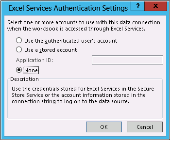
Click Authentication Settings. Select None, as shown here, and then click OK.
The entire options available are as follows:
Select Use The Authenticated User’s Account if Excel Services is using Claims to Windows Token Service.
Select Use A Stored Account if Excel Services is configured to use SSS.
Select None if Excel Services is configured to use the Unattended Service Account.
Note
See Table 15-1 for more details on authentication setting options.
Click the Browse button next to the File Name text box. Note the location where the data source is being saved or change the location.
Click Save, and then click Finish.
From the Import Data dialog box, click Only Create Connection and then click OK.


Note
Secure Store is used by Excel Services when the workbook is rendered from a SharePoint site. The Excel client does not use Secure Store and connects to the database directly. Once the workbook is connected to the data source, you can complete changes to the workbook and then publish to a SharePoint site so that it can be rendered with Excel Services. The connection information to the Secure Store target application will remain embedded in the workbook file.
The Secure Store connection information can be exported as an ODC file, which allows easier management and distribution of data connections so it can be used by additional Excel workbooks.
Follow these steps to export the ODC file:
In Excel, click Connections located in the Data tab.
Select the connection that you just created in the previous steps and then click Properties.
Click Definition | Authentication Settings.
Confirm the Use A Stored Account option is selected and the correct Application ID is specified, and then click OK.
Click Export Connection File.
Keep the workbook open.
Before uploading the ODC file to the BI Center trusted data connection library, the next step is to add the data connection library to the Excel Services Trusted Data Connection Libraries settings.
Follow these steps to add the ODC file to the trusted data connection library:
From Central Administration, click Managed Service Applications in the Application Management group, and then click the Excel Services service application that you want to configure.
Click the Trusted Data Connection Libraries link and then click Add Trusted Data Connection Library.
Type in the address of the BI Center site data connection library (for example, http://contoso/sites/bicenter/Data%20Connections) in the Location section and input a Description (optional).
Click OK.
This section provides the steps to upload the ODC file that was created in the previous steps.
To upload an ODC file, follow these steps:

When using Excel to access data, you can create your own data connections or use an existing data connection. When creating new data connections for SharePoint Server 2013, the connection must be created from Excel 2013 first, and then the ODC file can be uploaded into a trusted data connection library in SharePoint and be used to create reports, scorecards, and dashboards. Before the file can be uploaded, Excel Services must be configured to include a trusted data connections library and a trusted documents library. If Excel Services has not been configured, please refer to Chapter 14 to configure Excel Services. When SSAS retrieves the value when the call is being made, SSAS returns the results of the query, which are security-trimmed based on the user.
Follow these steps to use an existing data connection in Excel:
Follow these steps to create a new data connection in Excel:
In Excel, click the Data tab and then pick one of the From Other Sources options that is available in the Get External Data group:
SQL Server
SQL Analysis Services
Windows Azure
OData
XML file
Or data accessed through a custom data provider
Follow the steps of the Data Connection Wizard and specify all required information, and then click Finish.
From the Import Data page, select how you want to view the data and then click OK.
As mentioned in Chapter 14, Excel Services enables the ability to view and use Excel workbooks that have been published to SharePoint. One of the ways to collect data is through data models. A data model is a useful way for gathering a collection of data from a variety of sources that you create and organize by using PowerPivot for Excel. These sources include SQL Server, Microsoft Access, OData feeds, Windows Azure, XML files, and other custom providers. You can sort, organize, and create relationships between different tables in Excel, and once the data is imported and organized into a data model, you can use it as a source for creating powerful reports, scorecards, and dashboards.
The advantages to using data models over connecting to external data sources are as follows:
You can gather data from multiple sources and put it together as a single data set.
Flash Fill functionality is supported to format columns.
You can view, sort, and organize the data.
In SharePoint 2010, data models were queried, but they could not be refreshed interactively. The most significant improvement for PowerPivot in SharePoint 2013 is the ability to refresh data models interactively all the way down from the original data sources. Excel Services in SharePoint 2013 retains the connection to the external data sources so that the data stays updated. Excel Services first sends processing commands to the SSAS that is hosting the data model and then queries the data model to update the workbook. The update is processed when you click the Refresh Selected Connection or Refresh All Connections command from the data menu in the browser for the Excel workbook.
Note
Data models interactive refresh only works for workbooks created in Excel 2013. Excel Services will display an error message if you try to refresh an Excel 2010 workbook.
Two options are available to refresh a data model in Excel Services: interactive and scheduled, which are outlined in Table 15-2.
Table 15-2. Data model refresh options
Refresh option | Details |
Interactive Data Refresh | Available out-of-the-box when a SQL Analysis server is registered in Excel Services. Only refreshes the data in the current user’s session and does not save the data back to the workbook. Can use the identity of the current logged-on user or use stored credentials to connect to the data source. Only works for workbooks created in Excel 2013. |
Scheduled Data Refresh | Requires the deployment of the PowerPivot add-in for SharePoint. Opens workbook in a separate refresh session and saves the updated version back to the content database. Uses stored credentials. Works for workbooks created using SQL Server 2012 PowerPivot add-in for Excel 2010 or workbooks created in Excel 2013. |
In Excel 2013, much of the functionality from Excel 2010 to import and relate large amounts of data from multiple sources is built directly into the data model. Without installing a separate add-in, you can do the following:
Import millions of rows from multiple data sources.
Create relationships between data from different sources and between multiple PivotTable tables.
Create implicit calculated fields (previously called measures).
Manage data connections.
Now data models can be used as the basis for PivotTables, PivotCharts, and Power View reports. Excel automatically loads the data into the xVelocity in-memory analytics engine, which used to be available only with the PowerPivot add-in.
SharePoint 2013 provides the ability to create powerful reports and scorecards for data analysis. This section provides the functionality for PowerPivot and Power View to create dynamic reports and scorecards for your BI Center.
You may or may not be familiar with PowerPivot. What is PowerPivot? PowerPivot for Excel is an add-in used to perform powerful data analysis that extends the capabilities of PivotTable data summarization and cross-tabulation by having the ability to import data from multiple sources. PowerPivot provides a richer modeling environment allowing more experienced users to enhance their data models. The add-in was available for download for Excel 2010 and is built into Excel 2013 in Microsoft Office Professional Plus. Although this add-in is built into Excel 2013, it is not enabled by default; therefore, it will need to be enabled in order to use this feature.
Even though PowerPivot was available in SharePoint 2010, most organizations did not use nor implement the feature. Organizations wanted reporting features, but the implementation and SQL Server requirements for PowerPivot were different than they are now for SharePoint 2013. SQL Server had Excel add-ins for building data models in Excel 2010 and were not part of an internal SharePoint feature.
In SharePoint 2013, there has been a paradigm shift in that Excel 2013 and Excel Services now fully integrate data models as an internal feature. The new architecture for SQL Server 2012 SP1 PowerPivot supports the ability to have a PowerPivot server outside of a SharePoint 2013 farm. Even though it is not required, the PowerPivot server can still be installed on a SharePoint server. Excel Services in SharePoint 2013 includes data model functionality to enable interaction with PowerPivot workbooks through the browser without the need to deploy the PowerPivot for SharePoint add-in to the farm. However, this add-in does provide additional functionality and features to your SharePoint farm.
Deploying the PowerPivot for SharePoint 2013 add-in enables the following additional features:
PowerPivot Gallery
Schedule Data Refresh
PowerPivot Management Dashboard
Note
The PowerPivot for SharePoint 2013 add-in is available for download at http://www.microsoft.com/en-us/download/details.aspx?id=35577.
This section reviews the PowerPivot features available in SharePoint 2013 that are supported in Excel Services.
Filters and timeline Excel and PowerPivot both allow data to be imported, and PowerPivot provides the ability to filter out unnecessary data for the import. The timeline control, shown on the ribbon in Figure 15-1, is a new time filter that makes it easier to compare PivotTable and PivotChart data over different time periods. Instead of grouping by dates, you can create a PivotTable timeline to filter dates interactively or to move through data in sequential time periods.

Figure 15-2 shows a sample workbook that includes a slicer and a timeline control. When the user clicks a value on the slicer or the timeline, the PivotTables update accordingly.

Field List and Field Well support Excel Services enables the ability to open the Field List and Field Well for PivotChart and PivotTable reports through the browser, as shown in Figure 15-3. This added capability makes it easy to change the displayed information temporarily in a PivotChart or PivotTable report without having to open the Excel client.

Figure 15-3. With Excel Services, the Field List and Field Well for PivotChart and PivotTable reports can be opened through the browser.
If you are not using the Excel Access Web Part to render the workbook, the Field List and Field Well can be disabled through the Excel client. Once it is saved into the document library, the Field List will no longer show up. To re-enable the Field List, make the update on the ribbon in the Excel client, as shown in Figure 15-4, and then save it back to the document library.

If you are using the Excel Access Web Part to render the workbook, the PivotTable and PivotChart Modification property can be set on the web part, as shown in Figure 15-5.

Renaming tables and columns As data is imported through PowerPivot, tables and columns can be renamed.
Diagram view When working with data models that contain a lot of tables, it is sometimes easier to work with the tables through Diagram view (see Figure 15-6). Diagram view is an Excel 2013 PowerPivot add-in that allows you to manage the data models. Diagram view also provides a great way to help understand your entire data model by being able to see what fields are related between tables. You can also use the drag-and-drop feature to create new relationships in the Diagram view.
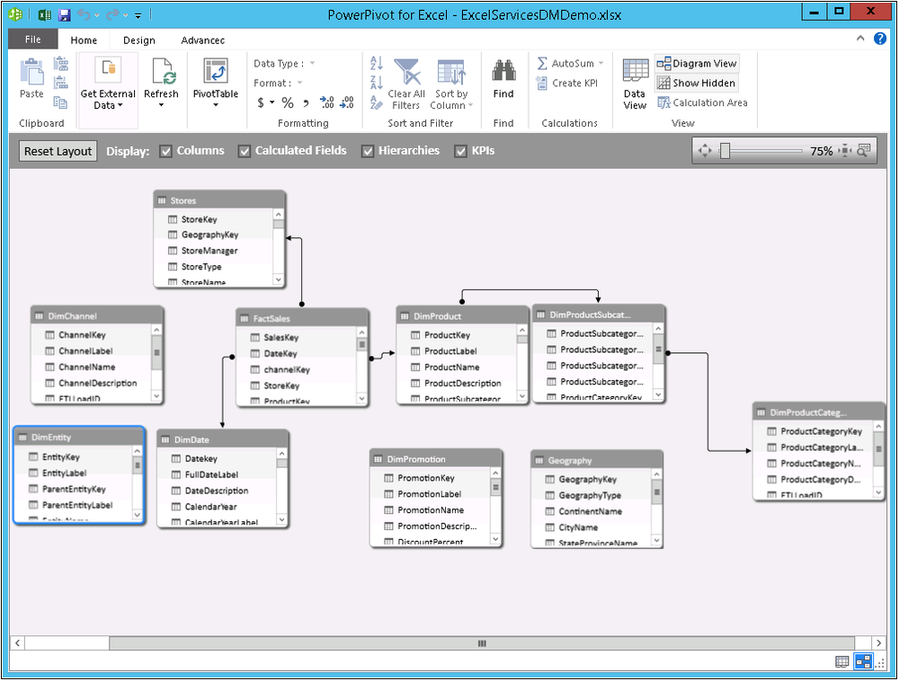
Figure 15-6. An example of a Diagram view in Excel 2013 displayed through the PowerPivot for Excel window.
Formatting You can apply various types of formatting to Power View and PowerPivot reports. This includes styling of the workbook, charts, and other elements.
Calculated fields Calculated fields, previously known as measures, are calculations used in data analysis, such as sums, counts, averages, and minimum/maximum values. Excel Services supports the ability to define custom calculated fields, as shown in Figure 15-7.

Key performance indicators KPIs, in essence, are quantifiable measurements for gauging business objectives. A KPI in PowerPivot is based on a specific calculated field designed to help evaluate current value and current status of a metric against a defined target. KPIs can be defined and used in PivotTables.
KPIs are covered in Chapter 16.
Perspectives Perspectives in PowerPivot are custom views that can be defined for a particular business scenario or user group that make it easier for users to navigate through large data sets. Perspectives can include any combination of tables, columns, KPIs, and multiple perspectives can be created.
Advanced formulas Author custom calculations by writing advanced formulas that use the Data Analysis Expressions (DAX) expression language.
Before we can begin to work with PowerPivot, we need to enable PowerPivot for Excel and SharePoint. To enable PowerPivot in Excel 2013, follow these steps:
In Excel, go to File | Options | Add-Ins.
In the Manage drop-down, select COM Add-ins, and then click Go.
Click the Microsoft Office PowerPivot for Excel 2013 check box and then click OK.
Click the PowerPivot tab get to the PowerPivot options, as shown next.
To open the PowerPivot window, click Manage.

Figure 15-8, Figure 15-9, Figure 15-10, Figure 15-11, and Figure 15-12 display the PowerPivot window and tab options for a workbook that was created using the existing data connection from the section “Configuring Secure Store settings in Excel” earlier in this chapter.


Figure 15-9. The PowerPivot window Home tab options display the available options in the drop-down menu for the PivotTable command.

Figure 15-10. The PowerPivot window Home tab options display the available drop-down menu items for Get External Data.


Because this workbook is already connected to an existing data connection, it displays the imported data with a tab at the bottom for each table that is part of the data connection query. The PowerPivot options for this data can be updated accordingly (Figure 15-11), and then a PivotTable of choice can be generated by using the PivotTable ribbon button, or you can connect to more data sources by using the Get External Data ribbon button shown in Figure 15-12.
If you created a new workbook without importing data, the PowerPivot window opens displaying a blank worksheet, as shown in Figure 15-13. A PivotTable cannot be created until data is imported using the Get External Data ribbon button.

Before working with PowerPivot, the PowerPivot Feature Integration for Site Collections feature must be activated. To enable PowerPivot in SharePoint, follow these steps:

Once the PowerPivot Feature Integration for Site Collections feature is activated on the site collection, the PowerPivot Gallery becomes available in the list of available apps.
Follow these steps to create a PowerPivot Gallery library:
From the BI Center site, click the Site Settings icon | Site contents.
Click Add An App, and then click the PowerPivot Gallery tile.
Click Advanced to go to the advanced settings creation page.
Set the following:
Name: Type a friendly name for your library, or use PowerPivotDocuments.
Description: Type a description. (This setting is optional).
Document Version History: Default value is No; however, change to Yes if you want versioning turned on for this document library.
Document Template: Set the drop-down value to Microsoft Excel Spreadsheet.
Click Create.

This section provides the steps to create a basic sales dashboard that contains several reports using an external data connection pulling from SSAS data.
In order to create a dashboard from Excel, a data connection must be created first, as follows:
Open Excel 2013 and choose Blank Workbook.
From the Data tab, choose From Other Sources (located in the Get External Data group) and then select From Analysis Services.
In the Connect To Database Server step, specify the name of the server where the Analysis Services data resides.
In the Log On Credentials, choose one of the following:
Use Windows Authentication
Use The Following User Name And Password
From the Select Database And Table dialog box, select AdventureWorksDW2012Multidimensional-EE from the drop-down list.
Select the Adventure Works cube and then click Next.
From the Save Data Connection File And Finish step, shown in the following graphic, update the File Name, Description (optional), and Friendly Name.
Click Authentication Settings, set the authentication to None, and then click OK.
Click Finish.
From the Import Data dialog box, select Only Create Connection, and then click OK.
Keep Excel open and save the workbook locally.
Name the file (for example, Adventure Works Sales) and leave the workbook open.


Now that the data connection has been created, the next step is to create the PivotTable and PivotChart reports. The following dashboard reports will be created:
ProductSales PivotChart report. A bar chart report to show sales amounts across different product categories.
GeoSales PivotChart report. A bar chart report to show sales amounts across different sales territories.
ChannelSales PivotTable report. A table to show order quantities and sales amounts across the Internet and reseller channels.
OrderSales Pivot Table report. A table to show order quantities and sales amounts across different product categories.
Creating a ProductSales PivotChart Follow these steps to create a PivotChart report called ProductSales:
In Excel, select cell A9 and then click the Insert tab. In the Charts section, choose PivotChart.
In the Create PivotChart dialog box, select Use An External Data Source, as shown in the following graphic, and click Choose Connection.
In the Existing Connections wizard, select AdventureWorksDW2012Multidimensional-EE, and then click Open.
In the Create PivotChart dialog box, leave the Existing Worksheet option checked and click OK.
In the Analyze tab, in the Chart Name box (PivotChart group), change the name from Chart1 to ProductSales and press Enter.
From the PivotChart Fields panel, shown here, select the following:
In the Sales Summary section, select Sales Amount.
In the Products section, choose Product Categories.
Next, sort the bars in descending order by following these steps:
From the PivotChart, select the down arrow on the Product Categories control.
In the Select Field dialog box, click More Sort Options.
From the Sort (Category) dialog box, select the Descending (Z to A) By option and set the drop-down value to Sales Amount.
Click OK. The bar graph should now be updated according the sort order, as shown here.
Save the file and leave the workbook open.


Creating a GeoSales PivotChart report Follow these steps to create a PivotChart report called GeoSales:
In the existing workbook, choose an empty cell where you want to add a new PivotChart report, such as G9.
On the Insert tab, choose PivotChart.
In the Create PivotChart dialog box, select Use An External Data Source and click Choose Connection.
In the Existing Connections wizard, select AdventureWorksDW2012Multidimensional-EE, and then click Open.
In the Create PivotChart dialog box, leave the Existing Worksheet option checked and click OK.
On the Analyze tab, in the Chart Name box (PivotChart group), change the name from Chart2 to GeoSales and press Enter.
In the PivotChart Fields panel, shown here, select the following options:
In the Sales Summary section, select Sales Amount.
In the Sales Territory section, drag Sales Territory to the Legend section.
Save the file and leave the workbook open.
Select and move the PivotCharts down to leave some empty cells at the top. The empty cells at the top will be where the Timeline control will be added later in this chapter.
Setting the sizing for the PivotCharts To ensure that the PivotCharts will not have sizing issues, we will specify the size settings for the report. To do this, follow these steps for each of the PivotChart reports:
In an empty section of the PivotChart report, right-click and select Format Chart Area from the select menu.
The Format Chart Area list opens.
Below the Chart Options, choose the Size and Properties icon.
Expand the Size section and check the Lock Aspect Ratio option.
Expand the Properties section and check the Don’t Move Or Size With Cells option.
If you want to specify alternate text for the report, expand the Alt Text section and type the text that you want to use for the report.
Repeat these steps for all PivotCharts. Once complete, close the Format Chart Area panel by clicking the Close button in the panel.
Save the file and leave the workbook open.
Creating a ChannelSales PivotTable report Follow these steps to create a PivotTable report called ChannelSales:
In the existing workbook, choose an empty cell where you want to add a new PivotTable report, such as A25.
On the Insert tab, choose PivotTable.
In the Create PivotTable dialog box, select Use An External Data Source, and click Choose Connection.
In the Existing Connections wizard, select AdventureWorksDW2012Multidimensional-EE, and then click Open.
In the Create PivotTable dialog box, leave the Existing Worksheet option checked and click OK.
On the Analyze tab, in the PivotTable Name box (PivotTable group), change the name from PivotTable3 to ChannelSales and press Enter.
In the PivotTable Fields panel, shown here, select the following:
In the Sales Orders section, select Order Count.
In the Sales Summary section, select Sales Amount.
In the Sales Channel section, select Sales Channel.
In the ChannelSales PivotTable, select the cell that says Row Labels. On the Formula bar at the top for the selected cell, change the text Row Labels to Channel Sales.
Save the file and leave the workbook open.

Creating an OrderSales PivotTable report Follow these steps to create a PivotTable report called OrderSales:
In the existing workbook, choose an empty cell where you want to add a new PivotTable report, such as G25.
On the Insert tab, choose PivotTable.
In the Create PivotTable dialog box, select Use An External Data Source, and click Choose Connection.
In the Existing Connections wizard, select AdventureWorksDW2012Multidimensional-EE, and then click Open.
In the Create PivotTable dialog box, leave the Existing Worksheet option checked and click OK.
On the Analyze tab, in the PivotTable Name box (PivotTable group), change the name from PivotTable4 to OrderSales and press Enter.
In the PivotTable Fields panel, shown in the following graphic, select the following:
In the Sales Orders section, select Order Count.
In the Sales Summary section, select Sales Amount.
In the Product section, select Product Categories.
In the OrderSales PivotTable, select the cell that says Row Labels. On the Formula bar at the top for the selected cell, change the text Row Labels to Products.
Save the file and leave the workbook open.
Creating a Timeline control filter This section provides the details to create a Timeline control to enable the users to filter the data for a particular time.

To create a Timeline control, follow these steps:
In the existing workbook, choose an empty cell where you want to add the Timeline, such as A1.
On the Insert tab, in the Filters section, select Timeline.
In the Existing Connections dialog box, select AdventureWorksDW2012Multidimensional-EE, and then click Open.
Select Date, and then click OK.
Move the Timeline control to a preferred location in the workbook.
To resize, drag the resizing handles on the right side of the control to the desired size.
Select the Timeline control to make it active, and then click the Options tab. In the Timeline group, select Report Connections.
The Report Connections dialog box appears.
Select all four reports (ChannelSales, GeoSales, OrderSales, and ProductSales), and then click OK.
Save the file and leave the workbook open.
Before publishing the workbook, we will make some minor adjustments to it to improve the look and feel of how the dashboard will be displayed in the browser. By default, the dashboard displays gridlines on the worksheet; therefore, we will hide the gridlines to make it look cleaner. We will also rename the worksheet tab from Sheet1 to something else.
To remove the gridlines, select the View tab and clear the Gridlines check box located in the Show section.
To remove row and column headings, clear the Headings check box.
To rename the worksheet tab, right-click Sheet1 and select Rename.
Type a name such as Sales Dashboard, as shown here, and press Enter.
Save the file and leave the workbook open.

The next step is to upload your data connection file and Excel workbook dashboard to your BI Center site.
To upload your data connection file to your BI Center, follow these steps:
Open the BI Center site.
Click Data Connections.
Open Windows Explorer and navigate to your saved AdventureWorksDW2012Multidimensional-EE.odc file.
The location used for this tutorial is C:UsersAdministratorDocumentsMy Data Sources.
Drag the AdventureWorksDW2012Multidimensional-EE.odc file from Windows Explorer to the Drag Files Here section of the Data Connections library on the site.
Now upload your Excel workbook to your trusted documents library used for your Excel Services workbooks. To upload your Excel workbook to your BI Center, follow these steps:
From the BI Center site, click Libraries in the left navigation pane, and then click the PowerPivotGallery tile.
Open Windows Explorer and navigate to your saved workbook file.
The location used for this tutorial is C:UsersAdministratorDocuments.
Drag the Excel file from Windows Explorer to the Drag Files Here section of your Documents library on the site.
Navigate back to the PowerPivotGallery main page to see the graphical list of your newly uploaded workbook, as shown in the following graphic.
Click the newly uploaded file to render the file through the browser using Excel Services, as shown here.
You can browse through, filter, and interact with the data to see the charts change based on your selections.
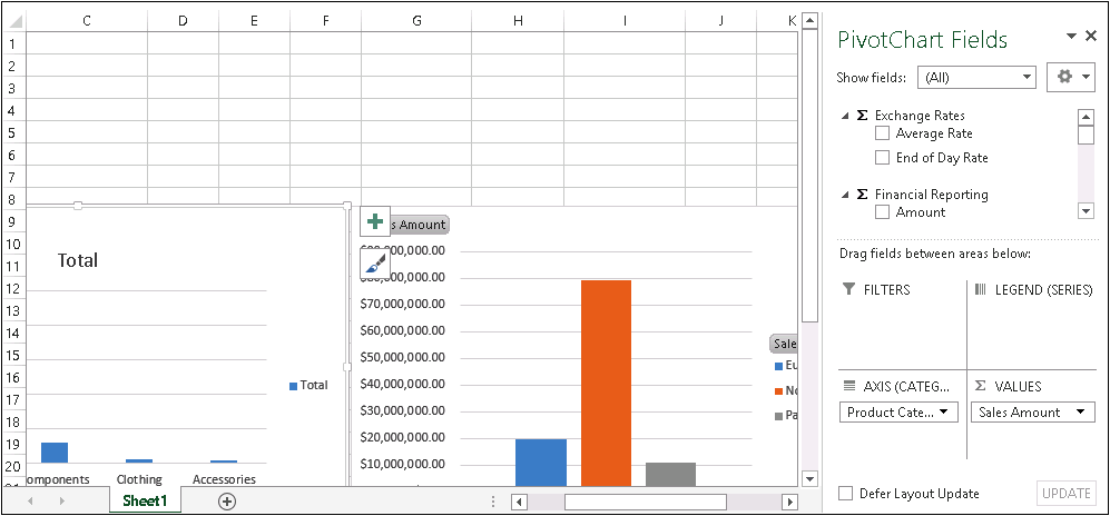
Right-click the PivotTable or PivotCharts and select Show Field List to display the Fields panel.


The previous image displays the PivotChart Fields panel for the workbook that is being displayed through the browser. The Source Currency field was selected, which changed the GeoSales PivotChart dynamically.
Power View is an add-in for Excel 2013 and a SharePoint feature that provides an interactive data exploration, visualization, and presentation experience to create mashups and interactive dashboards that encourages intuitive, ad-hoc reporting. With Power View, you can interact with data in the same Excel workbook as the Power View sheet, in data models in Excel workbooks published to PowerPivot galleries, and in tabular models deployed to SSAS instances.
Note
To use Power View, the SQL Server Reporting Services service application must be configured on the SharePoint farm. The instructions “Install Reporting Services SharePoint Mode for SharePoint 2013” are available at http://msdn.microsoft.com/en-us/library/jj219068.aspx.
Excel 2013 workbooks with Power View sheets can be saved to SharePoint Server 2013 on-premises or SharePoint Online in Office 365. Users can view and interact with the reports; however, the Power View sheets created from the Excel client can be edited only from the Excel client. The interaction in SharePoint includes visualization interactions such as filtering, sorting, highlighting data in charts, and slicers. The reason why Power View sheets cannot be modified directly from SharePoint if the Power View was created through the Excel client is that Power View sheets are part of the XSLX file and Power View reports created from SharePoint are RDLX files, not XLSX files. When creating Power View reports directly from SharePoint instead of the Excel client, the reports are saved directly on the server, where others can view and interact and those who have permissions can also edit the Power View reports.
To enable Power View in Excel 2013, follow these steps:
From Excel, go to File | Options | Add-Ins.
In the Manage drop-down, select COM Add-ins, and then click Go.
Click the Power View check box, and then click OK.
Click the Insert tab, and the Power View button should now be available and enabled, as shown here.
Click Power View to open Power View, as shown in the following graphic.


Note
For more information on Power View, see “Power View: Explore, visualize, and present your data,” located at http://office.microsoft.com/en-us/excel-help/power-view-explore-visualize-and-present-your-data-HA102835634.aspx.
This section provides a high-level overview of the Excel Services additions and enhancements for developers in SharePoint 2013. Excel Interactive view and ECMAScript (JavaScript, Jscript) user-defined functions (UDFs) are two of the new technologies added to Excel Services.
Excel Interactive view is a new technology that uses HTML, JavaScript, and Excel Services to generate table and chart views contemporaneously in the browser from an HTML table hosted on a page. Using Excel Interactive view enables the users to harness the analytical power of Excel for use on any HTML table on a page without having to install Excel.
To enable Excel Interactive view, simply insert two HTML tags on your page in your site. The first tag inserted into the HTML of the page is a standard HTML <a> tag that has attributes that you can configure in Excel Interactive view. You insert the <a> anchor tag above the HTML for the table that has the data you want to use to create the Excel Interactive view, as highlighted in Figure 15-14. Table 15-3 lists the Excel Interactive view tag attributes.

Table 15-3. Excel interactive view tag attributes
Description | Default value | Required? | |
data-xl-dataTableID | Unique identifier for the table. | N/A | No |
data-xl-buttonStyle | Sets the button graphic style. Two style options are standard and small. | Standard | No |
data-xl-fileName | Sets the name of the workbook that the user can download by clicking the Download button in the Excel Interactive view. | “Book1” | No |
data-xl-tableTitle | Sets the title of the table. This attribute can be set to up to 255 characters long. Something to consider when naming the title is that if the table is small but the title is long, the display of the title could be cut off. | Same as the webpage title. | No |
data-xl-attribution | Sets a message used to describe the source for the view that displays within the workbook when viewed. This attribute can be set to up to 255 characters long. | “Data provided by [website domain]” | No |
The second tag that needs to be inserted into the HTML of the page is a standard HTML <SCRIPT> tag that references the JavaScript file that creates the Excel Interactive view. In Figure 15-15, the script is added to the PlaceHolderAdditionalPageHead content placeholder of the page.

Note
To add the tag to a site that uses SSL, change the src attribute to also use https://, such as https://r.office.microsoft.com/r/rlidExcelButton?v=1&kip=1.
The JavaScript Object Model (JSOM) in Excel Services enables developers to automate, customize, and create mashups and other integrated solutions to interact with Excel Web Access Web Parts. JSOM also enables the ability for developers to add more capabilities to workbooks.
The JSOM has some enhancements to the Excel Services JSOM application programming interface (API), which includes the following:
Reloaded embedded workbooks. The ability to reload embedded workbooks has been added, which allows the user to reset the embedded workbook to the data in the underlying workbook file.
User-created floating objects. The EwaControl object has new methods that allow the ability to add/remove floating objects that you create. There is also more control over the viewable area of the Ewa control.
SheetChanged event This new event raises when something has changed on the sheet, such as updating/deleting/clearing cells, copying/cutting/pasting ranges, and undo/redo actions.
Data validation. Enabling data validation is now supported, so you can validate data entered by the user.
Note
For more information on working with Excel Services and JSOM, see “Working with the Excel Services JavaScript Object Model,” located at http://msdn.microsoft.com/en-us/library/jj907313.aspx.
JavaScript UDFs are similar to regular UDFs that you can create in the Excel client. UDFs are a user-defined function that can be added to the list of available functions in Excel when Excel does not provide the type of function you want out-of-the-box. JavaScript UDFs are similar to UDFs; however, the difference is that the JavaScript UDF are only used in the embedded workbooks and the JavaScript UDFs only exist on the page rendering the workbook. When the page rendering the workbooks is closed, the JavaScript UDF is no longer available.
You can use JavaScript UDFs on workbooks that are either rendered through SharePoint using the Excel Web Access Web part or on a hosted page that has the embedded workbook that is stored on SkyDrive.
What is OData? OData is an open web protocol for querying and updating data that uses a Uniform Resource Identifier (URI) with query parameters included to get information about a specific resource. In the case of Excel Services, OData provides a simple way to get data from Excel workbooks that is stored in SharePoint libraries. The syntax for OData is based on web standards such as HTTP and REST through the Excel Services REST API.
Note
For more information about OData, see the MSDN article “Open Data Protocol specification,” located at http://msdn.microsoft.com/en-us/library/jj163874.aspx.
The data exploration improvements, along with the various feature enhancements in SharePoint 2013, provide an easy way to implement powerful BI solutions for your organization. In this chapter, you learned how to implement BI using Excel 2013, Excel Services, and SQL Server 2013. You learned about the different data sources that you can use in Excel 2013 and Excel Services, along with how to use the new features in Excel Services.
Now that you have explored Excel Services, the next chapter focuses on the BI features of PerformancePoint Services and also includes information on how to integrate PerformancePoint dashboards for creating powerful reports.