As you work with Excel 2007, you will probably develop preferred formats for data labels, titles, and other worksheet elements. Instead of adding the format's characteristics one element at a time to the target cells, you can have Excel 2007 store the format and recall it as needed. You can find the predefined formats available to you by displaying the Home tab, and then in the Styles group, clicking Cell Styles.

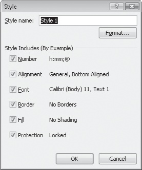
Clicking a style from the Cell Styles gallery applies the style to the selected cells, but Excel 2007 goes a step beyond previous versions of the program by displaying a live preview of a format when you hover your mouse pointer on it. If none of the existing styles is what you want, you can create your own style by displaying the Cell Styles gallery and, at the bottom of the gallery, clicking New Cell Style to display the Style dialog box. In the Style dialog box, type the name of your new style in the Style Name field, and then click Format. The Format Cells dialog box opens.

After you set the characteristics of your new style, click OK to make your style available in the Cell Styles gallery. If you ever want to delete a style, display the Cell Styles gallery, right-click the style, and then click Delete.
The Style dialog box is quite versatile, but it's overkill if all you want to do is apply formatting changes you made to a cell to the contents of another cell. To do so, use the Format Painter button, found in the Home tab's Clipboard group. Just click the cell that has the format you want to copy, click the Format Painter button, and select the target cells to have Excel 2007 apply the copied format to the target range.
In this exercise, you will create a style, apply the new style to a data label, and then use the Format Painter to apply the style to the contents of another cell.
Note
USE the HourlyExceptions workbook. This practice file is located in the DocumentsMicrosoft Press2007OfficeSBS_HomeStudentExcelAppearance folder.
OPEN the HourlyExceptions workbook.
 On the Home tab, in the Styles group, click Cell Styles, and then New Cell Style.
The Style dialog box opens.
In the Style name field, type Crosstab Column Heading.
Click the Format button.
Click the Alignment tab.
In the Horizontal list, click Center.
Center appears in the Horizontal field.
Click the Font tab.
In the Font style list, click Italic.
The text in the Preview pane appears in italicized text.
Click the Number tab.
In the Category list, click Time.
In the Type pane, click 1:30 PM.
Click OK to accept the default time format.
The Format Cells dialog box closes, and your new style's definition appears in the Style dialog box.
Click OK.
The Style dialog box closes.
Select cells C4:N4.
On the Home tab, in the Styles group, click Cell Styles.
Your new style appears at the top of the gallery, in the Custom group.
Click the Crosstab Column Heading style.
Excel 2007 applies your new style to the selected cells.