
Overview of Disks
Disk technology has advanced tremendously in the past few years. Providing virtually unlimited on-line storage at extremely low cost, it enables highly complex software to be created without worry about size limitation, as well as frees users from having to be conscientious about what and how much data to retain. While disk storage may not be the central engine of a computer, its dynamic growth and development certainly played a pivotal role in fostering the tremendous advancement of computer systems from their early days to where they are today. Imagine what the personal computer would be like if its secondary storage had a capacity of only tens of megabytes instead of the tens of gigabytes that we now take for granted.
From its original inception as a double-freezer-size storage device for accounting application, the impact of disk-based storage has now gone beyond computer systems. It is moving into our everyday lives as pervasive embedded devices in consumer products such as digital video recorders, cameras, music players, automotive navigation systems, cell phones, etc. While the basic principles of disk drives remain the same, such applications call for a different set of requirements and performance characteristics.
Despite today’s disk drives becoming commodity products, the fact remains that a disk drive is a highly complex electro-mechanical system encompassing decades of finely honed research on a vast multitude of diverse disciplines. They run the gamut of physics, chemistry, material science, tribology, electrical and electronics engineering, mechanical engineering, coding theory, computer science, and manufacturing science. Part III of this book presents a high-level discussion of disk drive technologies involving these topics, just sufficient for the reader to understand how a disk drive works. This provides the background knowledge to study some of the design issues and trade-offs that can affect the performance of a disk drive and disk-based storage subsystems. Emphasis on performance discussion is the major attribute that distinguishes this book from other previous books on disk drives.
While the disk section of this book is focused on the physical disk drive itself, there are two supporting software constituents that reside in the host system, namely the file system and the disk driver. Unlike the DRAM main memory which a user’s program makes direct access to, an operating system typically provides the service for storing and retrieving data to and from a disk-based storage on behalf of the application program. The file system and the disk driver are the two operating system components providing this service. The reader is assumed to have some general knowledge about file systems and disk drivers.
16.1 History of Disk Drives
Before the invention of the magnetic disk drive, magnetic tapes, introduced by IBM in 1953, were the dominant mode for secondary storage. The performance disadvantages of tapes are obvious. To locate a piece of data, the tape must be sequentially searched, which can easily take many seconds and even minutes. A different kind of device having random-access capability would provide much better performance and therefore be more desirable. In 1950, Engineering Research Associates of Minneapolis built the first commercial magnetic drum storage unit for the U.S. Navy, the ERA 110. It could store 1 million bits of data. Magnetic drums, announced in 1953 by IBM but not shipped until December of 1954, allowed for fast random access of data, but were not able to achieve as high a recording density as tapes. The higher cost of magnetic drums limited their use to serving only as main memory for the IBM 650, the first commercial general-purpose computer from IBM.
In 1952, Reynold Johnson of IBM, a prolific inventor of electro-mechanical devices, was asked to start a new research team in San Jose, CA. One of his mandates was to create a better technology for fast access to large volumes of data. It was decided early on to use inductive magnetic recording as the base technology, as it was a proven technology with the magnetic tapes and drums. The open question was what configuration the new device should be for achieving fast random access at low cost. In the end, a new, flat platter design, as first reported in 1952 by Jacob Rabinow of the National Bureau of Standards, was chosen over a simpler cylinder concept. Johnson accurately foresaw its better potential for future improvements.
RAMAC (Random-Access Method of Accounting Control), as the first disk drive1 system was designated, was successfully demonstrated in 1955 [Stevens 1981, 1998]. The 1-ton, double-freezer-size disk drive (see Figure 16.1) consisted of fifty 24” diameter aluminum disks mounted on a common shaft. The shaft was driven by an AC motor spinning at 1200 rpm. The disks were coated on both sides with a magnetic iron oxide material, a variation of the paint primer used for the Golden Gate Bridge, so there were 100 recording surfaces. The whole disk stack was served by two read/write heads shuttling up and down the disk stack to access the selected platter (see Figure 16.2). Data is stored on 100 concentric recording tracks per surface. The original RAMAC had a total capacity of 5 million characters (7 bits each), achieved with an areal density of about 2000 bits per square inch. The linear bit density varied from 100 bits per inch at the innermost track to 55 bits per inch at the outermost track.2 The average access time for any record was around 1 s, a remarkable achievement at the time. The prototype was so successful that in 1956 it was marketed as RAMAC 305, the first commercial magnetic disk drive.


16.1.1 Evolution of Drives
Since the beginning, and continuing to today, four major forces drive the continual developments and evolutions in disk drive technologies, namely capacity, cost, performance, and reliability. Computer users are always hungry for more storage space. In the early days, only the biggest systems of Fortune 500 companies could afford to add a disk drive to their machines. Lowering the cost would help to expand the number and the variety of applications. While faster than tapes, disk drives were, are, and always will be orders of magnitude slower than the host system’s main memory. There is always the pressure for drives to narrow this gap, especially with the ever-improving main memory speed a moving target. Finally, with more and more critical information being placed on-line, the reliability of disk drives where such data is stored becomes more and more critical. Data integrity and data availability are both not only desirable, but absolutely essential in many cases.
Over the past half century, disk drives have undergone many improvements over the original RAMAC [Harker et al. 1981]; yet the underlying principles of operation remain essentially the same. While evolutions in the disk drive came in many forms and occurred in different components, they all have a common theme: miniaturization. It is the key to increasing the recording density, lowering cost, and improving performance. Oftentimes, miniaturization was achieved by coming up with more integrated, and sometimes simpler, designs. As a result, reliability and manufacturing efficiency were also improved. The relentless pursuit of better performance and higher reliability created many intriguing problems and challenges and fostered the inventions of some interesting approaches.
One key invention in the realization of the disk drive was to “fly” the read/write head over the recording surface with a constant, but close spacing. In the original RAMAC, this was achieved with a hydrostatic (pressurized) air bearing, wherein compressed air was forced out of tiny holes on the head’s surface. One early and very important evolution was the introduction of the hydrodynamic (self-acting) air bearing utilizing a contoured structure called a slider to carry the head. This important simplification, introduced in 1962 in the IBM 1301, eliminated the need for compressed air. This made it feasible for each recording surface to have its own dedicated head, something that was not practical if compressed air was required. Any disk surface can now be selected by electronically activating its associated head. As a result, the average access time was drastically improved, to 165 ms in the IBM 1301. Most of the subsequent improvements in slider design were mainly in reducing its dimensions. The latest femto slider has a dimension of less than 1 mm × 1 mm.
In 1963, the concept of a removable disk pack was introduced. The IBM 1311 operated on swappable disk packs, each consisting of six 14-in. diameter disks. As the cost of a total disk subsystem was still very high at the time, this technique, borrowed from tapes, allowed the cost to be amortized over many times the capacity of a single disk stack. However, off-line storage would not have the access performance of on-line storage. Removable disk packs became the dominant form of disk drives for the next 13 years until fixed spindle drives returned in the IBM 3350. While fixed spindle remains the dominant disk drive configuration today, the removable disk pack concept continued to appear in various products, such as the once popular Iomega ZIP drive and, of course, the ubiquitous 5 1/4” floppy disks and 3 1/2” diskettes. Removable disk format is also the mainstay of all optical disk drives.
The concept of integrating the disks and the head arm assembly as a sealed unit was introduced by IBM in 1973 in the IBM 3340. Nicknamed the Winchester drive (it had two spindles with 30 MB each, thus “30/30 Winchester”), its concept of an integrated heads and disks assembly can be considered to be the predecessor of all of today’s hard drives (see head disk assembly, HDA discussion in Chapter 17, Section 17.2.9).
Up until the 1970s, disk drives remained big and expensive and were used exclusively in the realm of large computer systems. In 1980, Seagate revolutionized the disk drive industry by introducing the ST506, a 5 1/4” form factor disk drive for the nascent personal computer market. Eventually, the PC disk drive market far exceeded the enterprise storage market in terms of volume shipment. Undoubtedly, the personal computer would not have reached its success today if it was not for the availability of rapidly increasing capacity on-line storage at an ever-decreasing price.
Perhaps the most noticeable feature in the evolution of disk drives is its external dimension, dictated by the size of the disk platter being used. The RAMAC’s 24” disk platters gave way to 14” disks in 1963 when the IBM 1311 was introduced. This became the de facto standard for the next 16 years, not to be changed until the first 8” diameter disk was introduced in 1979. Seagate introduced the 5 1/4” form factor in 1980. The first 3 1/2” form factor drive was introduced by Rodime in 1983. Prairie Tek shipped the first 2 1/2” disk drive in 1988. As people started to realize the feasibility of the disk drive being used as a mass storage device outside the confines of computing, different sub-2” form factors were explored for various mobile applications. The 1.8” form factor was first pioneered by Integral Peripherals and MiniStor around 1991. In 1993, HP introduced the 21-MB Kitty Hawk, a 1.3” disk drive, but that form factor failed to take off. In 1999, IBM introduced the 1-in. microdrive, with a capacity of 340 MB at the time of introduction. Reaching a capacity of 8 GB in 2006, today it is successfully being used in digital cameras and MP3 players. The evolution history of disk diameter is plotted in Figure 16.3.

Control of early disk drive operations was handled entirely by an external controller often residing in the host computer. IPI (Intelligent Peripheral Interface) and, later, SMD (Storage Module Device) were some of the early standard interfaces used in disk drives for mainframes and minicomputers in the 1970s. The interface used in the first 5.25” disk drive ST-506, introduced in 1980, became a de facto standard for microcomputers until it was supplanted by ESDI (Enhanced Small Device Interface) and then eventually replaced by SCSI (Small Computer Standard Interface).
As disk drives acquired more functionality and intelligence, control gradually migrated into the drive to be handled internally and autonomously. SCSI was introduced in 1983 and officially became an ANSI standard in 1986 as X3.131-1986. The IDE (Integrated Device Electronics)/ATA (Advanced Technology Architecture) interface,3 a simpler and lower cost alternative to SCSI, was first introduced in products around 1987, though it did not become an ANSI standard until 1994 as X3.221-1994. The first high-performance Fiber Channel (FC) interface disk drives were shipped in 1997. Both SCSI and ATA are parallel interfaces, while FC is serial. Parallel interface suffers the disadvantage of bulky cables and short cable length. As a result, serial ATA (SATA) and serial attached SCSI (SAS) have recently been developed and standardized and will completely replace their parallel counterparts within a few years. Details on interface are covered in Chapter 20.
Evolutions of many of the less visible technologies within a disk drive, such as the recording head, media, codes, etc., are equally important, but not covered here and will be discussed in Chapter 17.
16.1.2 Areal Density Growth Trend
One of the most important parameters for a disk drive is its areal density, which is the number of bits that can be recorded per square inch. For a given disk diameter, this parameter determines the amount of data that can be stored on each platter. This, in turn, dictates the total storage capacity of a disk drive given the number of platters it contains. Even though there are many other contributing factors, ultimately, this is the single most important parameter that governs the cost per megabyte of a disk drive. It is the incredible and consistent rapid growth rate of areal density over the past 30 years that has driven the storage cost of disk drives down to the level that makes it still the technology of choice for on-line data storage. Areal density has reached the point where it is economically feasible to miniaturize disk drives, pushing them to fast becoming ubiquitous in our daily lives as tiny embedded components in many mobile products. As will be explained in Chapter 19, areal density also has a profound influence on performance.
The original RAMAC 305 had a lowly areal density of only 2000 bits per square inch. In late 2005, with the introduction of perpendicular recording, areal density had grown to an astounding 200 Gbits per square inch. This represents a growth of 100 million folds. The evolutionary history of areal density growth is summarized in Figure 16.4.

FIGURE 16.4 Evolution of areal density. Actual products of IBM/Hitachi-GST. Courtesy of Ed Grochowski of Hitachi Global Storage Technologies. CGR = compound growth rate.
Some of the technology improvements that have enabled areal density growth are the following:
• Thinner magnetic coating; improved magnetic properties
• Fabrication for smaller heads/sliders
• Flying height; reduced spacing between head and magnetic material, resulting in higher linear recording density
• Accuracy of head positioning servo, enabling tracks to be closer
Areal density, being a two-dimensional entity, consists of two components. The recording density in the radial direction of a disk is measured in terms of numbers of recording tracks per inch, or tpi (recording tracks are discussed in Chapter 18, Section 18.2). The recording density along a track is measured in terms of bits per inch, or bpi. For a rotating storage device spinning at a constant angular speed, the highest bpi is at the innermost diameter, or ID, of the recording area (a more detailed discussion can be found in Chapter 18). The product of tpi and bpi at the ID defines the areal density of a disk drive. The evolution history of bpi and tpi growth is plotted in Figure 16.5.

FIGURE 16.5 Evolution of linear recording density bpi and track density tpi. Actual products of IBM/Hitachi Global Storage Technologies. From multiple sources. CGR = compound growth rate.
To increase the areal density by a factor of 2, it might seem reasonable that bpi and tpi each be increased by a factor of ![]() . However, even though bpi and tpi are both components of recording density, they are, in part, affected by different technologies and mechanisms. Since 1990, tpi has been growing at a faster rate than bpi. As can be observed in Figure 16.5, bpi has roughly been increasing at an annual compound growth rate of 30% in recent years. On the other hand, the compound growth rate of tpi has been roughly 40% during the same period. Chapter 19 will discuss the impact of tpi and bpi on drive performance.
. However, even though bpi and tpi are both components of recording density, they are, in part, affected by different technologies and mechanisms. Since 1990, tpi has been growing at a faster rate than bpi. As can be observed in Figure 16.5, bpi has roughly been increasing at an annual compound growth rate of 30% in recent years. On the other hand, the compound growth rate of tpi has been roughly 40% during the same period. Chapter 19 will discuss the impact of tpi and bpi on drive performance.
16.2 Principles of Hard Disk Drives
While the first airplane flown by the Wright brothers at Kitty Hawk in 1903 may look quite different from today’s Boeing 777, many of the fundamental principles for powered flight have not changed. Both have wings to provide lift, engines to propel the plane forward, a movable rudder to control the yaw, and elevators to control the pitch. A similar parallel can be drawn between the first RAMAC machine and today’s disk drives, such as the microdrive (Figure 16.6). The physical appearances and dimensions of the two storage devices may seem very different, but their working principles and main components are quite similar, as explained below.

16.2.1 Principles of Rotating Storage Devices
The hard disk drive is not the only type of rotating platter storage device. The very first such device of this type is, of course, the phonograph, which stored audio information in analog form. Different types of rotating storage devices use different recording media for storage. Mechanical storage devices, such as the phonograph and the still-experimental atomic force microscopy (AFM) technology, store data as indentations on a recording surface. Optical storage devices, including CDs and DVDs, use variations in reflectivity for recording data. Magnetic storage devices record data with the magnetic polarization of ferromagnetic material.
Regardless of the recording method and the recording media, all rotating storage devices share some common features and operate on the same principles. They all use a platter to hold the recording material on one or both surfaces. They all have “heads,” which are transducers for converting the signal extracted from the recorded media (magnetic field, reflected light, or mechanical motion) into electrical signals, or vice-versa. A read element in the head is used to detect and retrieve the recorded data. For the read-only type of storage devices, such as DVD-ROM, this is the only type of head needed. For recordable devices, such as magnetic disks and DVD-RW, the head also contains a write element to write (record) the data onto the recording material. The functioning of the head and its elements depends on the type of storage mechanism.
The location of a data bit on a storage disk can be specified with two parameters or, more precisely, two coordinates. The first parameter is the radial distance from the center of the disk. This parameter defines a circle. The second parameter is the angular position of the location from a fixed reference axis. This is as shown in Figure 16.7. To access a bit of data, the head must be at the location where it is recorded or to be recorded. This can be accomplished in one of two ways: either the head moves to the bit location, or the bit location can be brought to where the head is. In all rotating storage devices, a combination of both methods i s used. The head is mounted on some movable mechanism which can place the head at any desired radial position. Again, the structure of the movable mechanism depends on the type of storage, thus the mechanism for carrying the laser and mirror used in optical recording is completely different than the structure for holding the magnetic recording head. The radial positioning of the head is commonly referred to as “seek.” Once it is at the target radial position, it essentially becomes stationary, making only minute adjustments to stay on track.

Next, the disk is rotated to bring the desired bit location to where the head is located. Unlike the head, the disk is constantly rotating. This is for performance reasons. First, the disk is much heavier than the head, and so it takes much more time and power to move it to a new angular orientation from a standstill. Second, data is accessed in quantities much larger than just a single bit. By constantly rotating the disk, many data bits are continuously brought under the head. An electric motor spins the disk platter, some at a constant rotational speed and some at a variable speed depending on the head location so as to maintain a constant linear speed of the recorded material under the head. More about these two methods will be discussed in Chapter 18.
All rotating storage devices have electronics for controlling the rotation of the disks and electronics for controlling the servo mechanism of the head positioning. The servo affects the seek time, which is an important factor in performance, and it will be discussed in Chapters 17 and 18 for hard disk drives. There are circuitries for converting between users’ data and the actual recorded signal. Details of this will be covered in Chapter 17, Section 17.3.3, for magnetic recording. Finally, there are electronics to handle the interface between the storage device and the host to which the device is attached, which will be discussed in Chapter 20.
More than one platter can be mounted in the same motor spindle for increased capacity. This adds a third dimension to the storage device, as illustrated in Figure 16.8. Since moving a shared head in this z-dimension, as was done with the original RAMAC, is a very slow mechanical process, it is desirable to have a dedicated head for each recording surface, as Figure 16.8 illustrates. Selection of storage location in this dimension then becomes simply electronically activating the right head. However, some recording technology, such as optical recording, may not be possible to implement such configuration in a cost effective manner.

16.2.2 Magnetic Rotating Storage Device—Hard Disk Drive
Magnetic recording technology is used in magnetic tapes as well as both fixed and removable media disk drives. Whether analog or digital, it consists of some type of magnetic storage medium, read and write heads to detect and induce a magnetic field, and recording channel electronics. The digital form of magnetic recording technology additionally requires data encoding and clocking logic for conversion between digital data and analog waveforms. It also must have some mechanism for controlling the designed spacing between the heads and the storage medium.
The rotating magnetic storage device is the result of combining magnetic recording technology with rotating recording technology. The resulting components of a magnetic hard disk drive are discussed in greater detail in Chapter 17. Refer to Chapter 17, Figure 17.8, for a view of some of these components. Briefly, a disk drive consists of one or more platters of magnetic media spun by an electric motor. When a biaxially oriented, polyethylene terephthalate material is used as the substrate of the disk platter, the storage device is a flexible media disk. When an aluminum-magnesium alloy or glass is used as the substrate material, the storage device is a hard disk drive. The recording media for magnetic hard disks is discussed in Chapter 17, Section 17.2.1. A magnetic field sensing read head and a magnetic field inducing write head are used for accessing data on each recording surface. Magnetic recording heads are covered in Chapter 17, Section 17.2.3. The mechanical structure that holds the heads is called the arm, and the mechanism for positioning the heads is called the actuator. They are described in Chapter 17, Section 17.2.4.
16.3 Classifications of Disk Drives
In the early days of data storage, there was only one class of disk drives—large disk drives attached to big computers. That picture began to change with the introduction of ST506 for the personal computer. Today, there are several ways disk drives can be classified.
16.3.1 Form Factor
One way to classify disk drives would be according to the dimensions of its external enclosure, or form factor. For reason of interchangeability, today drives usually come in one of four main standard sizes, namely 3.5″, 2.5″, 1.8″, and 1″. This dimension refers to the width of the sealed disk drive unit. The depth of the unit is longer than its width and is more or less also standard. The height is shorter and may come in one of two or three standard sizes for a given form factor. Around the 1980s, the 5 1/4” form factor, as pioneered by the ST506, was dominant, but had essentially disappeared by mid-1990s. Form factor alone is not always a good way to classify drives because two different drives with very different technologies inside and with very different functionality, performance, and reliability can have the same external form factor.
16.3.2 Application
Another way to classify a disk drive would be according to the platform in which it is being used. In the information technology (IT) world, traditionally there are server class drives for use in higher end or enterprise systems, desktop class drives for use in personal computers and low-end workstations, and mobile class drives for use in laptop or notebook computers. Each class of drives has different characteristics and requirements because of the application environment it is being used in. Server drives need to have high reliability and performance. Desktop drives must have low cost due to the highly price-competitive personal computer market. Low power consumption is an obvious yet important criterion for mobile drives. Today, the boundaries for this way of classification are starting to blur. As tremendous progress has been made in the reliability of all disk drives, some higher end system builders are beginning to use desktop drives in certain applications to take advantage of their low cost.
Almost coincidental with the start of the new millennium, disk drives have begun to move outside of the IT world and into consumer electronics (CE) applications. Such applications include digital video recorders, MP3 music players, game boxes, still and video digital cameras, cell phones, PDAs, and automotive applications such as GPS guidance systems. The list will continue to expand as the price of disk storage continues to fall. So far, most of these diverse applications have rather similar performance characteristics, and low cost is an important attribute for the disk drives being used. While highest possible capacity is always desirable, the size and power limitations of these consumer devices naturally dictate the form factor of the drives to be used. Thus, 1” microdrives are used in cameras and music players. On the other hand, home video recorders, which do not have any size or power limitation, are built with 3.5” disk drives to provide the most hours of recording.
16.3.3 Interface
Yet another way to classify disk drives is by the type of interface the drive provides. Current choices of interface are Fiber Channel (FC), parallel SCSI (Small Computer System Interface), parallel ATA (Advanced Technology Attachment), and the emerging serial ATA (SATA) and serial attached SCSI (SAS). A more detailed discussion of interface can be found in Chapter 20. Server class drives are available in either FC or SCSI interface. Desktop, mobile, and CE drives invariably come with an ATA interface, either the original parallel version or the newer serial flavor. Server class drives are more than twice as expensive as desktop drives. This association with interface leads some people to mistakenly think that SCSI drives are expensive because of the SCSI interface, when it is mostly the more costly technologies that go into a server class drive for achieving higher reliability and performance that makes it more expensive. As mentioned before, some storage systems are starting to use ATA desktop drives in certain applications to achieve a lower system cost.
The above various ways of classifying disk drives are summarized in Table 16.1. This is only a snapshot of 2007. A few years from now, the composition of this table may look different. Note that both SCSI and ATA can be either parallel or serial.

16.4 Disk Performance Overview
This section is a brief introduction to disk performance. It will define a few terms and set the background for the in-depth performance discussions that are to follow in some of the coming chapters. In particular, Chapter 19 discusses how a drive’s physical design parameters can affect the user performance. Chapter 21 presents various methods of operation within a disk drive to improve its performance. Testing of drive performance is discussed in Chapter 23.
16.4.1 Disk Performance Metrics
There is no single standard for defining disk performance. Depending on the requirements of the application or user, disk performance can be evaluated in a variety of ways. The most commonly used metrics of drive performance are discussed here.
Response Time and Service Time
A common measure of disk performance is the response time. This measures the elapsed time from when a command4 is issued to the disk drive to when data transfer is completed and the disk drive signals completion of the command. When a command is issued to the disk drive one at a time (this is called synchronous I/O), response time is the same as the drive’s service time. Response time is basically a measure of how fast a drive is in servicing a request. Hence, it is a measurement of speed. Chapter 19 discusses many of the factors influencing response time.
The response time of one single particular I/O is usually not very interesting. The result of a sample of one is also often misleading. Thus, it is more common to quantify a drive’s performance by the average response time for a large number of requests. Sometimes, much information about the performance of a drive is lost by quantifying it with just a single number. A more illuminating method is to report the distribution of response times, i.e., by the use of a histogram. Finally, for better understanding of the performance behavior of a disk drive, it may be desirable to report response time by I/O type, such as reads and writes, random and sequential, etc. This is discussed further in Chapter 23, Section 23.2.
Throughput
Another measurement of drive performance is the throughput, or its capacity to handle work. Throughput is commonly measured in one of two ways: (i) the number of I/Os per second (IOPS) or (ii) the amount of data transferred per second, or transfer rate, often stated in megabytes per second (MB/s). Some people refer to transfer rate as bandwidth. These two throughput measurements are related by how much data is transferred for each I/O request (block size),
IOPS × average block size = transfer rate (EQ 16.1)
and, hence, are equ0ivalent ways of describing performance.
Throughput, by its very nature, is measured by the aggregate of many I/Os. Thus, “average” is implied here. As with response time, it may also be desirable to report throughput according to I/O type. IOPS is commonly used for reporting random I/O performance, while transfer rate is used for reporting sequential I/O performance.
Response Time vs. Throughput
When multiple commands are allowed to be queued up inside a disk drive, as shown in Figure 16.9, then the response time will also include the time that a command sits in the queue waiting for its turn to be serviced plus its actual service time. Response time and throughput are somewhat related and are generally inversely proportional to each other. Also, a drive with fast service time will yield high throughput. Their relationship is governed by queueing theory [Kleinrock 1975, Breuer and Baum 2006]. In general, it looks something like the graph in Figure 16.10. Throughput (IOPS), as seen by the user, is the rate at which the user’s requests arrive at the disk drive. A server’s utilization is defined as
utilization = arrival rate × service time (EQ 16.2)5

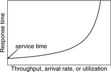
Assuming that the disk drive has a constant average service time, then utilization is directly proportional to arrival rate. Therefore, Figure 16.10 has the same general shape whether throughput, arrival rate, or utilization is plotted on the x-axis; only the scale will be different. The precise shape of the curve is determined by what the distributions of the I/O arrival time and the service time are. For example, when both times are exponentially distributed,6 the curve is given by
response time = service time / (1 – utilization) (EQ 16.3)
The service time is, of course, determined by the performance characteristics of the disk drive.
For detailed discussions on queueing, refer to Kleinrock [1975] and Brewer and Baum [2006]. Section 4 of Chapter 6 in the computer architecture book of Hennesy and Patterson [1996] also has a nice introductory discussion of this subject.
16.4.2 Workload Factors Affecting Performance
For a given disk drive, the response time and throughput that it can produce and be measured are dependent on the workload that it is given. The characteristics of a workload that can influence performance are the following:
• Block size: The sizes of the I/O requests clearly affect the response time and the throughput, since, when everything else is equal, a large block size takes longer to transfer than a small block size.
• Access pattern: Sequential, random, and other in between types of accesses will be discussed in greater detail in Chapters 21 and 23.
• Footprint: How much of the total available space in a disk drive is accessed affects the performance. A small fraction of the disk being accessed means the seek distances between I/Os would be small, while a large fraction of the disk being accessed means longer seeks.
• Command type: Read performance can be different from write performance, especially if write caching is enabled in the disk drive. Reads afford the opportunity for read hits in the drive’s cache which give much faster response time. Writing to the disk media may also take longer than reading from the media.
• Command queue depth: If both the disk drive and the host that it is attached to support queueing of multiple commands in the drive, throughput is affected by how deep a queue depth is being used. The deeper the queue is, the more choices are available for optimization and hence the higher the throughput. Command queueing will be discussed in Chapter 21.
• Command arrival rate: If command queueing is supported by the drive, response time is affected by the rate at which I/Os are being issued to the drive. If commands are issued at a higher rate, then more commands will be queued up in the drive, and a newly arrived command will, on average, have to wait longer before it gets serviced. Hence, response time will be higher. This is discussed previously in Section 16.4.1.
16.4.3 Video Application Performance
Video recording is a relatively new application for disk drives, and it has a different performance requirement than computer applications. Video needs to have the data ready to display every frame of a picture without miss. As long as data is guaranteed to be ready, there is no advantage to having the data ready quickly way ahead of time. Thus, the metric of performance for video application is how many streams of video that a disk drive can support and still guarantee on-time data delivery for all the streams. A home entertainment center in the near future will be required to record multiple programs and, at the same time, send different video streams to different rooms with support for fast-forward, pause, and other VCR-like functions. This type of throughput quantification has less to do with the speed of the disk drive rather than by how data is laid out on a drive, how the drive manages its buffer, and how a drive does its scheduling.
16.5 Future Directions in Disks
The demise of the disk drive as the most cost-effective way of providing cheap secondary storage at an acceptable level of performance has every now and then been predicted by some over the years. Such predictions have always turned out to be premature or “grossly exaggerated” as Mark Twain would put it. Magnetic hard disk drives will continue to be the dominant form of secondary storage for the foreseeable future. The transition of magnetic recording from that where magnetization is in the plane of the disk (horizontal magnetic recording) to one where magnetization is normal to the plane of the disk (perpendicular magnetic recording) is starting to take place and will help sustain the current pace of areal density growth. This continual growth in recording density will help to maintain the trend toward smaller and smaller form factors for disk drives.
As the cost of disk storage continues to drop, its application will expand beyond on-line data storage to near-line and even off-line data storage. These are applications traditionally served by tapes. To handle the large number of disk drives required for such applications in an enterprise system, the architecture of massive array of idle disks (MAID) has been created. In this architecture, at any point in time only a small fraction of the disks in the storage system are powered up and active to receive data, with the remaining vast majority of drives powered down. The drives being powered up are rotated among all the drives to even out their usage. This will significantly reduce the amount of power being consumed and, at the same time, extend the life of the disk drives.
Disk drives will also find more and more applications outside of the computing world. Already, disk drive-based personal video recorders (PVR) replacing VHS machines seem to be almost a foregone conclusion at this point. Other examples of applications in consumer electronics have already been mentioned earlier in Section 16.3. The penetration of disk drives into those markets can be expected to grow.
Just as disk drives today have become a commodity product, so too will small RAID (Redundant Array of Independent Disks) systems. In a few years it may become commonplace for us to have in our personal computer not a disk drive, but a storage “brick” inside of which are multiple disk drives, arrayed in some sort of RAID configuration. Such bricks will be the field replaceable units, rather than the individual drives themselves.
1Up until the 1990s, disk drive was also called DASD (pronounced “des-dee”) for direct-access-storage-device, a term coined by IBM.
2Recording density varied because each track held the same number of bits.
3It is nowadays commonly called simply ATA.
4A request or command to a drive is oftentimes referred to as an I/O (input/output) operation or request. In this book, the terms request, command, I/O, and I/O request are used interchangeably.
5Equivalent forms of this equation are utilization = service time/inter-arrival time and utilization = arrival rate/service rate.
6In queueing theory, such a single server queue is called an M/M/1 queue.