
The Physical Layer
This chapter presents a high-level overview of magnetic recording and the major physical components of a disk drive. Continual research and development have been widely conducted for the past 50 years in the many disciplines involved, driven by intense competition not only among disk drive makers, but also from other competing technologies eager to supplant disk drives as the low-cost storage technology of choice. The goal of this chapter is to provide enough general background knowledge of how a disk drive is created so as to facilitate the understanding of other chapters to follow.
The chapter is divided into three main sections. Section 17.1 is a brief review of the physics behind magnetic recording. Section 17.2 describes the electromechanical and magnetic components of a disk drive. The electronics integrated into today’s disk drives are discussed in Section 17.3.
17.1 Magnetic Recording
An essentially non-mathematical overview of magnetic recording principles is discussed here, introducing some of the more frequently used terms along the way [Bertram 1994, Mee & Daniel 1996]. The ingredients of magnetic recording are materials that can be permanently magnetized, magnetic fields, and the interaction between the two. Permanently magnetizable materials are called ferromagnetic materials, and they provide the storage media for recording due to the non-volatility of its magnetization. Externally applied magnetic fields are used to induce magnetism in ferromagnetic materials and, hence, are the means for recording when such fields can be controlled. Finally, by sensing the magnetic fields of magnetized ferrormagnetic material, what has been recorded can be detected and retrieved. That, in a nut shell, is how data is stored, written, and read in magnetic recording.
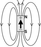
Permanent magnets occur in nature, and their existence, as well as their magnetic properties, was discovered many hundreds of years ago. A magnet always comes with two poles of opposite polarity. Hence, a magnet is one form of a magnetic dipole. A dipole is simply a pair of magnetic poles of opposite polarity. While these two polarities are commonly referred to as north (N) and south (S), in scientific literature they are oftentimes labelled as positive (+) and negative (–) poles instead. By convention, lines drawn in diagrams to represent magnetic fields are shown as flowing from the +ve (N) pole to the –ve (S) pole, as illustrated in Figure 17.1. A magnet can be simply represented by a thick arrow pointing from the – ve pole to the + ve pole; the + / – or N/S labelling is superfluous.
17.1.1 Ferromagnetism
Ferromagnetic materials are substances that can be permanently magnetized, which means that once they have been magnetized they stay magnetized, even after the mechanism or driving force for magnetizing them has been removed. Iron, nickel, cobalt, and some of the rare earth elements such as gadolinium and dysprosium are ferromagnetic materials. One can also make amorphous (non-crystalline) ferromagnetic metallic alloys by rapid quenching of certain liquid alloys.
The spin of an electron has a magnetic dipole moment and creates a magnetic field. In many materials the electrons come in pairs of opposite spin, cancelling one another’s dipole moments. However, atomswith unpaired electrons will have a net magnetic moment from spin. Ferromagnetic materials have such electrons, and they exhibit a long-range ordering phenomenon at the atomic level in which the unpaired electron spins line up parallel with each other in a region called a domain. This long-range order is remarkable in that the magnetic moments of neighboring atoms are locked into a rigid parallel order over a large number of atoms in spite of the thermal agitation which tends to randomize any atomic-level order. Within the domain, the magnetic field is strong. In a bulk sample, however, the material will usually be unmagnetized because the many domains will themselves be randomly oriented with respect to one another. This is illustrated in Figure 17.2(a).
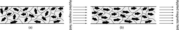
FIGURE 17.2 Domains of ferromagnetic materials: (a) before subject to external magnetic field and (b) with external magnetic field applied.
Ferromagnetism manifests itself in the fact that when a small external magnetic field is applied, the magnetic domains will line up with each other (as shown in Figure 17.2(b)), and the material is said to be magnetized. The driving magnetic field, now reinforced with the magnetic field generated by the magnetized material, will then be increased by a large factor which is expressed as the relative permeability of the material. Thus, a piece of ferromagnetic material initially has little or no net magnetic moment. However, if it is placed in a strong enough external magnetic field, the domains will reorient in parallel with that field. Furthermore, and importantly, the domains of ferromagnetic materials will retain much of this new parallel orientation when the field is turned off, thus creating a permanent magnet.
Although this state of aligned domains is not a minimal-energy configuration, it is extremely stable. However, all ferromagnets have a maximum temperature where the ferromagnetic property disappears. This temperature is called the Curie temperature. As temperature increases, thermal oscillation, or entropy, competes with the ferromagnetic tendency for spins to align. When the temperature rises beyond the material’s Curie temperature, the material can no longer maintain its state of magnetization without the aid of an external field.
17.1.2 Magnetic Fields
A magnetic field is a region of space where magnetic forces are present. Magnetic forces are produced by the movement of electrically charged particles. A wire carrying electrical current is really a stream of flowing electrons (moving in the opposite direction of the current, as defined by convention), and hence, it generates a magnetic field around it, as shown in Figure 17.3(a). The magnetic field created by one small current is weak. However, when the wire is wrapped around many times to form a coil, all the magnetic fields generated from each turn reinforce each other and result in a strong and nearly uniform magnetic field in the center of the coil. Such a coil is called a solenoid, as shown in Figure 17.3(b).
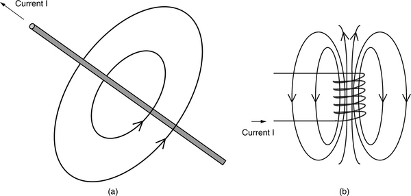
The magnetic field of a solenoid is similar to that of a permanent magnet (shown earlier in Figure 17.1). This is not a coincidence. An electron orbiting around the nucleus of an atom is a form of charged particle in motion and, hence, creates a magnetic field. Additionally, electrons that rotate about their own axis (spin) also create a magnetic field from that motion. When that atom does not have another electron spinning in an opposite direction to cancel that magnetic field, the atom will have a net magnetic field. When a large assembly of such atoms is lined up in the same direction, as in ferromagnetic materials, their individual magnetic fields reinforce each other, and a strong net magnetic field becomes detectable externally.
The strength of a magnetic field is a measure of its magnetic force at a given location of the field. By convention, it is represented by the symbol H. Unfortunately, H and the other magnetic measurements to be defined here can be given in several different units. In an MKS (meter-kilogram-second) system, H is given in amperes per meter (A/m). In a CGS (centimeter-gram-second) system, it is given in oersted (1 oe = ![]() ).
).
The magnetization of a magnetized material is defined as the density of its magnetic strength, called dipole moment, i.e., dipole moment per unit volume. By convention, it is represented using the symbol M. In an MKS system, M is also given in amperes per meter (A/m). In a CGS system, it is given in electromagnetic units (emu) per cubic centimeter (1 emu/cc = 103 A/m).
The lines of force surrounding a permanent magnet are called its magnetic flux, denoted by the symbol F. The amount of flux per unit area perpendicular to the magnetic flow is called the magnetic flux density, also known as magnetic induction. It is usually represented with B. In an MKS system, it is given in webers per square meter (W/m2), while in a CGS system, its unit is gauss (1 G = 10–4 W/m2). In magnetism, B is oftentimes used in formulas instead of H. In free space, the relationship between H and B is given by
where l0 is called the permeability of free space, and it is assigned the value
17.1.3 Hysteresis Loop
The capability of ferromagnets to stay magnetized after being subjected to an external magnetic field, i.e., to remember their magnetic history, is the very basis of magnetic recording. The magnetization M of a ferromagnetic material as a function of the externally applied magnetic field H is described by a hysteresis loop plot. Figure 17.4 shows a typical hysteresis loop. It can be seen from Figure 17.4 that the magnetization is not a unique function of the applied field, but depends on the state of the ferromagnetic material when the field is applied. This state is governed by the magnitude and the direction of previous applied fields.
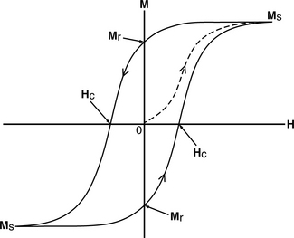
FIGURE 17.4 Hysteresis loop. The resulting amount of magnetization M when a magnetic field H is applied is dependent on the state of the ferromagnetic material.
Starting in the non-magnetized state of the ferromagnetic material, as the magnetic fields increases from 0 in the positive H direction, the magnetization of the material increases following the path of the dashed line, which is called the material’s magnetization curve. Eventually, a maximum value of magnetization is reached, where increasing H further will not result in any additional increase in M. This is called the saturation magnetization, Ms. When the applied field H is now reduced toward 0, the magnetization M is also reduced, but it no longer follows the magnetization curve; it follows the top curve of the hysteresis loop. At the point where no external magnetic field is applied, i.e., H = 0, the ferromagnetic material still exhibits a certain amount of magnetization. The value of this magnetization is called the remanent magnetization, Mr. A magnetic field must be applied in the negative H direction before the ferromagnetic material finally becomes demagnetized, i.e., M = 0. The value of H required to achieve demagnetization of the ferromagnet is called the coercivity, Hc. Thus, coercivity is a measure of how resistant the material is to demagnetization. Note that the hysteresis loop is completely symmetrical with respect to both the H and the M axes. Hence, the absolute values of Ms, Mr, and Hc are all independent of magnetic direction. The product Mr × Hc is a measure of the strength of the magnetic material.
Ferromagnetic materials can be broadly classified according to their magnetic behavior, which is manifested in their hysteresis loops. Figure 17.5(a) shows the hysteresis loop of a hard magnetic material. It is characterized by high coercivity and high remanence. Such materials are suitable for magnetic recording media. Figure 17.5(b) shows the hysteresis loop of a soft magnetic material. It is characterized by low coercivity and low remanence. Such materials are suitable for magnetic recording head applications.
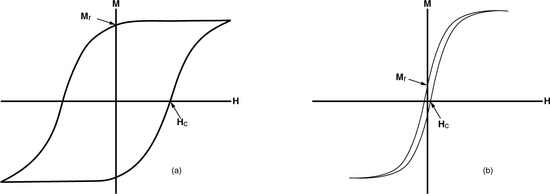
FIGURE 17.5 Hysteresis loops of magnetic materials: (a) hard magnetic material and (b) soft magnetic material.
Finally, a magnetic material has an easy axis, which is the direction that its magnetization prefers to point to. For the discussion in this chapter, we will assume magnetic recording materials that have easy axes parallel to the plane of recording. For such materials, longitudinal recording results, which is the type of magnetic recording used since the early days.
17.1.4 Writing
Writing is the process of recording a pattern of magnetization on the recording medium. Ideally, saturated recording, in which magnetic fields of sufficient strength to induce saturation magnetization are applied to the recording material, should be used in magnetic recording for the storage of digital data. This is as opposed to analog recording, such as cassette tape music and VHS video, where magnetic fields corresponding to recording signals of continuously varying magnitude and less than what is required for saturation magnetization are applied to the recording media. Since only the polarity, or direction, of magnetization needs to be distinguished in digital storage, magnetizing the recording medium to saturation will produce the strongest possible signal the material can provide, thus maximizing the signal-to-noise ratio.
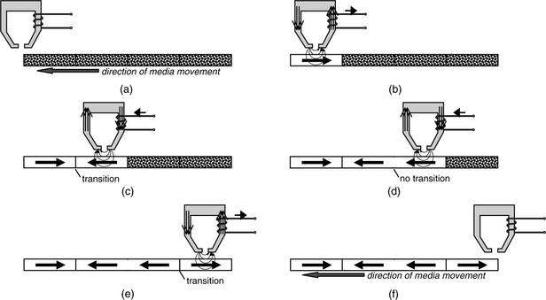
To illustrate the basic process of writing, consider a small, thin sample of magnetic medium and visualize that this sample consists of four recording compartments, as shown in Figure 17.6(a). Note that these compartments are only conceptual; they do not actually exist predefined in a real disk. A tiny external magnetic field is locally applied to the first compartment, which results in a left-to-right magnetization being induced in that compartment. This is as shown in Figure 17.6(b). Since ferromagnetic material is used, a remanent magnetization will remain in that compartment even after the external field is removed. Next, an external magnetic field is applied to the second compartment. This field is in the opposite direction of the previous field, and hence, a right-to-left magnetization is induced in the second compartment, as Figure 17.6(c) indicates. An external magnetic field, in the same direction as the previous field, is next applied to the third compartment, resulting in the third compartment being magnetized in the same polarity as the second compartment. Finally, a magnetic field in the opposite direction as that of the second and third compartments is applied to the fourth compartment, resulting in its left-to-right magnetization. When no more external fields are applied, the magnetic pattern of Figure 17.6(f) is left on the magnetic medium.
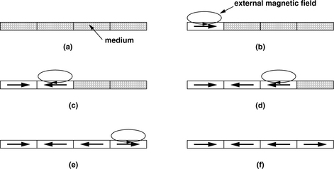
FIGURE 17.6 Write process example. (a) Medium before writing. Write magnetic field applied to (b) first compartment, (c) second compartment, (d) third compartment, and (e) fourth compartment, and (f) magnetic pattern in medium after writing.
We have just described the basic principle of writing the magnetic recording media. The mechanism with which electrical signals representing user’s data are converted to magnetic fields for writing is the function of the write head and the write channel electronics, which will be discussed later.
17.1.5 Reading
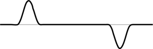
Reading is the process of determining the magnetic pattern that has been recorded in a medium. This is done by sensing the very weak magnetic field that emanates from the surface of each of the tiny magnetized compartments. Continuing with the above example, the magnetic fields just above the medium would look something like Figure 17.7.

Thus far, we have not defined how the magnetized compartments or their externally observable magnetic field can be used to represent binary data. Intuitively, one would think that the polarity of the recorded magnetization can be used directly to represent a 0 or a 1. For instance, we might define left-to-right magnetization to represent 0 and right-to-left magnetization to represent 1. Then, in the above example 0110 would have been recorded in the four compartments of the medium. However, finding a transducer that can detect the magnetic orientation of such very weak fields reliably posed a challenge during the formative years of magnetic recording. Instead, a different technique was used in the very early days of magnetic recording which is still universally used today. This technique operates on the change in orientation of magnetization rather than the orientation itself. This change in orientation is referred to as a transition. In our example, there is a reversal of magnetic orientation at the boundary between the first compartment and the second compartment, and another reversal is between the third compartment and the fourth compartment. There is no reversal of magnetic orientation at the boundary between the second and third compartments. By convention, a magnetic field reversal represents a 1, and the absence of a field reversal is used to present a 0. Note that which way a field is reversed is immaterial. In our example, therefore, the recorded magnetic pattern represents the binary sequence 101. Due to this method of data representation, writing needs to be done one complete block (called a sector) at a time; it is not possible to only write singly an individual bit. By sensing the presence or absence of field orientation reversals, or transitions, recorded data is read.
The read head is the transducer that detects magnetic field reversals and outputs electrical signals that can be processed and interpreted. The mechanism of how it does the detection and conversion is dependent on what type of read head is used. Various kinds of read heads will be discussed later.
17.2 Mechanical and Magnetic Components
While a disk drive’s working components have not changed much over the years, its size and construction has evolved greatly [Harker et al. 1981]. The packaging of all these components into a disk drive has also undergone dramatic changes, thanks to continual miniaturization, from the double-freezer-size RAMAC to the washing machine-size disk drives of the 1970s and 1980s and, finally, to the palm-size disk drives of the 1990s and today. Today’s disk drives all have their working components sealed inside an aluminum case, with an electronics card attached to one side. The components must be sealed because, with the very low flying height of the head over the disk surface, just a tiny amount of contaminant can spell disaster for the drive.
This section very briefly describes the various mechanical and magnetic components of a hard disk drive [Sierra 1990, Wang & Taratorin 1999, Ashar 1997, Mee & Daniel 1996, Mamun et al. 2006, Schwaderer & Wilson 1996]. The desirable characteristics of each of these components are discussed. The major physical components are illustrated in Figure 17.8, which shows an exposed view of a disk drive with the cover removed. The principles of operation for most components can be fully explained within this chapter. For the servo system, additional information will be required, and it will be described in Chapter 18.
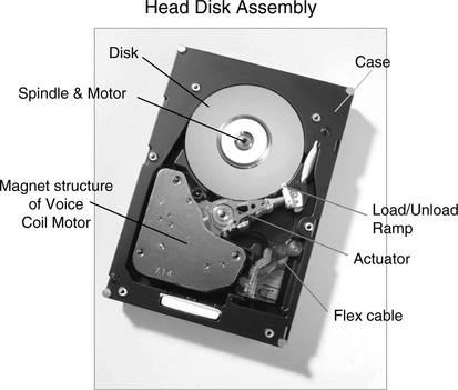
FIGURE 17.8 Major components of today’s typical disk drive. The cover of a Hitachi Global Storage Technologies UltraStar™ 15K147 is removed to show the inside of a head-disk assembly. The actuator is parked in the load/unload ramp.
17.2.1 Disks
The recording medium for hard disk drives is basically a very thin layer of magnetically hard material on a rigid circular substrate [Mee & Daniel 1996]. A flexible substrate is used for a flexible, or floppy, disk. Some of the desirable characteristics of recording media are the following:
• Thin substrate so that it takes up less space
• Light substrate so that it requires less power to spin
• High rigidity for low mechanical resonance and distortion under high rotational speed; needed for servo to accurately follow very narrow tracks
• Flat and smooth surface to allow the head to fly very low without ever making contact with the disk surface
• High coercivity (Hc) so that the magnetic recording is stable, even as areal density is increased
• High remanence (Mr) for good signal-to-noise ratio
• A square hysteresis loop for sharp transitions (to be discussed in Section 17.2.3)
Magnetic material is composed of grains of magnetic domains, as previously illustrated in Figure 17.2. The grain size of a material strongly affects its magnetic properties and the media transition noise. More grains at a transition boundary produce less noise and are therefore desirable. Yet, if grains size is decreased too much to accommodate higher tpi, the grains may become magnetically unstable.
Substrates
Up until the 1990s, aluminum was exclusively the material of choice for the hard disk substrate. More recently, electroless nickel-phosphorus plated aluminum has been used, which provides a surface capable of being polished to a high degree of smoothness. It is still the most common type of substrate in use today, mainly because of its low cost. However, there is a limit to how flat its surface can be polished, and the softness of aluminum makes it susceptible to accidental head slaps.
Glass and ceramics have been considered for many years as substrate materials, but only in recent years has glass been adopted in real products. The brittleness of glass has become less of a concern as disk diameter shrinks. Though costing more than aluminum, its ability to be polished to a very fine surface finish makes it an attractive alternative. Additionally, its hardness makes it less susceptible to head slap, and it is therefore a better choice for mobile applications. Its higher tensile strength also allows disks to be thinner.
Magnetic Layer
For the first 25 years of disk drives, what is known as particulate media was used exclusively in disk drives. With this type of magnetic coating, dispersions of magnetic particles in organic binders of polymer resins and solvents are essentially spray-painted onto a rotating substrate. Any excess “paint” is spun off by the rapid spinning of the disk, resulting in a thin film of polymer-magnetic particles. Before the film is dried, a magnetic field is applied to align the particles circumferentially to enhance their magnetic properties. Baking in an oven bonds the film onto the substrate. Finally, buffing and applying a coat of lubricant finish off the steps in creating a particulate media disk.
The most commonly used magnetic material in particulate media is particles of gamma ferric oxide, which are acicular in shape. Later developed particles include cobalt-modified gamma ferric oxide, chromium dioxide, metal particles, and barium ferrite. However, such newer particulate developments are applied more to flexible substrates, as thin film media made particulate media obsolete for hard disks.
With thin film media, a thin layer of magnetic metallic thin is deposited and bound directly onto the substrate without the use of polymer. The clear advantage of thin film media over particulate media is that more magnetic material is available as it is not being diluted by a non-magnetic binder. This enables a thinner layer of magnetic material to be used, which is a good thing because that allows narrower transitions to be written. Narrower transitions mean higher areal density.
Early methods of making thin film media include electroplating, chemically plating, and depositing onto the substrate by heating the desired material in a vacuum. The current method of production uses sputtering. Sputtering is performed by applying a high voltage across a low-pressure gas (argon is universally used), resulting in a plasma of electrons and argon ions in a high-energy state. The target magnetic material is bombarded by the energized argon ions accelerating toward it, displacing its surface atoms. The atoms are ejected with enough velocity to travel to the substrate and bond with it, resulting in the film of magnetic material on the substrate.
Disk Structure
A magnetic disk actually consists of more than just a substrate and a magnetic coating. Figure 17.9 shows a cross-section view of a typical thin film disk using an aluminum substrate. Starting from the bottom, above the substrate is a sublayer of nickel-phosphorus, which provides a much harder surface than aluminum, allowing it to be polished to a higher degree of smoothness and at the same time presenting a more damage-resistant surface. Next is an underlayer of chromium. Its purpose is to set up a desirable microstructure that the magnetic layer material is to replicate when deposited on this underlayer. The magnetic layer invariably uses some cobalt alloy, as cobalt alone does not have sufficient coercivity. Chromium is quite commonly used as one of the alloy metals. The thickness of this layer and grain size have a strong effect on coercivity and squareness. Grain size is influenced by rate of deposition, temperature of substrate, and other factors.
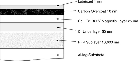
A layer of exposed magnetic material would leave it unprotected from potential scratches and corrosion. Therefore, a layer of wear-resistant overcoat is needed. The material for this layer should, naturally, be hard but not brittle, and it should be chemically inert but bond well to the magnetic layer. Today, the most common overcoat material is hard carbon, sputtered onto the disk. Finally, a very thin layer of lubricant is applied for reducing any wear and friction between the head and the disk.
17.2.2 Spindle Motor
For the disk media platter to rotate, it is rigidly attached to a spindle, and the spindle is driven by a motor [Shirle & Lieu 1996]. In the earliest days, synchronous AC motors were used, which phase locked to the 60 Hz of power lines to provide speeds such as 1200, 2400, and 3600 rpm. The spindles were belt driven by such AC motors, though direct drive was later introduced also. The resulting rotational speed was not very precise, but was acceptable for the relatively low bits per inch (bpi) in those times.
As the size of disk drives shrank, and the technology for low-cost switching control of DC motors became available, the AC disk drive motor became obsolete. Today, compact and efficient DC motors with the spindles directly integrated are universally used in all disk drives. Three-phase, eight-pole motors are typical. The motor with its stationary stator is attached to the base casing of the disk drive. The rotor is part of the outer sleeve of the motor which forms the spindle onto which the disk platters are mounted. Hence, the spindle is driven directly by the motor. Speed is electronically governed using servo control (see Section 17.3.4). Figure 17.10 is a photo of a cutaway spindle motor.

Ideally, the spindle drive motor should have the following characteristics:
• High reliability. If the motor does not spin properly, the disk drive is dead. Therefore, the motor must be able to run for many years and be able to go through tens of thousands or even hundreds of thousands of start/stop cycles.
• Low vibration. Vibration affects the ability of the head to stay in a stable position relative to the platter, thus impacting performance. This can also affect areal recording density.
• Minimal wobble. Wobble in the disk drive is known as Non-Repeatable Runout (NRRO). NRRO is a main contributor to track misregistration (TMR).1 Besides impacting performance, it is also an inhibitor to increasing tracks per inch (tpi), as it prevents tracks written to the disk from being perfectly circular.
• Low power consumption. Power causes heat, which must be dissipated or else it will shorten the life of the disk drive. For mobile applications, low power consumption is also important for making a battery last longer.
• Low acoustic noise. This is especially important for disk drives used in consumer electronics.
• High shock tolerance. This is true of every component in the disk drive, especially one used in mobile applications.
Bearings
Bearings are needed to both support and separate the spindle hub from the stator shaft so that the spindle can rotate smoothly and quietly. For many years, time-tested metal ball bearings confined to raceways inside the spindle were used in spindle drive motors. However, there is limit as to how perfectly round these tiny balls can be manufactured. The raceway in which these ball bearings run is not 100% perfect either. As mentioned, NRRO is a significant contributor to TMR. Spindle motors with ball bearings have an NRRO in the 0.1-microinch range. Additionally, materials in high-speed contact are subject to invariable wear and tear and are dependent on the age and durability of the lubricant protecting them. As the rpm of spindle drive motor increases over the years, heat and noise issues plus these limitations of ball bearing motors become more and more apparent. Figure 17.11(a) is a cross-section drawing of a ball bearing motor.

FIGURE 17.11 Cross-section drawing of spindle motors: (a) a ball bearing motor, and (b) a fluid dynamic bearing motor. (Drawing by Michael Xu of Hitachi GST.)
In recent years, disk drives have started to transition to spindle motors using fluid dynamic bearing (FDB). With FDB, the ball bearings are eliminated and replaced by a very thin layer of high-viscosity lubrication oil trapped in a carefully machined housing. Without the ball bearings and with the damping effect of a lubricant film, the FDB spindle motors run more quietly, showing roughly a 4-dBA decrease in acoustic noise. Furthermore, wobble is also greatly minimized, with NRRO in the 0.01-microinch range, which is an order of magnitude improvement over ball bearing spindle motors. Non-operational shock resistance is also improved due to increased area of surface-to-surface contact, while the lubricant film provides additional damping also. Initially, FDB motors will cost more. However, as production volume increases and manufacturing techniques mature, they will become cheaper to build than ball bearing motors as fewer parts are required. Figure 17.11(b) is a cross-section drawing of an FDB motor.
17.2.3 Heads
Heads are really the heart of a disk drive. In Section 17.1.4, the principle of recording information by applying an external magnetic field to magnetize and manipulate the orientation of magnetization of the magnetic media is qualitatively described. It is the write head that provides the source of the externally applied magnetic field. The detection of the magnetic recording, as described in Section 17.1.5 on the principle of retrieving magnetically recorded information, is performed by the read head.
Write Heads
The principle governing the operation of today’s write heads is exactly the same as that for the earliest recording heads [Robertson et al. 1997]. Nonetheless, the dimension, the geometry, the materials used, and the fabrication process have all evolved substantially over the years. While it is hard to tell by looking at the size and shape of today’s write heads and those of the RAMAC 350, all write heads are basically inductive ring heads.
The inductive write head basically consists of a ring core of magnetically soft material, such as ferrite, and a coil of wire wrapped around the core. There is a break in the core, forming a very short gap. The head “flies” very closely over the magnetic recording media, with the gap adjacent to the media. When an applied current passes through the coil, it induces a magnetic field inside the core, just like electromagnets, and hence the name inductive head. The direction of the magnetic field is dependent on the direction of the current in the coil. The two ends of the core at the gap form two magnetic poles of opposite polarities. At this gap, the magnetic flux leaks outside the core and fringes away from the gap. The leaked magnetic flux passes through the media, magnetizing the magnetically hard material of the media in accordance to its hysteresis loop characteristics and the amount of magnetic flux applied. This is illustrated in Figure 17.12. The space within which the magnetic field of the write head is strong enough for magnetic record to occur is sometimes called the write bubble. The magnetically hard media retains most of the magnetization after the magnetic field of the head is removed. This basic write head structure is used for both analog and digital recording.

In digital magnetic recording, the head/media/channel are designed such that when current is applied to the head, the resulting magnetic flux going through the media is of sufficient strength as to align the magnetic domains immediately adjacent to the head completely in the same direction as the applied magnetic field, regardless of the previous orientation. This is saturation magnetization. Since the magnetic media is moving under the write head due to the rotation of the disk platter, saturated magnetization occurs along the path (called track in recording terminology) that passes directly underneath the head, as long as the current is applied to the coil. When the current is switched off and then a current in the opposite direction is applied, the magnetic flux in the core reverses direction, and saturated magnetization in the opposite orientation as the previous magnetization now occurs in the magnetic media. This creates a transition in the media where magnetization changes from one orientation to the opposite orientation. This is shown in Figure 17.13. The transition is, of course, not a sharp line as drawn, but has a finite length to it, as the dipoles within it gradually change from predominantly pointing in one direction to predominantly pointing in the opposite direction. Media with a more square hysteresis loop will create sharper transitions. This transition length determines how closely the transitions can be spaced, which, in turn, determines the linear recording density. The sequence of pictorials illustrating the write process in Figure 17.6 can now be depicted with a write head as the source of the recording magnetic field, as shown in Figure 17.14. The size of the recorded bits relative to the head and its gap is not properly drawn to scale; in reality, the bit size is much smaller and closer to the dimension of the head’s gap. Writing, i.e., the creation of transitions, actually takes place at the trailing (left-hand side in Figure 17.14) side of the write bubble, as that is where the medium sees the final orientation of the magnetization field applied to it.

The desirable characteristics of the write head are the following:
• A narrow write width as it determines the tpi. This means that not only the width of the poles needs to be narrow, but also the gap between the pole needs to be short, or else there will be too much undesirable side writing.
• Core material must have high enough saturation flux density in order to produce enough magnetization to write media with ever-increasing coercivities.
• The inductance of the electric circuitry needs to be low enough to handle signals that are several tens of megahertz frequencies.
• Core material must be mechanically strong so that the poles are not easily damaged by contacts with the disk.
The first heads for the RAMAC 350 used permalloy (an alloy of nickel and iron) as the core material, and the coils were hand wound and assembled by former watchmakers. Needless to say, they share little of the above list of desirable characteristics. The shape and dimension of write heads have greatly evolved since then. Ferrites, which are ceramic-like compounds of iron oxides and other metallic oxides, replaced permalloy as the core material during the mid-1960s. While having other desirable characteristics, ferrites suffer from having a much lower saturation flux density than permalloy. By the mid-1980s, they simply did not have enough magnetic flux to work on the high coercivity of thin film disks. The solution was to add (sputter on) a thin layer of metallic material, commonly sendust which is an alloy of iron, aluminum, and silicon, to the poles near the gap. Hence, this type of head was called a metal-in-gap (MIG) head. The result is a head that has the high saturation flux density of sendust and the other desirable characteristics of ferrites.
MIG heads were gainfully used from the late 1980s to the early 1990s. However, the way they were manufactured, which involved mechanically grinding and polishing the ferrite material and actual winding of the copper coil, placed a limit on how small the dimensions of the head could be reduced to. Miniaturization of the head was the key to increasing areal density. With research starting in the 1960s, by the early 1980s, a completely new technique for manufacturing the heads was perfected. This new fabrication method leveraged on the tools and thin film technology of semiconductor manufacturing. By using lithography to define the features of the head and thin film deposition to construct all its components, including the core, the gap, and the copper windings, a miniature head with well-controlled dimension could be easily manufactured. Thin film heads, as these heads came to be called, were introduced in the IBM enterprise class of disk drives in 1980 and eventually became economical for all disk drives by the mid-1990s.
While the fabrication process of thin film heads differs from that for the ferrite and MIG heads, not to mention their miniaturized dimensions, functionally, they are really just like ferrite heads. Structurally, they are essentially three-dimensional inductive heads collapsed front to back to become almost just two-dimensional. Even the core material has gone back to permalloy, the original material used in the RAMAC 350 heads. Figure 17.15 illustrates conceptually the typical construction of a thin film head, fabricated using semiconductor technology. While the front-to-back spacing is much more compressed, and the coil takes on a flattened arrangement, functionally, it is exactly an inductive head.

FIGURE 17.15 Conceptual drawing of a fabrication of a thin film inductive head. (a) Deposit permalloy film to form bottom yoke. (b) Add coil. (c) Add top yoke/pole and coil connector. Top yoke is connected to bottom yoke under the oval at the top. (d) Side view. (Artwork by Michael Xu of Hitachi GST.)
Read Heads
For reading in digital magnetic recording, the read head detects the transitions that are recorded in the media. Transitions detected in the sync field (to be described in more detail in Chapter 18, Section 18.1.3) are used to establish the clock (self-clocking) for data reading. In the data field, each transition is used to represent a binary “1,” while the absence of a transition in a clocked period represents a binary “0,” as discussed earlier in this chapter. The read channel samples at each clock interval the signal coming out of the read head to check for the presence or absence of transition.
Up until the introduction of the magnetoresistive head in 1991, the inductive head was used also for reading, in addition to its function as the write head. It operates on the well-known magnetic phenomenon that a change in magnetic flux inside a coil of wire would induce a voltage in that coil. In fact, Faraday’s Law provides that the induced voltage is
where N is the number of turns in the coil. While used as a read head, no current is applied to the coil by the drive’s electronics. As the media moves next to the head, its core collects the magnetic flux emanating from the recorded magnetization on the media. When it comes across a transition, a magnetic flux change occurs as the magnetic field reverses polarity, and this flux change induces a voltage in the coil which can then be detected by the read channel circuitry. Figure 17.16 shows the read voltage signal for the sample sequence of “101” of Figure 17.14. Equation 17.3 suggests that having more turns in the coil would increase the read signal; however, making N too large would increase the inductance of the head, limiting its high frequency, and hence high data rate, handling. Also, because the inductive head operates by detecting the rate of flux change, the higher the velocity is, the stronger the read signal. Thus, higher rpm and larger disk diameter are both favorable for inductive read heads.
While inductive read heads operate by detecting flux change, magnetoresistive (MR) heads operate by sensing the flux directly [Tsang et al. 1997, 1994]. There is a class of materials, of which permalloy happens to be one, which exhibits the phenomenon of magnetoresistance. Basically, when a magnetic field H is applied to such a material, its electrical resistance changes as a function of the angle θ between the resultant magnetization M and the direction of flow of an applied electric current, as shown in Figure 17.17, in accordance to
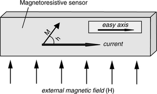
where ΔR is the change in resistance, R is the sensor’s nominal resistance, and CMR is the magnetoresistance coefficient of the material. For permalloy, CMR is about 2–3%.
By applying a constant current I to the MR sensor, the presence of a magnetic field is detected by a change in the voltage across this sensor in accordance with Ohm’s Law,
as a result of the change in the direction of magnetization due to the applied field H. Because a magnetic field is applied during fabrication of the sensor to give it an easy axis parallel to the current direction (θ = 0°), the biggest change in resistance will be when the external magnetic field H is in a vertical direction, either up or down, perpendicular to the current direction (θ = 90°), as shown in Figure 17.17. The biggest resistance change generates the biggest signal. Such vertical magnetic fields occur on the media’s recorded surface only at the transitions, where magnetic fields emanating from both sides of the transition are both either going up or going down, as can be seen in Figure 17.7. Common practice is to bias2 the MR sensor so that θ = 45° when no external magnetic field is present. As a result, the MR sensor generates up or down peak ΔV signals at transitions, with a waveform similar to the one shown in Figure 17.16 for inductive read heads. In order to prevent the MR sensor from detecting stray magnetic fields from adjacent transitions, the sensor is shielded front and back so that it can only “see” the magnetic field right underneath it.
The signal that can be created by an MR head is several times larger than that of an inductive read head. This is what drove the rapid increase in areal density after the introduction of the MR head in 1991. In fact, by increasing the sense current I, a bigger signal can be obtained, as Equation 17.5 indicates. However, heat and other heat-related issues limit the amount of current that can be practically applied. With no coil involved, the inductance of the MR head is so low that there is practically no limit to its high-frequency performance. Finally, since the MR head detects magnetic flux rather than the rate of change of flux, its signal is independent of the velocity of the media going by, unlike an inductive read head. This attribute is what makes small diameter drives with low rpm possible.
The MR sensor is constructed of a homogeneous ferromagnetic material such as permalloy. Around the early 1990s, researchers discovered that by constructing a composite sensor with multiple thin layers of different ferromagnetic and anti-ferromagnetic materials, made possible by the molecular beam epitaxy process, a sensor with giant magnetoresistance (GMR) results. An example of such a structure, as illustrated in Figure 17.18, consists of a “free” ferromagnetic layer and a “pinned” ferromagnetic layer separated by some non-magnetic material. The magnetization orientation of the pinned layer is fixed (pinned) by an adjacent layer3 of anti-ferromagnetic material (AFM). The GMR head was first introduced in a product in 1997.

Read/Write Heads
The transducers for reading and writing are oftentimes referred to collectively as the read/write head, or just simply the head. This is probably carried over from the earlier days when the inductive head was used for both reading and writing. Therefore, there is truly only one head. Requiring the same head to perform the read and the write functions means that compromise in design and performance would be necessary, as the optimum design for writing differs from that for reading.
Since the introduction of MR heads, the “head” is now really composed of an inductive write transducer and the MR (or GMR) read transducer. Having a separate read head and write head allows each design to be independently optimized for the function it needs to perform. The inductive head and the MR head are placed in tandem, with the write head going behind the read head, as illustrated in Figure 17.19. Standard practice today is for the write head to write a wider path (track) than the width of the read head, a technique called “write wide, read narrow,” by constructing the MR read sensor to be narrower than the width of the write pole tip, as shown in Figure 17.20. The advantage of such an approach is that the read head does not have to be perfectly centered over a track in order to have good read-back and not pick up noise from adjacent tracks. This also permits tracks to be placed closer together, thus increasing tpi.
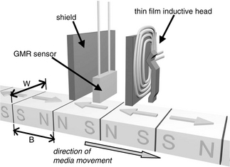
FIGURE 17.19 Conceptual drawing of a GMR read head with inductive write head. (Artwork by Michael Xu of Hitachi GST.)
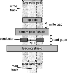
In Figure 17.19, the width of a track W is determined by the width of the tip of the trailing pole of the thin film head. The distance between the center of two adjacent tracks is called the track pitch. It is different from the width of a track because standard recording technique places a guard band between two tracks. The guard band provides protection against stray magnetic fields fringing from the sides of the write head which can partially erase adjacent tracks. It is this track pitch, rather than the track width W, that determines the tpi:
tpi = 1/track pitch = 1/(W + guard band width) (EQ 17.6)
but track pitch is pretty much dominated by track width. The distance B between two back-to-back transitions defines the flux change density, fcpi:
The actual linear bit density depends on the density ratio (DR) of data bits per flux change of the modulation code being used to encode the data bits (see Section 17.3.3):
bpi = DR × fcpi = DR/B (EQ 17.8)
However, many of the newer codes have a value quite close to 1 for DR, so it is not too far off to refer to B as the bit length. Historically, W has always been much larger than B. However, as areal density has increased over the years, tpi has been going up faster than bpi. As a result, the ratio of W to B has been dropping. Today, this ratio is close to 4:1.
The location of the outermost track that the write head can write is commonly referred to as the OD (outer diameter), while the innermost location is referred to as the ID (inner diameter).
17.2.4 Slider and Head-Gimbal Assembly
Contrary to what Figure 17.19 seems to portray, the heads don’t just magically float freely in space over the media. Rather, they are integrated as part of a mechanical structure whose function is to support the heads and to position them at the right location in order to access a specific bit of data.
The read/write transducers are bonded to a small piece of material called the slider. While the heads of the very earliest disk drives may actually slide on the media surface, hence the name, having the head in contact with the disk moving at high speed simply creates too much wear and tear for both the head and the media.4 For decades now the slider has been designed to ride hydrodynamically on a cushion of air, commonly called an air bearing, so as to maintain the proper spacing between the head and the media. This spacing is referred to as the flying height. There are many different designs for the air bearing surface (ABS): taper-flat, bi-rail, tri-rail, and tri-pad (Figure 17.21), just to name a few.

Maintaining the proper flying height is important, as it is one of the key factors that determines magnetic recording signals and linear bit density, as will be discussed in a later section. Yet, it is not a simple task as the linear velocity of the disk surface under the head, and hence the speed of air flow, varies with the radial position of the head. Flying height can also be affected by the skew angle of the head for rotary actuators (to be described later). Additionally, flying height must not be unduly affected by the atmospheric pressure of the environment that the disk drive operates in.
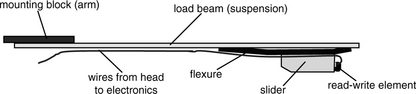
The slider is itself attached to the end of a load beam, also called a suspension or a disk arm (term probably comes from the similarity to the arm of a phonograph), by means of a flexure, as illustrated in Figure 17.22. Today’s suspension beam is typically triangular in shape with holes in the middle to reduce its weight. The flexure, acting as a gimbal, allows some limited rolling and pitching motion of the slider. The suspension is spring-loaded such that when the drive is not rotating it will press the slider against the disk surface to hold it in place, and when the disk is rotating at operating speed the head will be flying at the designed flying height. This structure of suspension, slider, and head is called the head-gimbal assembly (HGA).
As the size of the read/write element has been decreasing in size over the years, so has the slider. The generation of sliders introduced in 1980 was designated by the industry as the 100% mini slider (4.0 × 3.2 × 0.86 mm, 55 mg). In 1986 the 70% micro slider (2.8 × 2.24 × 0.6 mm, 16.2 mg) was introduced, followed in 1990 by the 50% nano slider (2.0 × 1.6 × 0.43 mm, 5.9 mg), and followed in 1997 by the 30% pico slider (1.25 × 1.0 × 0.3 mm, 1.6 mg). Finally, in 2003 the 20% femto slider (0.85 × 0.7 × 0.23 mm, 0.6 mg) was introduced. The percentage refers only to the length; the volume and mass actually shrink by a much higher percentage, e.g., the femto slider is only about 1% of the volume and mass of a mini slider. Also, the prefixes do not reflect their scientific meanings—they were more likely chosen just for marketing hype. There are several clear advantages of a smaller slider.
• A smaller slider means the suspension can also be made lighter. This combined reduction in mass reduces the power required for positioning of the heads and improves seek time.
• Reduction in mass also improves shock resistance and head-disk reliability.
• Smaller slider size makes it easier to respond to unevenness of a disk’s surface, hence reducing the variation in flying height.
• Because a slider cannot fly outside of the disk’s surface, having a smaller slider means more of a disk’s surface area is usable, and thus, storage capacity is increased. This is especially important for smaller diameter disks since a larger percentage of the disk becomes available.
• Smaller size means more sliders can be produced from a same size wafer, and thus, production cost is reduced.
17.2.5 Head-Stack Assembly and Actuator
All the head-gimbal assemblies of a drive, one per recording surface, are stacked together, lining up vertically, by attaching to a structure called the E-block. The wires from each head element are connected to a flex cable which also contains a tiny electronic circuitry called the arm electronics module (AEM). This complete structure of E-block, HGAs, and flex cable is called a head-stack assembly (HSA). The HSA is installed in a disk drive during final assembly as a single unit. To assemble a disk drive, the HSA is integrated with a voice coil motor (VCM) to form the actuator. These components are illustrated in Figure 17.23. The function of the actuator is to move the set of arms of the HSA so as to transport the heads from one radial position to a new target radial position in order to access the desired data. Because the arms are rigidly ganged together as a unit, all the heads move in unison. This movement of the heads is referred to as a seek operation.
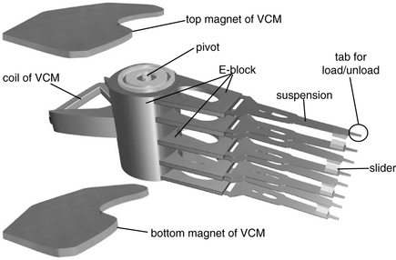
FIGURE 17.23 Illustrative example of an HSA and the components of a VCM for a rotary actuator. The flex cable and AEM are not shown. Drawing by Michael Xu of Hitachi GST.
The earliest disk drives made use of actuators that were driven with hydraulics! Mechanical detents were utilized to establish the cylinder positions, achieving a track density of less than 100 tpi. That was more or less the upper limit of what an open-loop control system could achieve. Mechanical tolerance of mechanical parts, variations in operating temperature together with materials having different coefficients of expansion, and vibrations all conspire to place such an upper limit. In order to further increase track density, an electronic servo system using closed-loop control logic was necessary. The IBM 3330, introduced in 1971, was the first drive to incorporate such a servo system. Since a special servo data pattern needs to be placed on the disk surface as part of the servo system, a more detailed discussion will be deferred to Chapter 18, which deals with all aspects of placing data on a disk surface.
The earlier actuators had the arms perpendicular to the tracks and moved them straight in and out across the surfaces of the disks, as shown in Figure 17.24(a). The first such linear actuator motors were made from loudspeakers with the cones removed, hence the name VCM. By passing current through the voice coil in one direction, the magnetic force due to the magnetic field of the rigidly mounted permanent magnet propels the HSA forward, and the heads would be seeking toward the ID of the disks. The amount of current applied determines the size of the electro-magnetic force generated, which, in turn, determines the motion of the HSA. By passing current in the opposite direction, the HSA is retracted, and the heads would be seeking toward the OD. Hence, by controlling the direction and the amount of current to the coil, the positioning of the actuator can be controlled.

FIGURE 17.24 Top views of actuators. (a) Linear actuator. (b) Rotary actuator, with the top magnets removed to expose the voice coil.
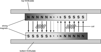
As disk diameter decreased, disk drive designs switched to a rotary type of actuator. In a rotary actuator the arms are held roughly tangential to the tracks, and the HSA swivels at a fixed pivot point in the actuator assembly, as shown in Figure 17.24(b). A coil is wrapped around a protruding metal piece at the back side of the E-block. Two strong magnets, each vertically magnetized with opposite polarities on each half, are placed above and below this coil such that the top magnet faces opposing polarities in the bottom magnet. Figure 17.25 shows a cross-section view of this arrangement.5 When current flows in the coil in one direction, electromagnetic force moves the coil to the right (in reference to the top view shown in Figure 17.24(b)), causing the actuator to rotate in a counter-clockwise direction. This results in the heads seeking towards the ID of the disks. When a current is applied to the coil in the opposite direction, the HSA rotates in a clockwise direction resulting in the heads seeking towards the OD. Once again, as with the linear actuator, by controlling the direction and amplitude of the current applied to the coil, the positioning of the rotary actuator can be controlled.
Today, the rotary actuator is used in all disk drives. Its advantages over a linear actuator are the following:
• Simpler design, and, hence, lower cost
• Smaller and lighter, which means faster seek performance and lower power consumption
The disadvantage of a rotary actuator is that there is only one radial position on the disk surface at which the head is exactly tangential to the track. Move away from that point and there is a small skew angle of the head with respect to the track underneath it. This would not be much of a problem if read and write used the same transducer. However, with MR/GMR heads, the read element is separate from the write element, as described previously. This means that when there is a skew angle, the two elements cannot be both dead center over the track at the same time. Hence, to switch between reads and writes, the servo actuator must do a slight position adjustment, called a micro-jog. Since the amount of micro-jog is dependent on the radial position and varies from head to head, the disk drive needs to go through a self-calibration during manufacturing to establish a micro-jog table for each of its heads.
It is by controlling the current in the coil of the (linear or rotary) actuator that its position is governed. However, if power to the drive is lost during a seek operation, no current can be applied to slow down and stop the actuator which is already in motion. To prevent a crash from happening, crashstops are installed at both ends of the actuator’s intended range of movement. This is not unlike the crashstops found at train station terminals.
Servo control of the actuator and seek performance will be covered in Chapter 18 and Chapter 20.
17.2.6 Multiple Platters
For a long time, when recording density was relatively low and the cost of a hard disk drive was relatively expensive, economics called for designing disk drives to hold as much data as possible. One way to do that is to use disks of large diameters. The disadvantages of larger diameter disks are the following:
• The seek stroke is longer, resulting in higher average seek time.
• The arms are longer, which, in turn, requires it to be thicker to provide the necessary stiffness. The result is an actuator with more mass, which means either the actuator will move slower (longer seek times) or more power will be needed to achieve the same performance as for a smaller diameter disk.
• A larger surface area means there is more air friction (windage). This translates to a greater power requirement to spin the disk at a given rotational speed.
• To attain the necessary stiffness so the disk does not sag, the thickness of the disk platter must increase proportionally to the increase in diameter. The total increase in weight from both a bigger diameter and more thickness means that even more power is needed to attain a given rotational speed.
For all of the above reasons, increasing the disk diameter in order to increase its capacity is not a good approach. Instead, the alternative is to grow in the z-dimension, namely increasing the number of disk platters per drive. This is a better approach for the same reasons as why increasing the diameter is a less desirable approach:
• The seek stroke is not increased, and the added weight to an actuator for having additional HGAs is minimal. Thus, seek performance is not affected.
• While the added platters do increase the total weight that the spindle motor must spin, it is less than the increase from a larger diameter disk, as the smaller diameter platters are thinner while providing the same rigidity.
An obvious disadvantage of having more platters is that more heads are required, and the head is one of the most expensive components of a disk drive. In recent years, due to the exponential growth in areal density, it has been possible to satisfy the per-drive capacity requirement of disk drive applications with fewer and fewer platters.
17.2.7 Start/Stop
When a disk drive is powered off or stops rotating, as when it is placed in an idle mode, something needs to be done to safeguard the heads from damage. There are two differing technologies for handling this, namely contact start/stop (CSS) and load/unload.
Contact Start/Stop
In this method, the head comes to rest on the disk surface as there is no longer an air bearing to support it [Bhushan et al. 1992]. When the disk starts spinning again, the head slides in contact over the disk surface until gradually an air bearing is formed under the slider and the head is lifted off the disk surface. With today’s high areal density, it is not a good idea to park the head on the portion of the disk where data is recorded, as the data with its tiny bit size can easily be damaged. Therefore, a designated landing zone is reserved on the disk surface for the head to park. While the landing zone can be placed outside either the OD or the ID, there are couple of reasons why placing it outside the OD is a bad design choice.
• The space reserved for a landing zone is lost for data storage. For a landing zone of a given width, the space lost is much bigger if it is at the outside of the disk.
• When the head slider is stopped in contact with the disk surface, there is an adhesive force, called stiction (short for static friction), that works against the disk spinning up, against which the drive must provide enough torque to overcome. A bigger torque is required if the stiction occurs at the OD than if it is at the ID. This means more power is used, and also perhaps a more powerful spindle motor would be needed to provide this larger torque.
For the above reasons, the landing zone is placed at the inside of the disk. To further reduce the effect of stiction, the landing zone is textured so that the total surface area in actual contact is reduced. During a normal shutdown, the disk drive controller firmware would instruct the actuator to position itself over the landing zone before spinning down the disk. To guarantee that in the event of an unexpected power loss the head still gets properly stowed away in the landing zone, some sort of auto-park feature is needed. Some older drives use a weak spring to pull the actuator to the landing zone. Newer drives use the kinetic energy of the spinning platters to generate back-EMF (electro-magnetic force) power from the spindle motor to move the actuator to the landing zone.
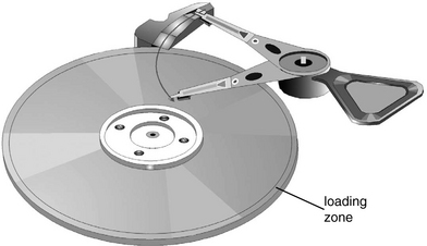
Load/Unload
This technology was previously used in large diameter disk drives and is now being re-introduced into small form factor drives. Prior to spinning down, the actuator moves off the disk platters. A lift tab at the front of the suspension of each HGA slides up a ramp structure and comes to a rest at a detent, as shown in Figure 17.26. The heads are now safely off the disk surfaces, and only then are the disks spun down. To start up the disk drive, the disks are first spun up until a sufficient rotational speed is reached, and then the actuator is moved off the ramp; the heads will have enough air cushion for them to fly as soon as they reach the disk surfaces. With this technique, intentional contact between the head and disk surface is eliminated.
Just as in CSS, a self-parking mechanism is needed to ensure that the heads are safely unloaded up the ramp in the event of a power loss. Again, this can be accomplished by extracting energy from the spinning disks by using a circuit to apply current from the spindle motor back-EMF to the actuator.
Since there is no intentional contact of the head with the disk, reliability of the disk drive is improved as there is less likelihood of head or media damage. It also means the drive can handle more stop/start cycles in its lifetime than CSS. Additionally, because the heads are completely moved off the surfaces of the disks, the whole disk drive is more shock tolerant than drives using CSS. This makes load/unload especially attractive for mobile applications. The downside of load/unload is that it requires a loading zone on each disk surface outside the OD for the head to load onto the disk surface, and no data is stored in this loading zone. This loading zone takes up a lot more space than the landing zone of CSS, which is at the outside of the ID.
17.2.8 Magnetic Disk Recording Integration
One of the most important parameters of a disk drive is its areal recording density. Not only does a high areal density lower the cost per byte of storage, it also has profound impact on performance (discussed in Chapter 19, “Performance Issues and Design Trade-Offs”). All the components of a disk drive described in the previous sections and the way they interact with each other affect the areal density realized in the final integrated product. Of these, the head and the media carry the most weight.
Areal density is the product of two disk drive parameters, namely tpi and bpi. We will examine these two parameters separately and take a high-level overview of how the drive components affect them. As we shall see, miniaturization of the drive components is the key for increasing areal density. Most fortunately, miniaturization to gain higher areal density also results in better performance: smaller heads and lighter actuators enable faster seek, and smaller diameter and thinner disk platters enable higher rotational speed.
Tracks per Inch
As discussed in Section 17.2.3 and stated in Equation 17.6, tpi is the reciprocal of the track pitch, which is the distance between the center of two adjacent tracks. The track width accounts for much of the track pitch, and the track width is basically dictated by the width of the pole tip of the inductive write head. Hence, the width of the write head is a key factor in determining tpi.
While the head may be able to write very narrow tracks, other components of the disk drive must also be able to support a high tpi. The actuator and the servo system controlling it need to be able to both position the head accurately on the center of a track and maintain this centered position while the head is accessing the data on the track. In addition, while the guard bands on both sides of a track allow for a small amount of deviation, such deviation must be kept small. If a normal distribution is assumed for the position of the head with respect to the track center, a value of 3 sigma (representing a range with 99.7% probability) is designated as the TMR of the drive. Clearly, as track pitch decreases, TMR must decrease proportionally if the head is to write and read data properly. NRRO of the spindle motor (discussed previously), mechanical vibrations coming from sources both inside the disk drive and external to the disk drive (e.g., another neighboring disk drive), disk flutter, and even electronic noise in the servo control circuits all contribute to TMR.
Bits per Inch
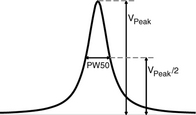
The linear recording density bpi is predominantly determined by the head and the media. As given by Equation 17.8, bpi is inversely proportional to the distance B between two back-to-back transitions. Thus, bpi depends on how closely transitions can be placed one after the other. The ability to place two transitions closely without the detected pulse signals from them (Figure 17.16) overly interfering with each other6 depends on the width of each pulse—the narrower the pulse width the better. The standard measure of pulse width in magnetic recording is the half width, called PW50, which is measured at the 50% amplitude (see Figure 17.27).
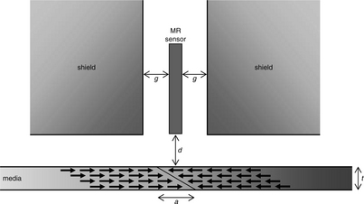
Without derivation here, a number of analytical studies have shown that PW50 can be approximately represented by
where a is the transition parameter (transition length), d is the magnetic separation, g is the half gap in MR head (or pole gap in inductive head), and t is the thickness of media (as shown in Figure 17.28). It should be noted that the magnetic separation d is not the same as the flying height of the slider. Magnetic separation is the spacing between the tip of the sensor and the top of the recording media; so it includes the flying height, and the thickness of the lubricant, and the thickness of the carbon overcoat (on both the media and the sensor).
The transition parameter a can be approximately modelled with the following equation:
where Mr and Hc are the remanent magnetization and coercivity of the medium, respectively, and K is some constant. From Equation 17.9, it can be seen that PW50 can be decreased (which means bpi can be increased) by reducing the MR sensor gap g (miniaturizing the head), the magnetic separation d (lowering the flying height which is the major component), the thickness of the media t, and the transition parameter a. Furthermore, according to Equation 17.10, the transition length a itself can also be shortened by reducing d and t. Selecting a medium material with high coercivity will also help to reduce a, but it requires more current in the inductive head for writing. While a medium with low remanence will also help to make the transition parameter small, it must produce a sufficient magnetic field for the read sensor to detect.
Because reducing the magnetic separation is one of the most significant factors in increasing areal density, flying height has continuously been decreasing over the years. When the RAMAC 350 was first in troduced in 1956, the head-disk separation was 800 microinches. Today, the flying height of a typical disk drive is well below 1 microinch. To put things in perspective, the thickness of human hair is about 3000 microinches, and the size of a typical dust particle is about 1500 microinches.
Tribology
Tribology7 is the study of interaction of surfaces in relative motion, in this case between the head slider and the disk. While tribology is of great importance for CSS, even during the normal flying of the head, interactions between the slider and the disk surface can still occur. This is because asperities on a disk surface are inevitable and can result in contact with the head. Hence, tribology is an important aspect of disk drive design, even for drives using the load/unload technology which theoretically eliminates all intentional contact between the head and the disk. In addition to potentially causing wear due to physical abrasion (which, in turn, can also create contaminants), contact of the head with asperities on a disk surface raises the temperature of the MR head, resulting in temporarily changing its resistance. This phenomenon, known as thermal asperity, manifests itself as severe noise in the read signal. Thus, a high enough flying height is needed to avoid the surface asperities. Unfortunately, a higher flying height is not good for areal density, as discussed previously. This is why tribology is so important in disk drive design, as it holds the key to how low the head can fly over the media and hence dictates what areal density can be achieved. Surface texture, overcoat material, and lubricant material are all part of the tribology domain.
17.2.9 Head-Disk Assembly
All the foregoing physical components described in this section are assembled together to form a head-disk assembly (HDA). It basically includes all the major components of a disk drive except for most of the electronics. The only electronics that is part of the HDA is the small AEM which is integrated with the flex cable. As discussed previously, the size of a dust particle is thousands of times greater than the head’s flying height. With the surface of the disk traveling at over 100 mph past the head, a collision of the head with any contaminant can result in damage to either the head or the recording media. Therefore, assembling the HDA is done inside a clean room. The HDA is mounted inside a housing which is then sealed to keep contaminants out. However, the compartment is not airtight. Rather, air exchange with the outside is allowed through a breather filter so that the drive can adjust to the outside air pressure.8 To capture any contaminants that may come off the HDA after the drive leaves the assembly line, a recirculation filter can also be found inside the HDA compartment.
17.3 Electronics
The remaining physical components of a disk drive are the electronics that control its operation. Except for the AEM, they are located outside the sealed HDA compartment. Due to a high degree of integration, today’s disk drive electronics are reduced to basically a handful of Integrated Circuit (IC) chips which all fit on a small printed circuit board. Figure 17.29 shows the major functional electronic components. The chip boundaries are deliberately not drawn as they may evolve as drive electronics technology changes. In this section, a high-level description of the functions of these components and their sub-components will be described. ICs performing some of these functions are available from several companies and are constantly being refreshed.

17.3.1 Controller
The controller is the brain of the disk drive. It either performs a disk drive function itself directly, or it makes sure that the function gets performed correctly by one of the other components. Figure 17.30 is a high-level block diagram of a controller’s major sub-components. Some of the major functions handled by the controller are the following:

FIGURE 17.30 Block diagram of the controller. The dashed outline indicates functional boundary, not chip boundary.
• Receive commands (I/O requests) from the user, schedule the execution of the commands, and report to the user when a command is completed
• Interface with the HDA, including telling it where to seek to and which sectors to read or write
• Error recovery and fault management
• Starting up and shutting down the disk drive
Processor—A microprocessor is commonly used to execute the above list of functions and to carry out any related computations. The speed with which those functions can be performed not only depends on the speed and power of the microprocessor, but also on how much of a particular function is automated with hardware by one of the other sub-components. For instance, cache function can be completely handled by the processor firmware, or it can be fully or partially automated as part of the memory controller.
ROM—The executable code of the microprocessor resides here. Optionally, only the boot code for the processor is stored here, with the remainder of the controller code read in from a reserved area in the disk. During development of the disk drive, E2PROM can be used instead. Executable code may be copied to SRAM for faster access by the processor.
Memory Controller—This can be as simple as just an interface to some DRAM, or it can include a cache manager performing cache space allocation and cache lookup. Cache is an important subject and will be covered in Chapter 22, “The Cache Layer.”
Host Interface—This is the physical link of the disk drive to the host system it is attached to. It provides the necessary interface hardware (such as specific registers), performs the handshakes of the interface’s protocol, and exchanges data with the user over this link. The host-disk interface will be discussed in greater detail in Chapter 20, “Drive Interface.”
Data Formatter—Its function is to move the data from the memory, partition it into sector size chunks, and route it to the ECC and CRC logic.
ECC and CRC Encoder/Decoder—Error correcting code (ECC) and cyclic redundancy checksum (CRC) are added to each sector of data to be stored together in the media. They are used to provide data integrity and fault tolerance. More detail will be covered in Chapter 18, “The Data Layer.”
17.3.2 Memory
The memory in the disk drive is used mainly to serve three distinct purposes:
1. Part of the memory is used as a scratch-pad for the controller. Each time the drive is powered up, it loads from protected areas in the disk operational tables and parameters onto the memory. Examples include the zoning table (discussed in Chapter 18) which is generally the same for all the drives of a given model, defect maps and no-ID tables (both discussed in Chapter 18) which are drive specific, and various parameters (many of them related to the operation of each individual head) that were self-calibrated during final manufacture testing. Memory is also used for run-time applications, such as for storing the queue of commands received from the host system.
2. The media data transfer rate is different from the data rate of the interface of the disk drive. Part of the memory is used for the purpose of speed-matching between these two different data rates. For instance, during a write operation, data from the host must be buffered in the memory and streamed out to the write channel at the media data rate. For a read operation, data from the media can be temporarily stored in the buffer memory even if the host or the drive interface happens to be busy. Without a buffer, write data may not be available, and read data may have no place to go right at the particular moment the head is ready to write or read that piece of data. The drive will then have to wait for one full disk revolution before it can attempt the same data access again, a condition commonly referred to as “missed rev.” The buffer is therefore essential in eliminating, or at least greatly reducing the number of, such performance-robbing missed revs.
3. Today’s disk drives all have some memory for cache. Caching is an important aspect of disk drive performance and will be treated separately in Chapter 22.
While buffering and caching are two distinct functions, the address space of cache is usually also used for buffering. Today, DRAM is typically used for cache/buffer memory. Non-time-critical data or tables are also stored in DRAM. Tables needed for time-critical functions, such as address translation, are stored in SRAM for faster access by the processor which has dedicated access, unlike DRAM in which the processor has to share access with other hardware. In the future, if newer and better semiconductor memory technology comes along, it may be adopted in the disk drive to replace DRAM or SRAM.
17.3.3 Recording Channel
The read/write recording channel is a critical component of the disk drive which works hand in glove with the head and media to deliver the ultimate linear bit density of the drive. While improvements in heads and media oftentimes get credited for the high growth rate in recording density, advancements in channel technology have actually also contributed substantially. The recording channel controls the placing of user data onto the media (as described earlier in Section 17.2.3) by applying the right polarity of voltage to the inductive write head (hence controlling the direction of current flow in the coil) at the right time and retrieves previously recorded data by interpreting the voltage signal presented by the read sensor. Control signals received from the controller include whether to enable the write circuitry or the read circuitry and a selection of which head to turn on.
The AEM is actually part of the read/write channel. Because the signals to and from (especially from) the heads are small, the write drivers and read preamplifiers are placed in the AEM and located as close to the heads as possible so as to minimize resistance and inductance in the circuit. Hence, sub-components of the AEM are described here as part of the recording channel, even though physically AEM is separated and placed inside the HDA.
Write Channel
The write channel is the set of circuits that transforms the user data from its binary logic format into actual currents being sent to the write head. When writing data, the write channel supplies current to the write head, reversing the direction of current flow whenever a magnetic transition is to be created in the media. However, the 1’s and 0’s of user’s data are not directly recorded as is. Rather, some modulation code is employed to ensure that the sequence of bits recorded and later retrieved satisfies certain desirable properties. Such properties include the following:
• Because the clocking for the reading of data is extracted from the recorded data bits, a very long string of 0’s would mean there is no transition and hence no clocking information. This can lead to read errors as the clock can drift if it is not resynchronized for an extended period. Thus, it is necessary to limit the maximum length of run of 0’s.
• If an error occurs in reading one bit, propagation of its effect must be well contained so that it does not turn into a long burst of errors.
• Have a high density ratio (DR) of data bits per flux change. This directly affects bpi, as indicated in Equation 17.8.
The coding method of using a transition to represent a 1, as discussed in Section 17.1.5, is known as nonreturn to zero inverted (NRZI) encoding. NRZI encoding places no limit on the number of consecutive 0’s that can appear. One of the earliest methods introduced to prevent long runs of 0’s in recorded signal is the FM (frequency modulation) encoding. In this scheme, a 1 is simply inserted after every data bit. For example, the data sequence 10001 would be encoded as 1101010111. FM is a rather poor encoding technique as the coding efficiency is only 50%. A slightly improved modified frequency modulation (MFM) scheme is to encode 1 into 01, while a 0 is encoded into10 if the preceding bit is 0 and into 00 if the preceding bit is 1. Hence, the sample sequence of 10001 would be encoded as 0100101001. While the code rate for MFM is still only 50%, because two 1’s are separated by at least one 0, higher recording density can be achieved (assuming recording density is limited by the minimum distance between two transitions).
Modulation coding has gone through several major changes and many evolutionary changes over the years. FM and MFM are actually special cases of run-length-limited (RLL) codes. RLL code is specified as m/n(d,k), where m is the number of data bits encoded into n code bits, d is the minimum number of 0’s required between two 1’s, and k is the maximum number of 0’s allowed. Thus, FM is a 1/2(0,1) RLL code, and MFM is a 1/2(1,2) RLL code. The DR is given by
For example, the 8/9(0,4) RLL code has a DR of 8/9, which makes the achievable bpi with that code 0.89 that of the fcpi of what the head-disk technology can deliver. Newer and more efficient codes have been developed in recent years, and multiple choices are oftentimes offered by suppliers of channel chips for disk drive designers to select the one that meets their needs.
The k parameter of RLL code is determined by how long the clocking can go without resync. The d parameter is a function of how well the channel can handle inter-symbol interference. Inter-symbol interference (ISI) occurs when the transitions are packed so close together that the detectable signal from a transition is distorted by those of its neighboring transitions. The pattern of ISI depends on the particular recorded bit sequence.
The simplest example would be of two 1’s in the midst of a string of 0’s. Figure 17.31(a) shows that when the two transitions are placed far enough apart, there is no interference of one pulse with the other. When the two transitions are packed closer together to increase bpi, the two pulses start to cancel each other. As a result, the amplitudes of the two pulses are reduced, and, more importantly, their peaks are shifted, as shown in Figure 17.31(b). The first peak arrives early, while the second peak arrives late. As the read process of today’s disk drives is done synchronously based on a fixed clock rate, a shift causes the peak to be out of step with the clock signal and can potentially lead to read error. Since ISI is the unavoidable result of packing transitions more densely in order to increase bpi, multiple techniques have been developed to deal with ISI. One such technique is to precompensate the write signal delivered to the write driver. For the simple peak shift example of the double transitions, precompensation would delay the first transition and move up the second transition. Write precompensation is sometimes referred to as write equalization.
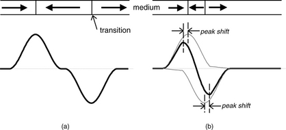
FIGURE 17.31 An example of ISI: (a) two transitions spaced far apart—no ISI; (b) two transitions placed close together—peak shift results.
Figure 17.32 is a functional block diagram of the sub-components of a write channel. The write driver, by means of a simple flip-flop circuit, uses a current source to apply a voltage of the right polarity, in accordance to the write signal provided by the write precompensation circuit, to the inductive write head.
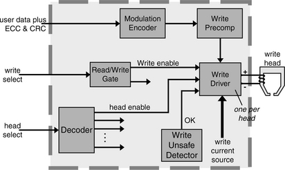
However, before it can do that, the write driver must be enabled by three control signals:
1. The controller must first signal that it wants to do a write to the read/write gate.
2. The controller needs to determine which of the heads is to do the write and tells the decoder to enable that head.
3. There is a circuit which detects any condition which makes it unsafe to write, such as the head is not over the right track. This circuit must signal that it is okay to write.
All three conditions must be met all the time during the write for the write driver to apply current to the head.
Read Channel
The read channel is a series of circuits that converts the analog signals sensed by the read head back into the original user data in their binary logic format. Figure 17.33 shows a block diagram of the major components of a typical read channel. With today’s microscopic bit size, the signal picked up by the GMR head is very small, well below 1 mV. The first order of business is to greatly amplify this signal as soon as possible before it picks up more noise. This is handled by the preamp which is a differential amplifier located in the AEM. For the preamp of a read head to go active, the controller must first signal that it wants to do a read to the read/write selector, and the head must also be selected by the decoder based on the controller’s selection of which head to use. When enabled, the selected head’s AEM module applies a sensing current to its MR sensor.
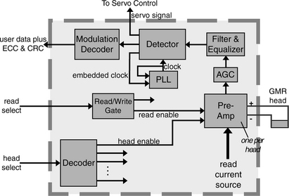
The amplified signal from the AEM is passed on to an automatic gain control (AGC) circuit to adjust the peak voltages of the signal to within the range required by subsequent circuitries. A low-pass filter following the AGC reduces high-frequency noise. The equalizer is a circuit which slims the pulses, that is, makes the shape of the pulses narrower. This is another technique employed to combat ISI, in addition to write precompensation described previously.
The conditioned signal is now ready for the detection circuit. The detector extracts servo information (see Section 17.3.4 and Chapter 18), as well as the original recorded binary information. Servo information is fed to the actuator servo control circuit. Encoded user data is written to the disk synchronously using a clocking signal. Hence, to extract data accurately from the read-back signal, the detector must also extract the clocking information embedded with the data. The extracted clock signal is fed to a phase-locked loop (PLL) circuit to regulate the clock that the detector uses to recover data. While the frequency of the clock is adjusted gradually based on the average of several bits, adjustment for individual data pulse timing is immediate and based only on the current detected clock pulse.
Earlier disk drives used peak detection to directly look for pulses created by transitions in the media. With this technique, the pulse signal is differentiated, and the detection logic looks for zero-crossing of the differentiated output as where a peak has occurred. In 1990, the IBM 0681 disk drive introduced PRML (partial response maximum likelihood) as a new method for data recovery. While known to the data communication field for a long time, PRML was a breakthrough technology for magnetic recording. It is a very effective technique for dealing with ISI and permits denser packing of transitions than peak detection. There are two key aspects to PRML. First, the signal is sampled, which is called a partial response signal. Second, instead of decoding each pulse individually as in peak detection, it decodes a short sequence of bits in a sliding window. For each sequence of sampled signal, it looks for the bit sequence which is most likely (hence, maximum likelihood) to generate that sampled sequence.
Regardless of the data detection method used, the last stage of a read channel is to run the data output of the detector through a modulation code decoder to recover the original user data and ECC/CRC information.
17.3.4 Motor Controls
The spindle motor and the actuator VCM are two different types of electric motors with two distinct forms of motion to perform two very different mechanical functions. One is to spin the disk platters at a constant rotational speed. The other is to move the actuator so as to place the active head at a radial position very precisely. Yet, the desired motion of both can be controlled by governing the current (amplitude and direction) being applied to the motor. Both use a feedback loop for control by constantly monitoring the status of the motor and sending the information to the control logic. The control logic then computes the amount of correction that is needed and adjusts the current output to the motor accordingly.
Figure 17.34 shows a high-level schematic of the actuator servo control system and how the logic flows [Chen et al. 2006, Oswald 1974]. The key of the servo system is that special servo patterns are written on the disks at manufacturing time. These servo patterns provide precise information of their location. Detailed descriptions of the servo patterns are covered in Chapter 18. The read channel detects these servo patterns and forwards the signals from these patterns to a decoding circuit which decodes the signals into positional information. The positional information is fed to the servo control logic which compares it with the target track position requested by the disk drive’s controller. The difference is used to generate a corrective action signal, which is fed to the VCM driver for adjusting the current that is being applied to the VCM. This closed-loop logic flow takes place continuously as long as the drive is active, whether it is seeking a new location or following a track to keep the head centered over it. Earlier drives used analog circuits to perform the servo control functions. Today, the job is being handled by a digital signal processor (DSP), which means the servo control includes an analog to digital converter (ADC) for converting the analog servo signals to digital form and a digital to analog converter (DAC) for converting the digital correction signal into analog input for the power amplifier of the VCM driver.
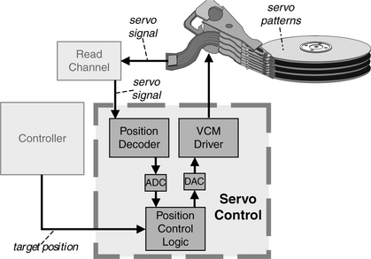
The spindle motor is also controlled using a feedback loop. Here, the motor status information being fed back to its control circuit is simply its rotational speed. Some earlier disk drives used Hall sensors to measure the motor speed. Today’s disk drives determine the motor’s rotational speed by measuring the back-EMF voltage from the motor coil generated by the spinning motor.
1TMR is the amount of offset between the center of the head and the center of the written track.
2Biasing is a long topic beyond the scope of this book. The choice of biasing scheme needs to trade off between maximizing signal amplitude and minimizing signal asymmetry.
3Called the “exchange layer.”
4Actually, with improving protective overcoats for both the head and the media, better lubricants, and the constant pressure to reduce flying height in order to increase areal density, contact recording is now again a subject of discussion and investigation. To achieve practical contact recording, a tougher disk overcoat needs to be engineered, and lubricants that can be used as liquid bearings will have to be developed.
5Even though the configuration of the coil and magnets here is completely different from that of a cone speaker, the term “voice coil motor” sticks.
6Current channel technology can handle a small degree of inter-symbol interference.
7“Tribo” comes from Greek meaning “friction.”
8Special disk drives for high altitude and space applications are exceptions. They have to be truly sealed to keep the air from leaking out since the heads must have air to fly.