
Storage Subsystems
Up to this point, the discussions in Part III of this book have been on the disk drive as an individual storage device and how it is directly connected to a host system. This direct attach storage (DAS) paradigm dates back to the early days of mainframe computing, when disk drives were located close to the CPU and cabled directly to the computer system via some control circuits. This simple model of disk drive usage and configuration remained unchanged through the introduction of, first, the mini computers and then the personal computers. Indeed, even today the majority of disk drives shipped in the industry are targeted for systems having such a configuration.
However, this simplistic view of the relationship between the disk drive and the host system does not tell the whole story for today’s higher end computing environment. Sometime around the 1990s, computing evolved from being computation-centric to storage-centric. The motto is: “He who holds the data holds the answer.” Global commerce, fueled by explosive growth in the use of the Internet, demands 24/7 access to an ever-increasing amount of data. The decentralization of departmental computing into networked individual workstations requires efficient sharing of data. Storage subsystems, basically a collection of disk drives, and perhaps some other backup storage devices such as tape and optical disks, that can be managed together, evolved out of necessity. The management software can either be run in the host computer itself or may reside in a dedicated processing unit serving as the storage controller. In this chapter, welcome to the alphabet soup world of storage subsystems, with acronyms like DAS, NAS, SAN, iSCSI, JBOD, RAID, MAID, etc.
There are two orthogonal aspects of storage subsystems to be discussed here. One aspect has to do with how multiple drives within a subsystem can be organized together, cooperatively, for better reliability and performance. This is discussed in Sections 24.1-24.3. A second aspect deals with how a storage subsystem is connected to its clients and accessed. Some form of networking is usually involved. This is discussed in Sections 24.4-24.6. A storage subsystem can be designed to have any organization and use any of the connection methods discussed in this chapter. Organization details are usually made transparent to user applications by the storage subsystem presenting one or more virtual disk images, which logically look like disk drives to the users. This is easy to do because logically a disk is no more than a drive ID and a logical address space associated with it. The storage subsystem software understands what organization is being used and knows how to map the logical addresses of the virtual disk to the addresses of the underlying physical devices. This concept is described as virtualization in the storage community.
24.1 Data Striping
When a set of disk drives are co-located, such as all being mounted in the same rack, solely for the purpose of sharing physical resources such as power and cooling, there is no logical relationship between the drives. Each drive retains its own identity, and to the user it exhibits the same behavioral characteristics as those discussed in previous chapters. A term has been coined to describe this type of storage subsystems—JBOD, for just-a-bunch of disks. There is nothing more to be said about JBOD in the remainder of this chapter.
The simplest organizational relationship that can be established for a set of drives is that of data striping. With data striping, a set of K drives are ganged together to form a data striping group or data striping array, and K is referred to as the stripe width. The data striping group is a logical entity whose logical address space is sectioned into fixed-sized blocks called stripe units. The size of a stripe unit is called the stripe size and is usually specifiable in most storage subsystems by the administrator setting up the stripe array. These stripe units are assigned to the drives in the striping array in a round-robin fashion. This way, if a user’s file is larger than the stripe size, it will be broken up and stored in multiple drives. Figure 24.1 illustrates how four user files of different sizes are stored in a striping array of width 3. File e takes up four stripe units and spans all three disks of the array, with Disk 1 holding two units, while Disks 2 and 3 hold one unit each. File f continues with seven stripe units and also spans all three disks with multiple stripe units in each disk. File g is a small file requiring only one stripe unit and is all contained in one disk. File h is a medium size file and spans two of the three disks in the array.

FIGURE 24.1 An example of a data striping array with a stripe width = 3. Four user files e, f, g, and h of different sizes are shown.
The purpose of data striping is to improve performance. The initial intent for introducing striping was so that data could be transferred in parallel to/from multiple drives, thus cutting down data transfer time. Clearly, this makes sense only if the amount of data transfer is large. To access the drives in parallel, all drives involved must perform a seek operation and take a rotational latency overhead. Assuming the cylinder positions of all the arms are roughly in sync, the seek times for all drives are about the same. However, since most arrays do not synchronize the rotation of their disks,1 the average rotational latency for the last drive out of K drives to be ready is R × K/(K + 1), where R is the time for one disk revolution. This is higher than the latency of R/2 for a single drive. Let FS be the number of sectors of a file. The I/O completion time without data striping is2
where SPT is the number of sectors per track. When data striping is used, the I/O time is
seek time + R × K/(K + 1) + FS × R/K × SPT (EQ 24.2)
Assuming the seek times are the same in both cases, data striping is faster than non-striping when
R/2 + f × R/SPT > R × K/(K + 1) + f × R/K × SPT (EQ 24.3)
f > K × SPT/2(K + 1) (EQ 24.4)
Thus, the stripe size should be chosen to be at least SPT/2(K + 1) sectors in size3 so that smaller files do not end up being striped.
That, however, is only part of the story. With striping, all the drives are tied up servicing a single command. Furthermore, the seek and rotational latency overhead of one command must be paid by every one of the drives involved. In other words, the overhead is paid for K times. On the other hand, if striping is not used, then each drive can be servicing a different command. The seek and latency overhead of each command are paid for by only one disk, i.e., one time only. Thus, no matter what the stripe size and the request size are, data striping will never have a better total throughput for the storage subsystem as a whole when compared to non-striping. In the simplest case where all commands are of the same size f, the throughput for data striping is inversely proportional to Equation 24.1, while that for non-striping is inversely proportional to Equation 24.2 times K. Only when both seek time and rotational latency are zero, as in sequential access, can the two be equal. Thus, as long as there are multiple I/Os that can keep individual disks busy, parallel transfer offers no throughput advantage. If the host system has only a single stream of long sequential accesses as its workload, then data striping would be a good solution for providing a faster response time.
This brings up another point. As just discussed, parallel data transfer, which was the original intent of data striping, is not as effective as it sounds for improving performance in the general case. However, data striping is effective in improving performance in general because of a completely different dynamic: its tendency to evenly distribute I/O requests to all the drives in a subsystem. Without data striping, a logical volume will be mapped to a physical drive. The files for each user of a storage subsystem would then likely end up being all placed in one disk drive. Since not all users are active all the time, this results in what is known as the 80/20 access rule of storage, where at any moment in time 80% of all I/Os are for 20% of the disk drives, which means the remaining 80% of the disk drives receive only 20% of the I/Os. In other words, a small fraction of the drives in the subsystem is heavily utilized, while most other drives are lightly used. Users of the heavily utilized drives, who are the majority of active users at the time, would experience slow response times due to long queueing delays,4 even though many other drives are sitting idle. With data striping, due to the way logical address space is spread among the drives, each user’s files are likely to be more or less evenly distributed to all the drives instead of all concentrated in one drive. As a result, the workload to a subsystem at any moment in time is likely to be roughly divided evenly among all the drives. It is this elimination of hot drives in a storage subsystem that makes data striping a useful strategy for performance improvement when supporting multiple users.
24.2 Data Mirroring
The technique of using data striping as an organization is purely for improving performance. It does not do anything to help a storage subsystem’s reliability. Yet, in many applications and computing environments, high data availability and integrity are very important. The oldest method for providing data reliability is by means of replication. Bell Laboratories was one of the first, if not the first, to use this technique in the electronic switching systems (ESS) that they developed for telephony. Data about customers’ equipment and routing information for phone lines must be available 24/7 for the telephone network to operate. “Dual copy” was the initial terminology used, but later the term “data mirroring” became popularized in the open literature. This is unfortunate because mirroring implies left-to-right reversal, but there definitely is no reversal of bit ordering when a second copy of data is made. Nevertheless, the term is now universally adopted.
Data mirroring provides reliability by maintaining two copies5 of data [Ng 1986, 1987]. To protect against disk drive failures, the two copies are kept on different disk drives.6 The two drives appear as one logical drive with one logical address space to the user. When one drive in a mirrored subsystem fails, its data is available from another drive. At this point the subsystem is vulnerable to data loss should the second drive fail. To restore the subsystem back to a fault-tolerant state, the remaining copy of data needs to be copied to a replacement disk.
In addition to providing much improved data reliability, data mirroring can potentially also improve performance. When a read command requests a piece of data that is mirrored, there is a choice of two places from which this data can be retrieved. This presents an opportunity for some performance improvement. Several different strategies can be applied:
• Send the command to the drive that has the shorter seek distance. For random access, the average seek distance drops from 1/3 of full stroke to 5/24 (for no zone bit recording). This assumes that both drives are available for handling a command. Thus, its disadvantage is that it ties up both drives in servicing a single command, which is not good for throughput.
• Send the read command to both drives and take the data from the first one to complete. This is more effective than the previous approach in cutting the response time for the command, as it minimizes the sum of seek time and rotational latency. It also has the same disadvantage of tying up both drives in servicing a single command.
• Assign read commands to the two drives in a ping-pong fashion so that each drive services half of the commands. Load sharing by two drives improves throughput.
• Let one drive handle commands for the first half of the address space, and the other drive handle commands for the second half of the address space. This permits load sharing, while at the same time reduces the average seek distance to one-sixth of full stroke. However, if the workload is such that address distribution is not even, one drive may become more heavily utilized than the other. Also, a drive may become idle while there is still a queue of commands for the other drive.
• A good strategy is to maintain a single queue of commands for both mirrored disks. Each drive that becomes available fetches another command from the shared queue. In this way, both drives get fully utilized. If RPO could be applied in selecting the next command to fetch, that would be the best strategy.
Mirrored disks have a write penalty in the sense that both drives containing the mirrored data need to be updated. One might argue that this is not really a penalty since there is no increase in workload on a per physical drive basis. If write caching is not on, a write is not complete until both drives have done the write. If both drives start the write command at the same time, the mechanical delay time is the larger of the sum of seek and latency of the two drives. If the drives do not start at the same time, then the delay for the write completion is even longer.
There are different ways that data can be mirrored in a storage subsystem [Thomasian & Blaum 2006]. Three of them are described in the following, followed by discussions on their performance and reliability.
24.2.1 Basic Mirroring
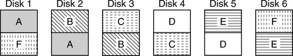
The simplest and most common form of mirroring is that of pairing off two disks so that they both contain exactly the same data image. If M is the number of disk drives in a storage subsystem, then there would be M/2 pairs of mirrored disks; M must be an even number. Figure 24.2 illustrates a storage subsystem with six drives organized into three sets of such mirrored disks. In this and in Figures 24.3 and 24.4 each letter represents logically one-half the content, or logical address space, of a physical drive.


24.2.2 Chained Decluster Mirroring
In this organization, for any one of the M drives in the subsystem, half of its content is replicated on a second disk, while the other half is replicated on a third disk [Hsiao & DeWitt 1993]. This is illustrated in Figure 24.3 for M = 6. In this illustration, half of the replication resides in a drive’s immediate neighbors on both sides. Note that for this configuration, M does not have to be an even number, which makes this approach more flexible than the basic mirroring method.
24.2.3 Interleaved Decluster Mirroring
In this third organization, for any one of the M drives in the subsystem, half of its content is divided evenly into (M – 1) partitions. Each partition is replicated on a different drive. The other half of the content of a drive consists of one partition from each of the other (M – 1) drives. Figure 24.4 illustrates such a subsystem with M = 6 drives. M also does not have to be an even number for this mirroring organization.
24.2.4 Mirroring Performance Comparison
When looking into the performance of a fault-tolerant storage subsystem, there are three operation modes to be considered. When all the drives are working, it is called the normal mode. Degraded mode is when a drive has failed and the subsystem has to make do with the remaining drives to continue servicing user requests. During the time when a replacement disk is being repopulated with data, it is called the rebuild mode.
Normal Mode
One factor that affects the performance of a subsystem is whether data striping is being used. Data striping can be applied on top of mirroring in the obvious way. Figure 24.5 illustrates applying the striping example of Figure 24.1 to basic mirroring. As discussed earlier, one benefit of data striping is that it tends to distribute the workload for a subsystem evenly among the drives. So, if data striping is used, then during normal mode all mirroring organizations have similar performance, as there is no difference in the I/O load among the drives. Any write request must go to two drives, and any read request can be handled by one of two drives.
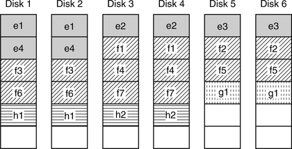
FIGURE 24.5 An example of applying data striping to basic mirroring. Using the example of Figure 24.1, four user files e, f, g, and h are shown.
When data striping is not used, hot data can make a small percentage of mirrored pairs very busy in the basic mirroring organization. For the example illustrated in Figure 24.2, high I/O activities for data in A and B will result in more requests going to Disks 1 and 2. Users of this pair of mirrored drives will experience a longer delay. With chained decluster mirroring, it can be seen in Figure 24.3 that activities for A and B can be handled by three drives instead of two, namely Disks 1, 2, and 3. This is an improvement over basic mirroring. Finally, with interleaved decluster mirroring, things are even better still as all drives may be involved for handling read requests for A and B, even though Disks 1 and 2 must handle more writes than the other drives.
Degraded Mode
During normal mode, a read request for any piece of data can be serviced by one of two possible disks, regardless of which mirroring organization is used. When one drive fails, in basic mirroring all read requests to the failed drive must now be handled by its mate, doubling its load for read. For chained decluster mirroring, the read workload of the failed drive is borne by two drives. For the example of Figure 24.3, if Disk 3 fails, then read requests for data B and C will have to be handled by Disks 2 and 4, respectively. On the surface, the workload for these two drives would seem to be increased by 50%. However, the subsystem controller can divert much of the read workload for D to Disk 5 and much of the workload for A to Disk 1. This action can ripple out to all the remaining good drives in the chained decluster array until every drive receives an equal workload. This can happen only if the array is subject to a balanced workload distribution to begin with, as in data striping. Finally, with interleaved decluster mirroring, reads for the failed drive are naturally shared by all remaining (M – 1) good drives, giving it the best degraded mode performance.
Rebuild Mode
A similar situation exists in degraded mode. In addition to handling normal user commands, the mirrored data must be read in order for it to be rewritten onto the replacement drive. In basic mirroring, all data must come from the failed drive’s mate, adding even more workload to its already doubled read workload. With chained decluster mirroring, half of the mirrored data comes from one drive, while the other half comes from another drive. For interleaved decluster mirroring, each of the (M – 1) remaining good drives is responsible for doing the rebuild read of 1/(M – 1)th of the mirrored data.
In summary, of the three different organizations, basic mirroring provides the worst performance, especially during degraded and rebuild modes. Interleaved decluster mirroring has the most balanced and graceful degradation in performance when a drive has failed, with chained decluster mirroring performing between the other two organizations.
24.2.5 Mirroring Reliability Comparison
For a user, a storage subsystem has failed if it loses any of his data. Any mirroring organization can tolerate a single drive failure, since another copy of the failed drive’s data is available elsewhere. Repair entails replacing the failed drive with a good drive and copying the mirrored data from the other good drive, or drives, to the replacement drive. When a subsystem has M drives, there are M ways to have the first disk failure. This is where the similarity ends. Whether a second drive failure before the repair is completed will cause data loss depends on the organization and which drive is the second one to fail out of the remaining (M – 1) drives [Thomasian & Blaum 2006].
Basic Mirroring
With this organization, the data of a drive is replicated all on a second drive. Thus, only if this second drive fails will the subsystem suffer a data loss. In other words, there is only one failure out of (M – 1) possible second failures that will cause data loss. The mean time to data loss (MTTDL) for an M disk basic mirroring subsystem is approximately
where MTTF is the mean time to failure for a disk, and MTTR is the mean time to repair (replace failed drive and copy data). This is assuming that both failure and repair are exponentially distributed.
Chained Decluster Mirroring
With this organization, the data of a drive is replicated onto two other drives. Thus, if either of these two drives also fails, the subsystem will suffer data loss, even though half and not all of the data of a drive is going to be lost. In other words, there are two possible second failures out of (M – 1) possible failures that will cause data loss. The MTTDL for an M disk chained decluster mirroring subsystem is approximately
Interleaved Decluster Mirroring
With this organization, the data of a drive is replicated onto all the other drives in the subsystem. Thus, if any one of these (M – 1) drives fails, the subsystem will suffer data loss, even though 1/(M – 1)th and not all of the data of a drive is going to be lost. The MTTDL for an M disk interleaved decluster mirroring subsystem is approximately
which is (M – 1) times worse than that for basic mirroring.
In summary, interleave decluster mirroring has the lowest reliability of the three organizations, while basic mirroring has the highest; chained decluster in between these two. This ordering is exactly the reverse of that for performance. Thus, which mirroring organization to use in a subsystem is a performance versus reliability trade-off.
24.3 RAID
While data replication is an effective and simple means for providing high reliability, it is also an expensive solution because the number of disks required is doubled. A different approach that applies the technique of error correcting coding (ECC), where a small addition in redundancy provides fault protection for a larger amount of information, would be less costly. When one drive in a set of drives fails, which drive has failed is readily known. In ECC theory parlance, an error whose location is known is called an erasure. Erasure codes are simpler than ECCs for errors whose locations are not known. The simplest erasure code is that of adding a single parity bit. The parity P for information bits or data bits, say, A, B, C, D, and E, is simply the binary exclusive-OR of those bits:
A missing information bit, say, B, can be recovered by XORing the parity bit with the remaining good information bits, since Equation 24.8 can be rearranged to
The application of this simple approach to a set of disk drives was first introduced by Ken Ouchi of IBM with a U.S. patent issued in 1978 [Ouchi 1978].
A group of UC Berkeley researchers in 1988 coined the term redundant array of inexpensive drives7(RAID) [Patterson et al. 1988] and created an organized taxonomy to different schemes for providing fault tolerance in a collection of disk drives. This was quickly adopted universally as standard, much to the benefit of the storage industry. In fact, a RAID Advisory Board was created within the storage industry to promote and standardize the concept.
24.3.1 RAID Levels
The original Berkeley paper, now a classic, enumerated five classes of RAID, named Levels8 1 to 5. Others have since tacked on additional levels. These different levels of RAID are briefly reviewed here [Chen et al. 1988].
RAID-0
This is simply data striping, as discussed in Section 4.1. Since data striping by itself involves no redundancy, calling this RAID-0 is actually a misnomer. However, marketing hype by storage subsystem vendors, eager to use the “RAID” label in their product brochures, has succeeded in making this terminology generally accepted, even by the RAID Advisory Board.
RAID-1
This is the same as basic mirroring. While this is the most costly solution to achieve higher reliability in terms of percentage of redundancy drives required, it is also the simplest to implement. In the early 1990s, EMC was able to get to the nascent market for high-reliability storage subsystem first with products based on this simple approach and had much success with it.
When data striping, or RAID-0, is applied on top of RAID-1, as illustrated in Figure 24.5, the resulting array is oftentimes referred to as RAID-10.
RAID-2
In RAID-2, fault tolerance is achieved by applying ECC across a set of drives. As an example, if a (7,4)9 Hamming code is used, three redundant drives are added to every four data drives. A user’s data is striped across the four data drives at the bit level, i.e., striping size is one bit. Corresponding bits from the data drives are used to calculate three ECC bits, with each bit going into one of the redundant drives. Reads and writes, even for a single sector’s worth of data, must be done in parallel to all the drives due to the bit-level striping. The RAID-2 concept was first disclosed by Michelle Kim in a 1986 paper. She also suggested synchronizing the rotation of all the striped disks.
RAID-2 is also a rather costly solution for achieving higher reliability. It is more complex than mirroring and yet does not have the flexibility of mirroring. It never was adopted by the storage industry since RAID-3 is a similar but simpler and less costly solution.
RAID-3
This organization concept is similar to RAID-2 in that bit-level striping10 is used. However, instead of using Hamming ECC code to provide error correction capability, it uses the simple parity scheme discussed previously to provide single drive failure (erasure) fault tolerance. Thus, only one redundant drive, called the parity drive, needs to be added, regardless of the number of data drives. Its low overhead and simplicity makes RAID-3 an attractive solution for designing a high-reliability storage subsystem. Because its data access is inherently parallel due to byte-level striping, this architecture is suitable for applications that mostly transfer a large volume of data. Hence, it is quite popular with supercomputers. Since the drives cannot be individually accessed to provide high IOPS for small block data accesses, it is not a good storage subsystem solution for on-line transaction processing (OLTP) and other database-type applications.
RAID-4
This architecture recognizes the shortcoming of the lack of individual disk access in RAID-3. While retaining the use of single parity to provide for fault tolerance, it disassociates the concept of data striping from parity striping. While each parity byte is still the parity of all the corresponding bytes of the data drives, the user’s data is free to be striped with any striping size. By choosing a striping width that is some multiple of sectors, accessibility of user’s data to individual disks is now possible. In fact, a user’s data does not even have to be striped at all, i.e., striping size can be equal to one disk drive.
RAID-4 is a more flexible architecture than RAID-3. Because of its freedom to choose its data striping size, data for any workload environment can be organized in the best possible optimization allowable under data striping, and yet it enjoys the same reliability as RAID-3. However, this flexibility does come at a price.
In RAID-3, writes are always done in full stripes so that the parity can always be calculated from the new data. With RAID-4, as drives are individually accessible, a write request may only be for one of the drives. Take Equation 24.8, and generalize it so that each letter represents a block in one drive. Suppose a write command wants to change block C to C’. Because blocks A, B, D, and E are not changed and therefore not sent by the host as part of the write command, the new parity P’,
cannot be computed from the command itself. One way to generate this new parity is to read the data blocks A, B, D, and E from their respective drives and then XOR them with the new data C’. This means that the write command in this example triggers four read commands before P’ can be calculated and C’ and P’ can be finally written. In general, if the total number of data and parity drives is N, then a single small write command to a RAID-4 array becomes (N – 2) read commands and two write commands for the underlying drives.
It can be observed that when Equations 24.8 and 24.10 are combined, the following equation results:
Therefore, an alternative method is to read the original data block C and the original parity block P, compute the new parity P’ in accordance with Equation 24.12, and then write the new C’ and P’ back to those two drives. Thus, a single, small write command becomes two read-modify-write (RMW) commands, one to the target data drive and one to the parity drive. The I/O completion time for a RMW command is the I/O time for a read plus one disk revolution time.
Either method adds a lot of extra disk activities for a single, small write command. This is often referred to as the small write penalty. For N > 3, which is usually the case, the second method involving RMW is more preferable since it affects two drives instead of all N drives, even though RMW commands take longer than regular commands.
RAID-5
With RAID-4, parity information is stored in one dedicated parity drive. Because of the small write penalty, the parity drive will become a bottleneck for any workload that has some amount of small writes, as it is involved in such writes for any of the data drives. Also, for a heavily read workload, the parity drive is underutilized. The Berkeley team recognized this unbalanced distribution of workload and devised the RAID-5 scheme as a solution.
RAID-5 uses an organization which is very similar to that of data striping. The address space of each disk drive in the group is partitioned into fixed-size blocks referred to as parity stripe blocks, and the size is called the parity stripe block size. The corresponding blocks from each disk together form a parity group. The number of disks in a parity group is referred to as the parity group width. Each parity group includes N data blocks and one parity block.11 Finally, the parity blocks from different parity groups are distributed evenly among all the drives in the array. Figure 24.6 illustrates an example of a 6-disk RAID-5 with the placement of the parity blocks Pi rotated among all the drives. Note that Figure 24.6 is only a template for data placement, and the pattern can be repeated as many times as necessary depending of the parity stripe block size. For example, if drives with 60 GB are used here, and the block size is chosen to be 1 MB, then the pattern will be repeated 10,000 times.

FIGURE 24.6 An example of RAID-5 with 6 disks (5 + P). Parity block Pi is the parity of the corresponding Di data blocks from the other disks.
As it is possible to access individual disk drives, RAID-5 has the same small block write penalty of RAID-4. However, since parity blocks are evenly distributed among all the drives in an array, the bottleneck problem associated with the dedicated parity drive of RAID-4 is eliminated. Because of this advantage of RAID-5, and everything else being equal, RAID-4 is not used in any storage subsystems.
The parity stripe block size does not have to be the same as the data stripe size. In fact, there is no requirement that data striping needs to be used in RAID-5 at all. Figure 24.7 illustrates how the example of data striping of Figure 24.1 can be organized in a 4-disk RAID-5 with the parity stripe block size 2x the data stripe size. While there is no requirement that parity stripe size and data stripe size must be equal, doing so will certainly make things a little easier to manage for the array control software, which needs to map user’s address space to drives’ address spaces while keeping track of where the parity blocks are.

RAID-6
RAID-5 offers a single drive failure protection for the array. If even higher reliability of protection against double drive failures is desired, one more redundancy drive will be needed. The simple bitwise parity across all data blocks schemes is retained for the first redundancy block, but cannot be used for the second redundancy. A more complex coding scheme is required. Furthermore, because updating this second redundancy also requires RMW for small writes, the new redundancy blocks are also distributed among all the drives in the array à la RAID-5. The resulting organization is RAID-6, as illustrated in Figure 24.8 for a 6-disk array.12 Pi is parity of the corresponding Di data blocks in the ith parity group, and Qi is the second redundancy block computed from Dis and Pi.

When one drive in a RAID-6 fails, requests for its content can be reconstructed from the remaining good drives using the simple parity P in exactly the same way as RAID-5. Repair consists of replacing the failed drive and rebuilding its content from the other good drives. If another drive fails before the first failure can be repaired, then both P and the more complicated redundancy Q will be needed for data reconstruction. Some form of Reed-Solomon code was suggested for the second redundancy in the original RAID-6 description. However, Reed-Solomon decoding logic is somewhat complex, and so later on others came up with alternative types of code, such as Even-Odd [Blaum et al. 1995] that uses simple XOR logic for the decoder. Regardless of what code is used, any array with two redundant drives to provide double failure protection can be referred to as RAID-6.
24.3.2 RAID Performance
Mirroring and RAID-4/5/6 have some performance similarity and dissimilarity [Ng 1989, Schwarz & Burkhard 1995]. RAID-3 has different performance characteristics because its component drives cannot be accessed individually. In the following, for ease of discussion, it will be assumed that the workload to an array is normally evenly distributed among all the disks, as in the case with data striping.
Normal Mode Performance
Mirroring has the best normal mode read performance because read requests can be serviced by one of two different drives. RAID-5/6 have the same read performance as that of JBOD, with RAID-4 slightly worse since it has one fewer data drive. RAID-3 has good read performance with large block requests, but the component drives are underutilized when servicing small block requests.
For write requests, RAID-3 performs the same as reads. Both mirroring and RAID-4/5/6 have write penalties. In the case of mirroring, the penalty is that the write must be done to both disks. For RAID-4/5, a small block write request becomes two RMW requests. In the case of RAID-6, a small block write request becomes three RMW requests. For RAID-4/5/6, if a full data stripe is written, there is no penalty since it is not necessary to read the old data. This argues for using a smaller data stripe size to increase the likelihood of writes being full stripe, which is contrary to the discussion on data striping in general in Section 24.1.
This is summarized in Table 24.1 for different arrays with N data disks, or N equivalent data disks. Each array is given a total workload of R reads and W small writes. The table shows the workload as seen by each drive in the array for various organizations. The total number of disks in an array is an indication of its relative cost in providing the equivalent of N disks of storage space. Mirroring has the lightest workload per drive and, therefore, should have the best performance, but it is also the most expensive solution. Not surprisingly, the double-fault-tolerant RAID-6 has a high workload per drive and thus low performance. RAID-3 also has low small block performance.

Degraded Mode and Rebuild Mode Performance
The impact on performance of a disk failure in mirroring depends on which one of the mirroring schemes is used and has been discussed in Section 24.2.4. For RAID-3, performance is not affected by a drive failure since it is always reading in parallel anyway, so the missing data can be reconstructed on the fly. For RAID-4/5, read requests to the failing drive translates to reads of the corresponding sectors from every surviving drive in order to do data reconstruction. This means the read workload for the surviving drives is doubled.
As for writes to the failed drive, instead of doing RMW, it must read from the other data drives in the parity group to generate a new parity for the new write data. Therefore, the read workload of the surviving drives is further increased due to writes. The new parity can simply be written to the parity drive of the parity group—no RMW required. If a write to one of the surviving disks causes a parity block in the failed drive to be updated, this parity operation will have to be ignored; in fact, the data write itself will just be a simple write and not an RMW since there is no point in generating a new parity that cannot be written.
The motivated reader can develop the degraded mode scenarios for RAID-6, for single and for double drive failures, in a similar fashion.
The rebuild process of RAID-4/5/6 is somewhat different from that of mirroring. In mirroring, the replacement drive can be repopulated by simply copying the duplicated data, either all from one disk or parts from multiple disks, depending on the mirroring scheme. With RAID-4/5/6, the entire content of every surviving disk must be read in order to reconstruct the complete content of the failed drive. The rebuild process is broken up into reconstructing one small chunk at a time so that the array can continue servicing user requests. Still, rebuild adds even more workload to the entire array during the rebuild mode period.
24.3.3 RAID Reliability
The reliability of mirroring has already been discussed in Section 24.2.4. RAID-3/4/5 are all single-fault-tolerant architectures. Data of a failed drive can be reconstructed from the remaining drives in the event of a single drive failing, albeit with degraded performance. If a second drive, any one of the drives in the array, fails before the first failed drive can be replaced and its content rebuilt, then there is no way to recover the lost data in those two failed drives from the remaining drives. This data loss condition is identical to that of interleaved decluster mirroring, although in that situation part of the data of one drive is lost, whereas here the entire contents of two disks are lost. Without distinguishing the amount of data loss, then for RAID-3/4/5, the MTTDL is approximately
While the MTTF of the disk drives here is the same as that of Equation 24.7 (assuming the same model of disks are used), the MTTR is likely to be different. Repair includes repopulating the content of the replacement drive, and this process for RAID-/4/5 requires more work and hence will likely take longer to complete.
In the case of RAID-6, reliability is tremendously improved since it is fault tolerant to two simultaneous disk failures. Thus, it takes a third disk drive in the array to fail before data will be lost. Its MTTDL is approximately given by
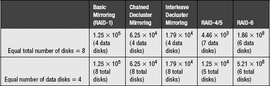
Table 24.2 shows a comparison of the reliability of various mirroring schemes and RAID-5 and RAID-6. A MTTF of 1 million hours is assumed for the disk drives being used. MTTR is assumed to be 1 hour for mirroring and 4 hours for RAID-5/6. These short repair times are based on the assumption that a spare drive is available in the subsystem, so it is not necessary to wait for a replacement drive. The first row is a comparison based on equal total number of disks, with the net number of data disks for each case given in parentheses. The second row is a comparison based on equal number of data disks, with the total number of disks in the array given in parentheses. In both cases, expectedly the double-fault-tolerant RAID-6 has the highest reliability of all array configurations. Among the single-fault-tolerant configurations, basic mirroring has the highest reliability, while RAID-4/5 has the lowest reliability.
No single storage subsystem organization has the best reliability, performance, and cost at the same time. This fact is reflected in the marketplace as subsystems based on mirroring, RAID-5, and RAID-6 are all available with no clear-cut winner. What is the right design choice depends on which one or two of the three characteristics are more important to the user or application.
A quick note about a drive’s MTTF and a subsystem’s MTTDL. An MTTF of 1 million hours may seem like a very long time. Some people may even have the misconception that it means most of the drives will last that long. This is far from the truth. Assuming an exponential failure distribution, i.e., the probability that a drive has already failed at time t is (1 – e–kt), where k is the failure rate, MTTF = 1/k. Then a 1-million-hour MTTF means the drive is failing at a rate of k = 10–6 per hour. By the time MTTF is reached, there is 1 – e–1 = 0.63 probability that the drive would have already failed. For a pool of 1000 drives, statistically 1 drive will have failed in 1000 hours, which is only a little over a month’s time. In five years’ time, about 44 of the drives will have failed. Without fault tolerance to improve reliability, this represents a lot of data loss. The MTTDL numbers listed in Table 24.2 are definitely orders of magnitude better than that of a raw disk. Still, for a subsystem maker that has sold 100,000 eight-disk RAID-5s13 each with an MTTDL of 4.46 × 10³ million hours, in ten years’ time two of those RAIDs will have suffered data loss, even though the owners thought they had purchased a fault-tolerant storage subsystem to provide reliable data storage. This is why subsystems with RAID-6, triplicated or even quadruplicated mirroring, and other more complex schemes for higher fault tolerance are sought after by those businesses for whom data is their lifeline.
The discussion on MTTDL so far is only based on drive failures alone. When other components of a storage subsystem are factored in, such as the electronics, cooling, power supply, cabling, etc., the MTTDL of the entire subsystem will actually be lower. Finally, the MTTDL equations given in this chapter are from highly simplified models and assume disk drive failures are independent, which is an optimistic assumption.
24.3.4 Sparing
It can be seen that in all the above MTTDL equations for various configurations, MTTDL is always inversely proportional to MTTR. This is intuitively obvious, since the longer it takes the subsystem to return to a fault-tolerant state, the bigger the window in which the subsystem is vulnerable to another drive failure. Thus, a key to improving the reliability is to make the repair time as short as possible.
As discussed earlier, repair of a fault-tolerant storage subsystem includes replacing the failed drive and rebuilding its content. Waiting for a repairman to come and swap out the bad drive usually takes hours, if not days. A commonly used strategy for avoiding this long delay is to have one or more spare drives built in the subsystem. As soon as a drive fails, the subsystem can immediately start the repair process by rebuilding onto the spare drive. This essentially makes the drive replacement time zero.
There are two concepts regarding sparing that will be discussed here [Ng 1994c].
Global Sparing
A storage subsystem usually contains multiple RAIDs. While it is probably a simpler design to have a spare drive dedicated to each RAID, a better reliability design and more cost-effective solution is to place all the spare drives together into a common pool that can be shared by all the RAIDs. Without sharing, if one RAID has a failure and consumes its spare drive, it no longer has a spare until a serviceman comes and swaps out the bad drive and puts in a new spare. During this window, that RAID will have a longer repair time should another failure occur. On the other hand, if all spares are shared, then any RAID in the subsystem can go through multiple drive-failure/fast-repair cycles as long as there are still spares available in the pool. Global sparing is more cost-effective because fewer total number of spares will be needed, and the serviceman can defer his visit until a multiple number of spares have been used up instead of every time a spare is consumed.
Distributed Sparing
Traditionally, a spare drive would sit idly in the subsystem until called upon to fulfill its function as a spare. This is a waste of a potential resource. Furthermore, there is always the possibility that the spare will not actually work when it is finally needed, unless the subsystem periodically checks its pulse, i.e., sees if it can do reads and writes.
A better strategy is to turn the “spare” disk into another active disk. This is achieved by off-loading some of the data from the other drives onto this additional drive [Menon et al. 1993]. The spare space is now distributed among all the drives in the array. This is illustrated in Figure 24.9 for a 4 data disk RAID-5. Each parity group has its own spare block, Si, which can be used to hold any of the blocks in its parity group. For example, if Disk 2 fails, then D12 is rebuilt onto S1 in Disk 6, D22 is rebuilt onto S2 in Disk 5, etc., and P4 is rebuilt onto S4 in Disk 3. Note that there is no rebuild for S5. Again, the advantage of distributed sparing is that the total workload to the array is now shared by N + 2 drives instead of N + 1, so total throughput should increase. Reliability should stay about the same. On the one hand, there is now one additional data carrying disk drive whose failure can lead to data loss, so Equation 24.13 for RAID-5 becomes

On the other hand, this is mitigated by the fact that rebuild will be faster because each drive is only(N + 1)/ (N + 2) full, thus the MTTR here is reduced from that of Equation 24.13 by this factor.
24.3.5 RAID Controller
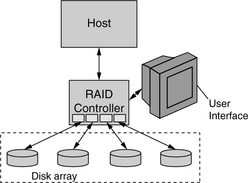
For a group of disks to perform together as a RAID, they must be managed as such. The management function can be performed by software in a host to which the drives of the array are connected directly. This is called a software RAID and is usually found in low-end systems such as personal workstations. More commonly, the RAID functions are handled by a dedicated controller which typically includes some specialized hardware, such as an XOR engine for parity calculations. This type of subsystem is called a hardware RAID. For smaller systems, the controller can be an adapter card that goes on the system bus inside the host. For larger systems, the RAID controller is likely to be an outboard unit. Adapter card RAID solutions are generally fairly basic, support only one or two RAIDs, and are not sharable between different machines. RAID systems with outboard controllers can be shared by multiple clients, so they usually provide more functions, such as zoning/fencing to protect an individual client’s data. They are generally more complex and can support a larger number of RAIDs. Even though a controller failure would not cause data loss, it does make data unavailable, which is not acceptable for 24/7 applications. Therefore, the highest end storage subsystems have dual controllers to provide fail-over capability.
Figure 24.10 shows a simple system configuration for an outboard RAID. The connections between drives and the RAID controller are standard disk interfaces, depending on what types of drives are used. The RAID controller also uses a standard disk interface to connect to the host; however, this does not have to be of the same type as the interface to the drives. For example, the connection between the RAID controller and host may be FC-AL, while drives with an SCSI interface or SATA interface may be used in the array. One of the many functions performed by the RAID controller is to bridge between these two interfaces. The controller provides a user interface that allows the user to configure the drives. Most controllers allow the user to create any combinations of RAID-0, 1, 3, and 5 from the available drives in the array. Many even allow multiple RAIDs to be constructed out of each drive by using different portions of its address space. For example, half of Disk 1 and Disk 2 may form a mirrored pair, and half of Disk 3 and Disk 4 may form a second mirrored pair, with the remaining spaces of Disks 1, 2, 3, and 4 forming a 3 + P RAID-5. Stripe size is usually also selectable by the user; most use the same block size for both parity stripe and data stripe, for simplicity.
Another function performed by the RAID controller is that of caching. The read cache in the controller is typically orders of magnitude larger than the disk drive’s internal cache. This allows full stripes of data to be prefetched from the drives even though only a few sectors may be requested in the current user command. As discussed earlier, the main performance disadvantage of RAID-5/6 is the small block write. Hence, write caching would be very beneficial here. However, traditional caching of writes in DRAM is not acceptable since it is susceptible to power loss. Hence, higher end storage subsystems that provide both reliability and performance use non-volatile storage (NVS), typically by means of battery backup, to implement write caching. Until data is written out to the target drive and the corresponding parity is updated, it is still vulnerable to single fault failure in the NVS. To address this issue, a common solution is to maintain two cached copies of data, one copy in NVS and another copy in regular DRAM. Since different hardware is used for the two copies, a single failure can only wipe out one copy of data.
24.3.6 Advanced RAIDs
Since the introduction of the RAID concept in 1988, others have expanded on this field with additional ideas such as declustered RAID [Mattson & Ng 1992, 1993; Ng & Mattson 1994], cross-hatched disk array [Ng 1994a, 1945], hierarchical RAID [Thomasian 2006], Massive Arrays of Idle Disks (MAID) [Colarelli et al. 2002], etc. In this section, two of these more advanced architectures are discussed.
Declustered RAID
It was pointed out in Section 24.3.2 that in RAID-5 degraded mode, the workload for each surviving drive in the array is roughly doubled (depending on the read-to-write ratio). The situation gets even worse during rebuild mode, when all the drives in the RAID-5 have to participate in the data reconstruction of every read request to the failed drive and at the same time contribute to the rebuild effort of the entire drive. If there are multiple RAID-5s in the subsystem, this means only one is heavily impacted while the other RAIDs are not affected. Using the same logic behind interleaved decluster mirroring (where mirrored data of a drive is evenly spread out to all other drives in the subsystem, instead of being placed all in a single mate drive as in basic mirroring), one can similarly architect a RAID so that its parity groups are evenly distributed among all the drives in the array instead of always using the same set of drives. The resulting array is called declustered RAID.
In a traditional N + P RAID-5, the parity group width is N + 1, and if there are k such RAIDs, the total number of drives T in the subsystem is equal to k × (N + 1). With declustering, there is only one declustered RAID in T drives. There is no fixed relationship between T and N other than (N + 1) < T. Figure 24.11 illustrates a simple example of a declustered RAID-5 with T = 4 total drives and a parity group width of 3. W, X, Y, and Z represent four different parity groups, with each group being 2 + P. Again, Figure 24.11 is only a template for data placement which can be repeated many times. The parity blocks can also be rotated in a similar fashion to RAID-5. The declustering concept can equally be applied to RAID-6.

FIGURE 24.11 A simple example of declustered RAID. There are four total drives. W, X, Y, and Z represent parity groups of width 3.
To generate a declustered array with parity groupings that are uniformly distributed among all the drives, partition each disk into B logical blocks to be used for forming parity groups. In the example of Figure 24.11, B = 3. When forming a parity group, no two logical blocks can be from the same disk, for failure protection reason. Finally, every pair of disks must have exactly L parity groups in common. L = 2 for the example of Figure 24.11. For the reader familiar with the statistical field of design of experiments, it can be seen that the balanced incomplete block design (BIBD) construct can be used to create such declustered arrays.
Hierarchical RAID
While RAID-6 provides fault tolerance beyond a single disk failure, the error coding scheme for the second redundancy can look a little bit complicated. Some have chosen to implement a higher level of fault protection using a different approach, which is to construct a hierarchical RAID using basic levels of RAID such as RAID-1, 3, and 5.
An example is RAID-15 which, in its simplest form, is to construct a RAID-1 on top of two RAID-5s, as shown in Figure 24.12. To the RAID-1 controller on top, each RAID-5 below it appears as a logical disk. The two logical disks are simply mirrored using basic mirroring. For disaster protection, the two RAID-5s can even be located in two different sites, perhaps linked to the RAID-1 controller using optical fiber. Other configurations such as RAID-11, RAID-13, and RAID-51 can be constructed in a similar fashion.

FIGURE 24.12 A Simple RAID-15 configuration. Each RAID-5 appears as a logical disk to the RAID-1 controller.
In the simple configuration of Figure 24.12, the subsystem is fault tolerant to one single logical disk failure, that is, double or more failures in one of the RAID-5s and concurrently a single failure in the other RAID-5. Using exactly the same total number of disks, a more sophisticated RAID-15 would integrate all the RAID-1 and RAID-5 controllers into one supercontroller. This supercontroller will be cognizant of the configuration of all the disk drives in the subsystem. With this intelligent supercontroller, the subsystem can be fault tolerant to more combinations of disk failures. As long as there is only one mirrored pair failure, the subsystem is still working. This is illustrated in Figure 24.13 for a 14-disk RAID-15. Data for all disks except Disk 1 are available. Data for Disk 1 can be reconstructed using RAID-5 parity.

24.4 SAN
As the enterprise computing paradigm evolved during the 1990s from stand-alone mainframes to that of distributed computing with networked servers, the long time I/O architecture of dedicated storage connected directly to a single host machine became inadequate. A new architecture in which storage could be more readily shared among multiple computers was needed. A natural evolution at the time was to have the distributed application servers, each with its own Direct Access Storage (DAS), share data with each other and with clients by sending data over the local area network (LAN) or the wide area network (WAN) that they were attached to. This is illustrated in Figure 24.14. Management of data storage is distributed since it must be handled by the individual servers. This architecture has a few drawbacks. First, in the 1990s, the speed of Ethernet, with which networks were built, was slow in comparison to that of disk drives. Thus, accessing data in a different machine on the LAN suffered from poor performance. Second, sending a large volume of data over the LAN or WAN clogged up the network, slowing other communications between the servers and clients. Third, if a server was down, then the data in its DAS became unavailable to the rest of the system.

FIGURE 24.14 System configuration using DAS. Server A must access the data of Server B over the network.
At about the same time, prodded by customer interest, there was movement afoot for high-end computing to evolve from systems using captive proprietary components of a single manufacturer to an open architecture in which the customer could pick and choose products from multiple vendors based on price, performance, functionality, and reliability instead of on brand name. Furthermore, as demand for data storage space grew exponentially, driven by such new applications as data warehousing and mining, e-mail, and digitization of all information from books to movies, scalability of storage subsystem also became a very important feature for a storage subsystem. Finally, with the cost of storage management becoming a very significant portion of an IT department’s budget, IT professionals were rediscovering the efficiency of centralized data management over distributed management.
In the late 1990s, the concept of storage area network (SAN) was conceived to be the solution that could satisfy all the above requirements. In this architecture, a vast array of open standard storage devices are attached to a dedicated, high-speed, and easily growable backend network. All the data of these devices is accessible to any number of servers that are similarly connected to this network. This is illustrated in Figure 24.15. The resulting decoupling of storage from direct attachment to servers has some important benefits:
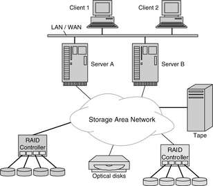
• Placing all data traffic in a separate backend network frees up the LAN/WAN for application traffic only.
• Data availability is improved over that of DAS.
• Maintenance activities can be performed on storage subsystems without having to shut down the servers, as is the case with DAS.
• Non-disk types of storage devices such as tape and optical disks can easily be added and shared.
High-speed Fibre Channel (FC) technology became mature at just about the time that SAN was being proposed. FC switched fabric, discussed earlier in Chapter 20, Section 20.6, seemed to be the perfect instrument for implementing SAN. In fact, one could argue, and perhaps rightfully so, that the idea of SAN was really the product of the availability of FC technology. By leveraging the topological flexibility afforded by FC switched fabric’s connectivity, SAN can be configured in many shapes and forms. SAN also inherits the multi-gigabit speed of FC, which additionally allows remote placement of storage subsystems a long distance away from servers when optical cables are used.
With SAN technology, all the storage space of a subsystem appears to the user as logical volumes. Thus, data is accessed at the block level, with file systems in the servers managing such blocks.
24.5 NAS
The flexibility of SAN comes at a cost. For smaller systems the price of acquiring an FC switched fabric may be too high an entry fee to pay. Vendors in the storage industry offer an alternative approach for off-loading data traffic and file service from an application server with captive DAS, while at the same time providing an easier path to scalability with a subsystem that is relatively simple to deploy. Such products are called network attached storage (NAS).
NAS is a specialized device, composed of storage, a processor, and an operating system, dedicated to function solely as a file server. While it can certainly be implemented using a general-purpose machine with a general-purpose, full-function operating system such as Unix or Windows, it is cheaper and simpler to use stripped down hardware and software to perform its one specific function. Such a slimmed down system is sometimes referred to as a thin server. The major pieces of software required by NAS are a file system manager, storage management software, network interface software, and device drivers for talking to the disk drives.
As its name implies, NAS is connected to a working group’s LAN or WAN, and its data is accessed by clients and application servers over the network. This is illustrated in Figure 24.16. TCP/IP is typically the networking protocol used for communication. Some NAS products support Dynamic Host Configuration Protocol (DHCP) to provide a plug-and-play capability. When connected to the network, they discover their own IP addresses and broadcast their availability without requiring any user intervention.

Unlike SAN, where storage data is accessed in blocks, in NAS the user does file accesses. Two main network file access protocols are most commonly used. They are the Network File System (NFS) and the Common Internet File System (CIFS). NFS was introduced by Sun Microsystems in 1985 and is the de facto standard for Unix types of systems. CIFS is based on the Server Message Block (SMB) protocol developed by Microsoft, also around mid-1980s, and is the standard for Windows-based systems. Due to the fundamental differences between these two protocols, most NAS subsystems are used exclusively by either all Unix or all Windows machines in a network, but not both at the same time.
Since NAS uses the working group’s network for data transfer, it is not an ideal solution for regularly transferring a large volume of data, as that would create too much traffic on that network. SAN is more suitable for that purpose. On the other hand, low entry cost and ease of deployment make NAS an attractive solution for file sharing purposes within a small working group. In fact, some IT system builders may find SAN and NAS technologies complementary and able co-exist within the same system.
24.6 iSCSI
SAN allows users to maintain their own files and do block access to the storage of SAN, but requires the addition of an FC switched fabric. NAS does not require any additional networking equipment, but users have to access data at the file level (not implying that it is good or bad here). The storage industry came up with a third choice for users which is a combination of these two options. In this third option, the storage subsystem is attached to the work group’s network, as in NAS, but data access by the user is at the block level, as in SAN. This technology is called iSCSI, for Internet SCSI. It was developed by the Internet Engineering Task Force (IETF) and was ratified as an official standard in February 2003.
In iSCSI, SCSI command-level protocols are encapsulated at the SCSI source into IP packets. These packets are sent as regular TCP/IP communication over the network to the SCSI target. At the target end, which is a dedicated special iSCSI storage server, the packets are unwrapped to retrieve the original SCSI message, which can be either command or data. The iSCSI controller then forwards the SCSI information to a standard SCSI device in the normal fashion. This is illustrated in Figure 24.17.

With the availability of Gigabit and 10-Gbit Ethernets, the raw data rate of iSCSI becomes competitive to that of FC. Efficient network driver code can keep the overhead of using TCP/IP to an acceptable level. Hardware assist such as the TCP Offload Engine (TOE) can also reduce overhead.
1Actually, synchronizing the rotation of the disks would not necessarily help either, since the first stripe unit of a file in each of the drives may not be the same stripe unit in all the drives. As File f in Figure 24.1 illustrates, f1 and f2 are the second stripe unit in Disks 2 and 3, but f3 is the third stripe unit in Disk 1.
2Track skew is ignored in this simple analysis.
3Later, in Section 24.3.2, there is an opposing argument for using a smaller stripe size.
4The queueing delay is inversely proportional to (1 – utilization). Thus, a drive with 90% utilization will have 5× the queueing delay of a drive with 50% utilization.
5For very critical data, more than two copies may be used.
6A duplicate copy of certain critical data, such as boot record and file system tables, may also be maintained in the same drive to guard against non-recoverable errors. This is independent of mirroring.
7The word “inexpensive” was later replaced by “independent” by most practitioners and the industry.
8The choice of using the word “level” is somewhat unfortunate, as it seems to imply some sort of ranking, when there actually is none.
9A (n,k) code means the code word is n bits wide and contains k information bits.
10In practice, byte-level striping is more likely to be used as it is more convenient to deal with, but the concept and the net effect are still the same.
11RAID-5 is oftentimes described as an N + P disk array, with N being the equivalent number of data disks and P being the equivalent of one parity disk. Thus, a 6-disk RAID-5 is a 5 + P array.
12RAID-6 is oftentimes described as an N + P + Q array, with N being the equivalent number of data disks, P being the equivalent of one parity disk, and Q being the equivalent of a second redundant disk. Thus, a 6-disk RAID-6 is a 4 + P + Q array.
13A medium-size installation typically has hundreds of disk drives.