
Performance Issues and Design Trade-Offs
In this chapter, we will examine certain aspects of disk drive performance in more detail. Some of the topics covered earlier are revisited here again, with the purpose of discussing some of their performance issues and analyzing their related design trade-offs. Chapter 16, Section 16.4, “Disk Performance Overview” has some introductory discussion of disk performance. This is a good time to review that section before continuing with this chapter.
19.1 Anatomy of an I/O
The one underlying thing that determines both response time and throughput of a disk drive is the I/O completion time [Schwaderer & Wilson, 1996, Ng 1998, Ruemmler & Wilkes 1994]. The time required by a disk drive to execute and complete a user request consists of four major components: command overhead, seek time, rotational latency, and data transfer time, as diagrammed in Figure 19.1.
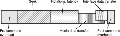
1. Command overhead This is the time it takes for the disk drive’s microprocessor and electronics to process and handle an I/O request. This is usually not a simple fixed number, but rather depends on the type of drive interface (ATA, SCSI, or FC), whether the command is a read or a write, whether the command can be satisfied from the drive’s cache if it is a read, and whether write cache can be used if it is a write. Most of the overhead occurs at the beginning of an I/O, when the drive controller needs to interpret the command and allocate the necessary resources to service the command, and then again at the end of the I/O to signal completion back to the host and also to clean up. Certain processing by the disk drive controller may be overlapped with other disk activities, such as doing command sorting while the drive is seeking. As such, they are not counted as overhead here; only non-overlapped overhead is counted. Like all other disk drive parameters, command overhead has been steadily declining over the years due to faster embedded controller chips and more functions, such as cache lookup, being handled by hardware.
2. Seek time This is the time to move the read/write head from its current cylinder to the target cylinder of the next command. Because it is mechanical time, it is one of the largest components of an I/O and naturally has been receiving a lot of attention. Seek time has been decreasing ever since the early IBM RAMAC days. Much of the improvement comes from smaller and lighter drive components, especially shrinking disk diameter, as shown in Chapter 16, Figure 16.3, since it means the arm has less distance to travel. Smaller disk diameter also means the actuator and arm can be lighter and therefore easier to move. Seek time is composed of two sub-components, viz., the travel, or move, time and the settle time—the time after arriving at the target track to when correct track identification is confirmed and the head is ready to do data transfer. As seek distance decreases, settle time becomes a relatively more important component. Typical average seek time for today’s server drives is about 4 ms, while for desktop drives it is about 8 ms. Mobile drives for power conservation reasons are typically slower. Seek time will be discussed further in Section 19.2.3.
3. Rotational latency Once the head has arrived at the target cylinder and settled, rotational latency is the time it takes for the disk rotation to bring the start of the target sector to the head. Since magnetic disk drive’s rotational speed is constant, the average rotational latency is simply one-half the time it takes the disk to do one complete revolution. Therefore, it is inversely proportional to rotational speed. Here again, because it is also mechanical time, it is another one of the largest components of an I/O. The drive’s rpm, for some reason, does not make gradual evolutionary improvements like most other disk drive parameters, but goes up in several discrete steps. This step-wise progress of rpm and its associated average latency are plotted in Figure 19.2. Just because a new higher rpm is being introduced does not mean all disk drives being manufactured will immediately be using the higher rpm. Usually, higher rpm is first introduced in the high-end server drives. It takes a few years for the majority of server drives to adopt the new speed, then it takes another few more years before it becomes commonplace among desktop drives, and then it takes yet another few more years for it to be introduced in mobile drives. Take 7200 rpm, for example. It was first introduced in server drives back in 1994, but it was not until the late 1990s before it appeared in desktop drives. The first 7200 rpm mobile drive was not available until 2003, almost ten years after the first 7200 rpm drive was introduced. Today’s high-end server drives run at 15K rpm, with 10K rpm being the most common, while desktop drives are mostly 7200 rpm.

FIGURE 19.2 Year of first introduction of (a) rpm and (b) associated rotational latency. Note that just because a higher rpm is introduced in one drive model, it does not mean all other drive models will also use that new rpm.
4. Data transfer time Data transfer time depends on data rate and transfer size. The average transfer size depends on the host operating system and the application. While there may be some gradual increase in average transfer size over time, with some video applications transferring 256 KB or more per I/O, a more modest 4-KB transfer size is still fairly common today.
There are two different data rates associated with a disk drive: the media data rate and the interface data rate. The media data rate is how fast data can be transferred to and from the magnetic recording media. It has been increasing continuously over the years simply as a consequence of increasing recording bit density and rotational speed. For instance, today a typical server drive rotating at 10K rpm with 900 sectors (512 data bytes each) per track will have a user media data rate of 75 MB/s. Sustained media data rate was discussed in Chapter 18, Section 18.8. Interface data rate, on the other hand, is how fast data can be transferred between the disk drive and the host over the interface. The latest ATA-7 standard supports interface speeds up to 133 MB/s. For SCSI, the data rate for the latest Ultra 320 standard is 320 MB/s for a 16-bit-wide bus. SATA (serial ATA) and SAS (Serial Attached SCSI), both of which share compatible cabling and connectors, support interface speeds up to 300 MB/s, with future plans for 600 MB/s. FC is currently at 200 MB/s and working on 400 MB/s. All these interfaces are substantially faster than the media data rate.
For reads, most of the interface data transfer can be overlapped with the media data transfer, except for the very last block, since every sector of data must be all in the drive buffer for error checking and possible ECC correction before it can be sent to the host. For interfaces where the drive disconnects from the bus during seeks, ideally it should time the reconnection of the bus such that interface data transfer of the next to last sector will be finished just in time when the media transfer of the last sector is completed and is ready to be sent back to the host. For writes, all of the interface data transfer from the host can be overlapped with the seek and latency time, spilling over to overlap with the media transfer if necessary.
19.1.1 Adding It All Up
These I/O time components are put into perspective for the two major types of I/O requests.
Random Access
Consider a hypothetical 10K rpm disk drive with an average media transfer rate of 50 MB/s and an interface of 100 MB/s. Assume an average seek time of 4.5 ms and overhead of 0.3 ms. The time for one revolution is 6 ms, so the average rotational latency is 3 ms. The media transfer time for 4 KB is 0.08 ms, and the interface transfer time for the last sector is 0.005 ms. Therefore, the average time to do a random read of a 4-KB block with this disk drive is
For many applications and systems, I/Os are not completely random. Rather, they are often confined to some small address range of the disk drive during any given short window of time. This phenomenon or behavioral pattern is called locality of access. The net effect is that the actual seek time is much smaller than the random average, often roughly one-third of the average. Hence, in this local access environment, the average time to read the same 4-KB block becomes
Figure 19.3 graphically illustrates the relative contributions of the four major time components of an I/O to the overall disk I/O time, for both random access and local access. It shows that for local access, which is likely to be the dominant environment for single user machines or small systems, rotational latency accounts for the greatest share of I/O time. For disk drives used in very large servers receiving I/O requests from many different users, a more or less random request pattern is probably more likely. For such random I/Os, seek time is the biggest component. Note that for 4-KB accesses, which is a typical average in many operating systems and applications, the data transfer time is rather insignificant compared to the mechanical times.

Sequential Access
Understanding the performance of a drive in servicing a random access is important because this type of I/O exacts the greatest demand on a drive’s available resources and is also most noticeable to the user due to its long service time. The overall performance of a drive for most classes of workloads is generally gated by how fast it can handle random accesses. Yet, on the flip side, sequential access is an important class of I/O for exactly the opposite reasons. It can potentially be serviced by the drive using only the least amount of resources and be completed with a very fast response time.
A sequential access is a command in which the starting address is contiguous with the ending address of the previous command, and the access types (read or write) of both commands are the same. If handled properly, such a command can be serviced without requiring any seek or rotational latency. Using the parameters of the hypothetical drive above, the service time for a sequential 4-KB read is only
Compared to 7.885 ms for a random access, it is an order of magnitude of difference. Thus, a good strategy, both at a system level and at the drive level, is to make the I/O requests as seen by the drive to have as high a fraction of sequential accesses as possible. Naturally, it is important that a disk drive handles sequential I/Os properly so that it does not miss out on the good performance opportunity afforded by this type of access.
In addition to strictly sequential I/O, there are some other types of commonplace accesses that also have the potential of being serviced by the drive with very short service times if handled properly,
• Near sequential. Two commands that are otherwise sequential separated by a few (no precise definition) other commands in terms of arrival time at the drive.
• Skip sequential. Two back-to-back commands where the starting address of the second command is a small (no precise definition) number of sectors away (in the positive direction) from the ending address of the previous command, and the access types (read or write) of both commands are the same. Note that this is similar, but not identical, to stride access, a behavior observed and exploited in processor design wherein the application walks sequentially through data with a non-unit offset between accesses (e.g., addresses 1, 4, 7, 10, 13, …).
• Near and skip sequential. Combination of both near sequential and skip sequential.
The ability of a drive to take advantage of the close spatial and temporal proximity of these types of I/Os to reduce service time is an important facet in creating a drive with good performance.
19.2 Some Basic Principles
Disk drive performance is improved when I/O completion time is reduced. Hence, anything that directly shortens one or more of the four major components of an I/O will obviously improve performance. Disk drive makers are always on a quest to shorten the seek time by designing faster actuators to cut down the move time and adding more servo wedges per revolution to decrease the settle time. As discussed earlier, rotational speed has been increasing over the years mainly to cut down rotational latency time, but as a side benefit it also results in increasing the media data transfer rate and, hence, reducing data transfer time. The performance impact of such direct performance improvement design actions is self-evident and needs no additional discussion in this chapter. Other more elaborate techniques and schemes for reducing seek time and rotational latency time are discussed in Chapter 21.
In this section, several fundamental guiding principles governing disk drive performance which go somewhat beyond the obvious are laid down. The performance impact of any design trade-off can then be interpreted using one or more of these principles [Ng 1998].
19.2.1 Effect of User Track Capacity
The capacity for user data on a track is completely specified by the number of sectors on that track, SPT as previously defined. Some of the things that affect this number are:
Many factors affect the formatting efficiency. Refer back to Chapter 18 for a detailed discussion.
Increasing the user track capacity has several effects on a drive’s performance, which are discussed in the following.
Media Data Rate
As indicated in Chapter 18, Equations 18.13 and 18.14, user data rates are directly proportional to the SPT number. As a higher data rate reduces data transfer time, this effect is obviously good for performance. While for a 4-KB random access this effect is negligible, as discussed above, faster media data rate is important for applications that do large sequential accesses. Unlike random access, an I/O in a properly handled stream of sequential accesses does not require any seek or rotational latency. Furthermore, because the interface data rate is typically faster than the media data transfer rate, the media data rate is the gating factor in determining the performance of large sequential accesses. Proper handling of the drive’s cache should allow most, if not all, of the overheads to be overlapped with the media data transfer, as discussed in Chapter 22 on caching.
Number of Track/Cylinder Switches
Whenever the end of a track is reached, some amount of finite time is required to either switch to the next head in a cylinder (head switch) or move the actuator to the next track or cylinder (cylinder switch), as discussed in Chapter 18. The time to do the switch is hard-coded in the disk drive geometry in the form of track skew or cylinder skew and is typically of the order of 1 or 2 ms. This switch time adds to the total I/O time, as part of the data transfer time, if the requested piece of data spans multiple tracks or happens to cross a track boundary.
For example, consider the same drive parameters as in Section 19.1.1, and assume a track switch time of 1.5 ms. The same 4-KB local access that normally takes 4.885 ms to complete will now take 6.385 ms, an increase of 30%, if that data block happens to cross a track boundary.
For a request size of K sectors, the probability that this request will cross a track boundary is
For a drive using the serpentine formatting, in addition to the actual media transfer time, the average data transfer time for a request of K sectors needs to be increased by an average switch time TS,
where TCS is the cylinder switch time. A drive with N heads and using the cylinder mode formatting will have an average switch time of
where THS is the head switch time. Since pcross is inversely proportional to SPT, increasing the track capacity will reduce the probability of a block crossing a track boundary and, hence, the average added switch time. This is, of course, good for performance.
Constraint on rpm
While increasing the media data rate and reducing the average add-on switch time are good for improving performance, increasing the track capacity too much may run into the possibility of pushing the data rate beyond what the drive’s data channel can handle. This limitation can be due to either technology or cost consideration. While today’s disk drive read/write channel electronics can comfortably handle the media data rate encountered in any drive, things can look different if there is a new technology breakthrough that suddenly sends linear density and data rate soaring. For a given radius, bpi and rpm are the two main factors that determine data rate. Hence, when bumped up against this limit, the disk drive designer is faced with a dilemma: forfeit some of the increase in bpi and thus the drive would not gain as much capacity as it otherwise would, or reduce the rotational speed. Neither is desirable. Even if channel technology can keep up with the bpi increase, putting a limitation on increasing rpm is an impediment to improving performance.
This brings up a third design choice, and that is to decrease the diameter of the disk. Going with a smaller disk diameter has the additional advantage of making it mechanically easier to spin the disk faster. Indeed, these are some of the reasons for the downward trend in disk diameter, as shown in Chapter 16, Figure 16.3. The trade-off here is, of course, reduced drive capacity when disk diameter is smaller. As a matter of fact, 3.5” form factor, 15K rpm server drives typically use 70-mm diameter disks internally, even though 95-mm disks are used in 7200 rpm desktop drives with the same form factor.
19.2.2 Effect of Cylinder Capacity
An increase in the capacity of a cylinder can be brought about in one of two ways:
• Increase in track capacity—this, in turn, can be due to several different factors, as discussed in the previous section
• Increase in the number of heads and recording surfaces in a cylinder
In many systems, especially single-user personal computers, only one or a few applications are active at a time. In such an environment, typically just a small fraction of the disk drive’s data is being accessed during any window of time. When operating within a narrow range of data, having more data sectors in a cylinder has two effects:
1. The seek distance is reduced For example, assume bpi is increased by 33%, resulting in the size of each cylinder increasing by the same percentage. Then, a fixed amount of data would now occupy only 100/133 = 75% as many cylinders as before. As a result, seek distance within this range of data would, on average, be reduced by 25%. Shorter seek distance means shorter seek time.
2. The number of seeks is reduced When dealing only with a small amount of data, having a cylinder with larger capacity increases the likelihood that the next piece of data required by the user will be found in the current cylinder, thus avoiding a seek completely. For instance, assume a user is working on a file which is 64 MB in size. For a hypothetical drive with 4 tracks per cylinder and 300 KB per track, the probability that two different sectors from that file are located in the same cylinder is
Switch to another hypothetical drive with 8 tracks per cylinder and 500 KB per track, the probability increases to
These two effects of having a more capacious cylinder result in either shortening or eliminating seek time, thereby improving performance. This is illustrated by using an event-driven simulator which tracks the total number of seeks and total seek time. A hypothetical disk drive with 900 sectors per track is simulated, first with 1 track per cylinder as the base and then with 2, 4, and 8 tracks per cylinder. This is one way to compare the effect of cylinders whose capacities are 2×, 4×, and 8× that of the base case. A trace of over 10 PC applications with about 15K reads and about twice as many writes is used as the input. Figure 19.4 shows (a) the total number of seeks and (b) the total seek times for all the reads; the effect on writes is very similar and not shown here. The beneficial effect of having a larger cylinder is clearly illustrated by this simulation result.
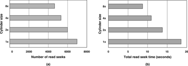
FIGURE 19.4 Simulation showing the effect of cylinder size on seek: (a) total number of seeks and (b) total seek time.
Keep in mind that the concept of a cylinder applies only if the disk drive uses the cylinder mode formatting. While the above discussion has no meaning for a drive using the straight serpentine formatting, however, the reduced seek distance effect does apply to some extent to drives using the banded serpentine formatting. In fact, the narrower the band is, the more the above applies—one can think of cylinder mode as banded serpentine where the width of a band is one track.
19.2.3 Effect of Track Density
Unlike the previous two disk drive characteristics which can be affected by other characteristics, track density can only be influenced by one thing, namely tpi (tracks per inch). The main impact that tpi has on performance is in its seek time. Seek time consists of two components: (1) a travel time for the actuator to move from its current radial position to the new target radial position and (2) a settle time for centering the head over the target track and staying centered so that it is ready to do data access:
seek time = travel time + settle time (EQ 19.9)
Travel Time
The travel time is a function of how far the head needs to move. This distance, in turn, is a function of how many cylinders the head needs to traverse and the disk’s tpi, as given by this relationship:
seek distance = number of cylinders of seek / tpi (EQ 19.10)
In a simplistic case, to complete the travel in the shortest time, the actuator would accelerate at its maximum acceleration until half the seek distance is covered and then decelerate at an equal rate (by reversing the current in the VCM so that a torque in the opposite direction is applied). This bang-bang seek model is illustrated in Figure 19.5(a), which plots both the acceleration and the velocity as a function of time. For such a model, the seek time is given by
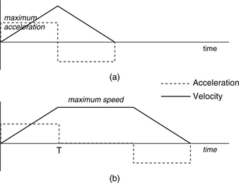
from elementary physics. This model is only approximate because today all drives use rotary actuators, and so the seek “distance” should really be measured by the angle that the actuator needs to rotate. Such an angle for any given number of tracks is dependent on the radial positions of those tracks on the disk. However, the above linear approximation model is adequate for our discussion here.
The bang-bang seek is applicable up to a certain seek distance. Beyond that, it may be necessary to limit the actuator speed not to exceed some maximum limit. For one reason, if the head is travelling too fast, then it could be crossing too many tracks in between servo wedges, meaning it would be flying blind for too long without getting feedback on its current location and progress. Another consideration may be that the head stack must not hit the crashstop at excessive speed should power be lost in the middle of a seek. Power consumption may be yet another limiting consideration, especially for portable computers or devices. Hence, for longer seeks, acceleration may be turned off once the maximum speed has been reached, and the actuator coasts until it is time to decelerate. This is illustrated in Figure 19.5(b). For this model, the travel time is given by
travel time = T + seek distance / (acceleration × T) (EQ 19.12)
where T is the time required to reach maximum speed, which is maximum speed divided by acceleration. The difference in the travel time profile between a bang-bang seek (no speed limit) and one which coasts after reaching a maximum speed limit is illustrated in the example shown in Figure 19.6. In this example, the seek distance is expressed as a fraction of the maximum (full stroke) seek, and the travel time is normalized to an acceleration unit of 1. Thus, from Equation 19.11, the full stroke or maximum seek time is 2 units. T is set to 0.5 in this example, which occurs at a seek distance of 12.5% of full stroke. Any seek distance greater than 25% of full stroke will require part of its travel limited to coasting at the maximum allowed speed. In this case, the coasting method is 25% slower than the aggressive bang-bang method in the worse case, as illustrated in Figure 19.6.
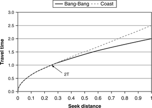
FIGURE 19.6 Example of travel time profiles for two strategies. Normalized to acceleration of 1 unit. Example is for T = 0.5 unit.
Because seek distance is inversely proportional to tpi, as stated in Equation 19.10, regardless of whether the seek is for a short distance or for a longer distance, both Equations 19.11 and 19.12 show that travel time will be reduced if tpi is increased. Hence, the travel time component of seek time is improved with higher track density. This statement is true only for seeking between two given logical blocks. The tpi would not have any effect on the travel time of a totally random seek.
Today, many drives that are used for consumer electronics have a “quiet seek” mode. When used in this mode, the drive does not try to achieve fastest seek performance, but rather accelerates and decelerates the actuator at a lower rate so as to cut down on the acoustic noise generated. Since slower acceleration is achieved by applying less current to the VCM, power consumption is also reduced as an added side benefit, and less heat is also generated. However, performance is traded off in return for such benefits.
Settle Time
While travel time is relatively simple, settle time is more complex and depends on many factors. To achieve a faster total seek time, the servo system is designed to be slightly underdamped. Thus, the actuator will overshoot the destination track by a small amount and wobble back and forth a few times before the ringing dies out. The alternative to overshooting is to gracefully approach the destination track more slowly and carefully, but that would increase the travel time, resulting in a longer total seek time.
Settle time is often defined as the time from when the head is within half a track from the destination track’s center line to when the head is ready to do data transfer. Some drives define it as ready to read if it is within about 10% of the track center line (relative to the track width) and can successfully read several correct SIDs in a row. Because it is a much bigger problem if a write is mishandled (off-center or, worse, wrong track) than a read, the write settling condition is more stringent than that for read settling. Hence, it is quite typical for write settling time to be about 0.5 ms longer than read settling time. This is the reason for write seek time being spec’ed higher than read seek time.
When every other factor is the same, it is intuitive that tracks that are narrower and closer together would require a longer settle time. Indeed, a simplistic first-order approximation model of the settling time is
settle time = C × ln(D × tpi) (EQ 19.13)
where C and D are some constants specific to the disk drive. This equation indicates that settle time goes up with tpi logarithmically.
Disk drive designers have been combatting this undesirable effect of tpi increase with different techniques. A standard technique is to increase the bandwidth of the servo system. Newer techniques include more clever algorithms for determining that the drive is ready to do data transfer earlier. Such methods have been able to keep the settle time more or less constant despite rising tpi. However, it is becoming harder and harder to maintain this status quo.
To summarize, tpi has two opposing effects on the seek time of an I/O. Higher tpi shortens the physical seek distance and hence can shorten the travel time. On the other hand, higher tpi may increase the settle time. Thus, whether increasing tpi is good for performance depends on which of these two opposing effects is more dominant. In many applications, the user accesses only a small portion of the disk during any window of time. In such cases, seek distance is short, and the settle time dominates, making increasing tpi bad for performance.
19.2.4 Effect of Number of Heads
It is common practice for drive manufacturers to take advantage of an increase in recording density to reduce the cost of a disk drive by achieving a given capacity using fewer disk platters and heads. This approach has been applied for many years to deliver a lower cost, but equal capacity version of an existing product. For instance, say, an older recording technology allows 80 GB of data to be stored on one disk platter. A 400-GB drive would require five platters. If the next generation of recording density is increased by 67%, then only three platters would be required to provide the same 400-GB capacity. Saving two platters and four heads represents a very substantial reduction in cost.
The effect that the number of heads in a disk drive has on performance depends on whether the drive is using the cylinder mode formatting or the serpentine formatting. In cylinder mode formatting there are two effects:
Data Rate
This effect is a little subtle and kind of minor. Here, we consider the effect of the number of heads in a drive when everything else is equal. This would be the case of comparing the performances of two drives having different capacities within the same family. Referring back to Chapter 18, Equation 18.14, on sustained data rate, let’s assume the head switch time THS to be 10% of the time of one disk revolution, and let K be the ratio of the cylinder switch time TCS to the head switch time THS. Then, Chapter 18, Equation 18.14, can be restated as
If the sustained data rate for N heads is normalized to that of a drive with a single head, the ratio is
Since cylinder switch time is typically higher than head switch time, i.e., K > 1, it can be seen from Equation 19.15 that the sustained data rate is higher with a greater number of heads. This simple relationship is illustrated in Figure 19.7, which shows the sustained data rate, normalized to that for N = 1, for N from 1 to 10, and for values of K = 1, 2, and 3. It can be seen that when K = 1, i.e., cylinder switch time is the same as the head switch time, the number of heads has no effect on the sustained data rate. When K > 1, the sustained data rate goes up with the number of heads, and the effect is greater with a larger difference between cylinder switch and head switch times. Again, this comparison is for when everything else is equal. If the number of heads is reduced as a result of increased bpi, then the increase in data rate due to a greater number of sectors per track will more than offset the minor effect of head and cylinder switches.

Cylinder Size
An increase in areal density is a result of increases in both bpi and tpi. Hence, if the number of heads is reduced as a result of taking advantage of a higher recording density to achieve constant drive capacity, then the total number of sectors in a cylinder actually decreases. In fact, the capacity of a cylinder needs to be decreased by the same factor that tpi is increased in order for the drive net capacity to stay constant. Since bpi also goes up, a decrease in the number of sectors in a cylinder would have to come from having fewer heads.
One of the benefits of a bigger cylinder is that the number of seeks is reduced, as discussed earlier in Section 19.2.2. A smaller cylinder, then, would have just the opposite effect, increasing the number of seeks and therefore hurting performance.
However, there is no change in the average physical seek distance in this case. This is because even though the seek distance in the number of cylinders is increased, the track density is also increased by the same factor. Consider an example where the original drive has 2400 sectors per cylinder—3 heads with 800 sectors per track. If tpi is increased by 33% and bpi is increased by 12.5%, then a new drive with the same capacity would only have 1800 sectors per cylinder—2 heads with 900 sectors per track. In the space of 3 cylinders of the original drive, there are 3% 2400 = 72,000 sectors. In that same amount of space, due to a 33% increase in tpi, the new drive can hold 4 cylinders, for a total capacity of 4%1800 = 72,000 sectors, the same as before. Hence, seeking from one sector to another sector will require crossing 33% more cylinders in the new drive, but the physical distance remains the same. While the physical seek distance may remain the same, the effect of higher tpi on the settle time was discussed earlier in Section 19.2.3.
Serpentine Formatting
For drives using the serpentine formatting, since a track switch taking TCS is always involved at the end of a track, the number of heads in the drive has no effect on its sustained data rate. Instead, the number of heads affects performance through different dynamics involving whether the number of heads is even or odd.
When the number of heads is even, as was illustrated in Figure 18.4(b) in Chapter 18, the head stack ends up at the end of a band in the same radial position as when it started. Hence, a long seek is required to position the head stack to the next band. This is a break in the physical sequential nature of things. While this would not affect performance of a workload that is random in nature, it would most certainly affect the performance of sequential accesses around band boundaries.
On the other hand, when the number of heads is odd, the head stack ends up at the end of each band in the opposite radial position as when it started. Thus, it can move to the beginning of the next band without incurring any long seek. Figure 19.8 shows two ways of laying out the data for an odd number of heads, one requires switching heads while the other does not require switching heads. Not having to switch heads will perform a little faster since one track seek with the same head can be carried out without the uncertainty associated with head switch.

19.3 BPI vs. TPI
An increase in areal density, which is happening at an amazing rate for so many years as discussed in Chapter 16, comes from increases in both bpi and tpi. With the understandings gained in the previous sections, we can now discuss, if given a choice, whether it is more desirable to increase bpi more or tpi more.
An increase in bpi leads directly to increasing track capacity, which is good for performance. An increase in track capacity can, in turn, lead to increasing cylinder capacity, which is also good for performance. Hence, an increase in bpi, as long as it is done within the capability of what the state-of-the-art read/write channel can handle, is a good thing.
An increase in tpi, on the other hand, can eventually lead to a higher settle time. Couple that with the possibility that cylinder capacity may be decreased to take advantage of an increase in tpi as a means to lower cost, then increasing tpi is not likely to be beneficial to performance.
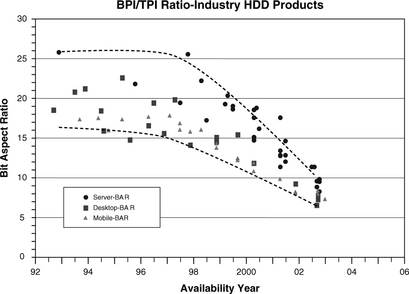
Therefore, if there is a choice, it is more desirable to grow areal density by increasing bpi rather than tpi. Unfortunately, the industry trend seems to be doing the opposite. Figure 19.9 shows the historical trend of the ratio of bpi to tpi (sometimes called the bit aspect ratio). In the early 1990s, this ratio hovered around 20. Today, this ratio is less than 10. This means that tpi is increasing at a faster rate than bpi. Indeed, in recent years the annual compound growth rate (CGR) for bpi has been about 30%, while the CGR for tpi has been about 50%.
19.4 Effect of Drive Capacity
For a random I/O, the capacity of a drive has no direct effect on its performance. However, because of the way some file systems manage and use the space of a disk drive, a drive’s capacity can itself have an effect on users’ or applications’ performance. File systems assign disk space to a user’s file in allocation units, basically fixed-size chunks of sectors. These allocation units must be kept track of in tables—which units are free and which units are assigned to what files.
There is a great variety of file systems, and they have different architectures and data structures. Some use more elaborate schemes and table structures for faster searches of free space and file locations. Some file systems keep track of the allocation status of units using a bit map—one bit for each allocation unit. Windows NTFS file system and the file systems for various flavors of Unix/Linux are examples of this type of file system. Invariably, pointers are needed to point to the allocation units that have been assigned to each file. One of the simplest forms of allocation structure is a table in which each entry in the table corresponds to one allocation unit. With such an architecture, the table size can get unwieldy if small allocation unit size is used for a disk drive with large capacity, as there will be a huge number of allocation units. An example of this type of file system is Windows FAT (File Allocation Table) file system.1 Since Windows operating systems and FAT file systems are so ubiquitous, it is worth spending some time here to discuss this particular type of file system.
For the allocation table type of file systems, in order to keep the table for managing allocation units reasonably small, one approach is to limit the number of such units for a given disk drive by increasing the size of an allocation unit as disk capacity increases. Thus, when the capacity of a disk is doubled, one could either keep the allocation unit size the same and double the size and number of entries of the file system’s table, or one could double the size of each allocation unit and retain the original size of the file table.
As an example, the FAT32 file system for Windows uses a 4-byte file allocation table entry for each allocation unit, which is called a cluster. Hence, each 512-byte sector of the file allocation table can hold the entries for 128 clusters. If the cluster size is 1 KB, then for a 256-GB drive2 a FAT table with 256M entries would be needed, taking up 1 GB of storage space or 2 million sectors. If the cluster size is increased to 64 KB each, then the FAT table size can be reduced by a factor of 64, down to only 16 MB.
The choice of the allocation unit size affects both how efficiently the disk drive’s storage space is used and the performance of user’s application I/Os.
19.4.1 Space Usage Efficiency
The previous discussion indicates that a larger allocation unit size results in a smaller file system allocation table and, therefore, saves space for this overhead. However, this does not necessarily mean that a larger allocation unit size translates to better space usage efficiency. This is because file space allotted to a file is allocated in multiples of allocation units. Space not used in the last allocation unit of each file is wasted, as it can not be used by anyone else. This is the internal fragmentation issue, previously discussed in Chapter 18. This wastage is sometimes referred to as slack by some.
If file sizes are completely random and equally distributed, then on average each file would waste the space of half an allocation unit. So, for example, if there are 20,000 files on the disk drive and the allocation unit size is 64 KB, 20,000 × 32 KB = 640 MB of storage space is wasted due to internal fragmentation. On the other hand, if 1-KB allocation units are used instead, then the amount of wasted space is reduced to only 10 MB. Going back to the FAT32 example above for a 256-GB drive, a 1-KB cluster size requires 1 GB of file allocation table space, but wastes only 10 MB of storage space with 20,000 user files, while a 64-KB cluster size requires only 16 MB of table space, but wastes 640 MB of storage space for the same number of files.
In reality, things can be even worse for a larger allocation unit size, such as 64 KB. This is because many files are small, and hence, more than half of an allocation unit’s space is going to be wasted. For instance, if 80% of the user’s 20,000 files have an average size of 4 KB, then those 16,000 files alone would be wasting 16,000× (64–4) KB = 960 MB of storage space, plus the remaining 20% would be wasting 4000 × 32 KB = 128 MB of storage space, for a total of 1.088 GB.
Naturally, the correct choice of allocation unit size, from a space efficiency point of view, depends on the dominant file size of the user or application. If the typical file size is large, such as files for videos or pictures, a larger allocation unit size is appropriate. If the typical files are small, then allocation units with a smaller granularity are better. The correct choice for a drive (or a volume) with storage capacity C is an allocation unit size U that minimizes:
FS overhead = allocation table size + expected wasted space (EQ 19.16)
where
allocation table size = allocation table entry size × C / U (EQ 19.17)
and
expected wasted space = expected number of files × U / 2 (EQ 19.18)
19.4.2 Performance Implication
One clear advantage of a larger allocation unit size, and, therefore, a smaller allocation table, is that with a smaller allocation table there is a higher probability that the needed allocation table entry to process a user’s access request will be found in cache, either the disk drive’s internal cache or the cache in the host system, and an entry that can be looked up in a cache is much faster than one requiring a disk access. This comes about in two different ways:
• A very large table would not all fit in the cache. On the other hand, the smaller the table is, the higher percentage of its content would be in the cache. For example, say, 32 MB of cache space happens to be used for a file system’s allocation table in the host system. If the allocation table is 320 MB in size, then there is only a 10% chance that an allocation lookup will be a cache hit. However, if the allocation table is 40 MB in size, by increasing the allocation unit size by a factor of 8, then the probability of an allocation lookup being a cache hit is 80%.
• The allocation table of a disk drive is stored in the disk itself. When one sector of an allocation table covers more data sectors, as would be the case for a larger allocation unit size, there will be more read and write accesses to that sector. That means it will make that sector both more recently used and more frequently used. Hence, regardless of whether the cache uses an LRU or LFU replacement strategy, that sector is more likely to stay in the cache, meaning the next time that sector is accessed for the purpose of an allocation lookup it will more likely be a cache hit.
In addition to the above effect on cache hits for file table lookups, how the choice of allocation unit size affects a user’s performance also depends on the size of the user’s files.
Large Files
For the file allocation table type of file systems, an entire file system allocation table is large and requires many disk sectors to store, as each sector can only store the entries for a relatively small number of allocation units. When the allocation unit size is large, a sector of the file system table will cover many more user’s data sectors, so it takes fewer such sectors of the file system table to completely describe a large file, say, one with hundreds or thousands of data sectors. For a user, this means fewer file system accesses are needed to look up the allocation table to find the locations for all the data associated with the file. Fewer file system table accesses means fewer disk accesses and, therefore, faster performance. This effect is in addition to the greater number of cache hits associated with a larger allocation unit size while doing file table lookups. Finally, when the size of a file is much larger than the allocation unit size, the file will take up many allocation units. This increases the chance that the file’s physical storage space on the disk is fragmented into multiple pieces, especially for a system that has been running for a long time and has gone through numerous file allocations and deallocations. The more fragmented a file’s space is, the worse its performance is compared to if the file space is all contiguous. This is because it takes more file table lookups to find all the pieces of a fragmented file, and also, the sequentiality of data access is interrupted.
Small File
While applications using large files are helped by a larger allocation unit size, as would be the case out of necessity for drives with a greater capacity, those using small files (relative to the cluster size) may see worse performance. Here, a different set of dynamics is at work, and it applies to all file systems, not just those using file allocation tables. Because an allocation unit is the smallest number of sectors that can be allocated to a file, a small file of a few kilobytes will occupy only a small fraction of a large allocation unit, such as one with 32 or 64 KB. This has two negative effects on performance:
• As illustrated in Figure 19.10, the user’s data is more spread out with larger cluster sizes due to the unused sectors. This means all of a user’s files will occupy a wider portion of the disk drive. Thus, to access another file after accessing one file will require a longer seek distance. For example, a user with many 2-KB files will see an 8-fold increase in seek distance as he changes from an allocation unit size of 4 KB to one of 32 KB.
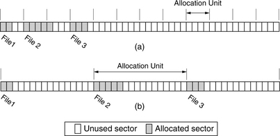
FIGURE 19.10 Effect of allocation unit size on small files: (a) 4-sector allocation unit size and (b) 16-sector allocation unit size.
• Most disk drives today do lookahead prefetch (this will be discussed in detail in Chapter 22) into a buffer whenever possible, allowing quick servicing of sequential or nearly sequential data requests in the near future. When a file occupies only a small portion of an allocation unit, prefetch is filling the lookahead buffer with mostly useless data from unused sectors, rendering prefetching less effective.
19.5 Concentric Tracks vs. Spiral Track
We will now revisit the issue of concentric tracks versus spiral track formatting first described in Chapter on data organization Chapter 18, Section 18.2. With the understandings that we have gained so far up to this point, we can now examine some of the design issues facing this choice of formatting.
As mentioned earlier, concentric tracks have always been the formatting used by magnetic disk drives, including removable media types such as floppy disks and the 3.5” diskettes. The major reasons for this are partly historical and partly ease of implementation. In the early days of disk drives, when open-loop mechanical systems were used to position the head, using discrete concentric tracks seemed the natural choice. Today, the closed-loop embedded servo system provides on track head positioning guidance, making spiral track formatting feasible. Nonetheless, concentric tracks are a well-understood and well-used technology and seems easier to implement than spiral track. Servo writing (placing of servo information on a disk at the time of manufacturing) for spiral track seems more complicated and will require new study and perhaps new invention ideas to make it practical. Therefore, unless there is some compelling advantages that spiral track offers, it will not likely be adopted by magnetic disk drives.
Spiral track does have a couple of advantages:
Formatting efficiency Concentric tracks have discrete track boundaries. The capacity of each track is fixed, dictated by the BPI and the radial position of the track, in accordance to
track capacity = 2 × π × radius × bpi (EQ 19.19)
However, since each track must hold an integer number of fixed-size sectors, there is a quantization effect, rendering some of the capacity of a track to be unavoidably wasted. Take a simple example where the capacity of some track, after discounting for servo wedges, is 420,000 bytes. Assume a sector, including all the overheads, is 602 bytes in length; then this track can hold 697 such sectors for a total of 419,594 bytes, effectively losing 406 bytes in capacity. Granted, this seems like a small number compared to the capacity of a track; nonetheless, if there are, say, 100,000 such tracks in the drive, 40 MB are lost.
Things get worse for concentric tracks when zoned-bit recording (ZBR) is applied. The track at the OD of a zone is recorded at a lower bpi than at the ID of that same zone, resulting in a loss in capacity equal to the difference between the track capacities of this zone and of the next outer zone.
If each concentric track is allowed to record at the maximum bpi, subject to the limitation of the quantization effect, then on average each track would lose half a sector of capacity. However, because magnetic disk drives rotate at a fixed speed, known as constant angular velocity (CAV) recording, this would require the drive to be able to handle an almost continuous spectrum of data rates. This is not yet practical.
Spiral track clearly does not have to deal with the quantization effect afflicting concentric tracks
Sustained data rate As discussed in the section on data rate, in the chapter on data organization, the drive must incur a head switch time or a cylinder switch time when going from the end of one concentric track to the beginning of the next logical track. The switch time is basically to position either the same head or a different head onto a new track. This causes a hiccup in the continuous flow of data. When transferring a large amount of sequential data, the sustained data is reduced from the number of user bytes per track x revolutions per second to

where THS is the head switch time, TCS is the cylinder switch time, and N is the number of heads.
If spiral track formatting is used, there is no end of one track and start of another track. Data just flows continuously from one sector to the next. Hence, when accessing sequential data, there is no head switching to speak of, and there is no reduction in sustained data rate, which is simply
data ratesustained = SPT × 512 × rpm / 60 (EQ 19.21)
Here, “SPT” is really the number of sectors encountered by the head in one full revolution, and it can be a fractional number since spiral track does not have the quantization restriction of concentric tracks, as we just discussed. Therefore, for the sequential type of data access, spiral track formatting has a data rate advantage over concentric tracks.
19.5.1 Optical Disks
Unlike magnetic disk drives, certain optical recordings such as CDs and DVDs have adopted the spiral track formatting. The playback of audio CDs and move DVDs operates in a constant linear velocity (CLV) mode in which a constant data transfer rate is maintained across the entire disk by moving the spiral track under the optical head at a fixed speed. This means the rotational speed varies depending on the radial position of the head, slower toward the OD and faster toward the ID. For example, a DVD rotates at roughly 1400 rpm at the ID, decreasing to 580 rpm at the OD.
While CLV recording is fine for long sequential reads and writes, it gives poor performance for random accesses because of the need to change the rotational speed which is a comparatively slow mechanical process. This is one of the reasons why the CLV recording method has never been adopted by magnetic disk drives. The constant data rate delivery of CLV recording fits well for audio/video applications, and those applications have little demand for high random-access performance. A fixed data rate also makes the read channel electronics simple, which matches well with the low-cost objective of mass market consumer electronics.
As various forms of recordable CDs and DVDs have been added for computer data storage applications, higher performance becomes a requirement. The 1 × CLV speed of a DVD only delivers a paltry data transfer rate of 1.32 MB/s, a far cry from the 40+ MB/s of today’s magnetic disks. To deliver a higher data transfer rate, drives for these recordable optical disks rotate at speeds many times faster than their consumer electronics brethren. For example, a 16× DVD operates at a competitive speed of 21.13 MB/s. In addition to rotating faster, DVD recorders employ a variety of operating modes to deliver higher performance. In addition to the CLV mode, they also use the CAV mode and the Zoned Constant Linear Velocity (ZCLV) mode. In ZCLV, the spiral track formatted disk is divided into zones. One method, as employed by DVD+R or DVD+RW, uses a different CLV speed for each zone. This only approximates the behavior of CAV, as the rotational speed still varies within each zone in order to maintain a constant linear speed. For instance, an 8× ZCLV DVD recorder might write the first 800 MB at 6× CLV and the remainder at 8× CLV. Another ZCLV method, as employed by DVD-RAM, uses a constant rotational speed within each zone, but varies that speed from zone to zone, faster toward the ID and slower toward the OD. This provides a roughly constant data rate throughout the whole disc, thus approximating the behavior of CLV.
19.6 Average Seek
As mentioned in the beginning of this chapter, seek time and rotational latency time are the biggest components of an I/O request that require a disk access. Since all magnetic disk drives rotate at a constant rpm, the average rotational delay is simply one-half the time of one disk revolution. The average seek time, however, is more complex and will be revisited and examined in greater detail here. The analysis given here is for purely random accesses, where every single sector in the drive is accessed with equal probability.
19.6.1 Disks without ZBR
We begin by making the simplifying assumption that the next I/O request resides in any cylinder with equal probability. This assumption is true only for disks with a constant number of sectors per track and not true for disks with ZBR. Consider a drive with C cylinders. The maximum seek distance, or full stroke seek, is then C – 1 cylinders. The probability of a 0 cylinder seek, i.e., the next request is for the current cylinder that the actuator is at, is simply 1/C. There are C2 possible combinations of a start cylinder and an end cylinder, of which 2(C – s) combinations will yield a seek distance of exactly s cylinders. Thus, the probability mass function for the discrete random variable s is 2(C – s)/C2. The average seek distance can be calculated by

which is approximately equal to (C – 1)/3 for a large value of C. So, if all cylinders have equal probability of access, the average seek distance is 1/3 the maximum seek, which has been used in the literature for many decades.
Some people use the average seek distance to determine the average seek time, i.e., they assume the average seek time to be the time to seek the average distance. However, this is not correct because, as discussed in Section 19.2.3, the relationship between the seek time and seek distance is not linear. To simplify the mathematics for determining the true average seek time, we will resolve the average seek distance in Equation 19.22, this time using s as a continuous random variable. This method is accurate because the number of cylinders in a drive is a very large number, typically in the tens of thousands. Furthermore, for the remainder of this section, the full stroke seek distance is normalized so that s is expressed as a fraction of the maximum seek distance and has a value between 0 and 1.
The position of a cylinder can also be expressed as a fraction of the maximum seek distance. Let x and y be two random variables representing a starting cylinder position and an ending cylinder position. The seek distance s when seeking from x to y is simply |x – y|. By symmetry, the seek distance when seeking from y to x is also |x – y|. Hence, without loss of generality, it can be assumed that x ≤ y.
To determine the mean value of s, it is necessary to have its density function f(s). To do that, we first determine its distribution function F[s] = Prob[seek distance [s] = 1 – Prob[s [ seek distance]. With the assumption of x [y, to produce a seek distance that is greater than or equal to s, x must be less than or equal to 1 – s, and y must be at least x + s. Hence,
where f(x) and f(y) are the density functions for x and y. With the assumption that every cylinder has an equal probability of being accessed, the density function for both x and y is simply 1, giving
The density function for s is simply
The mean seek distance can now be determined to be
which is the same result as that obtained before using s as a discrete random variable.
For disk drives employing the bang-bang method of seek, the seek profile can be expressed as
where A is the settle time component of the seek, B is some constant related to acceleration as indicated in Equation 19.11, and s is the normalized seek distance. Since the settle time is a constant in this simple model, we can study only the effect of seek distance on the travel time. For the case where every cylinder has an equal probability of being accessed, the average travel time can be computed using the seek distance density function f(s) of Equation 19.25:
Compare with B ![]() , which is the travel time for the mean 1/3 seek distance that some mistakenly use as the mean travel time; the incorrect method overestimates the real mean travel time by 8.25%.
, which is the travel time for the mean 1/3 seek distance that some mistakenly use as the mean travel time; the incorrect method overestimates the real mean travel time by 8.25%.
Next, consider the case for seek with a maximum speed limit. Let a be acceleration and T, as previously defined in Section 19.2.3, be the time required to reach maximum speed. Then, from Equations 19.11 and 19.12, the travel time for a seek distance of s is
The average travel time can now be calculated, again using the density function f(s) of Equation 19.25, as
which, with a little bit of work, can be solved to be
Continuing with the example of Section 19.2.3, which normalizes the acceleration a to a unit of 1 and selects T = 0.5 with such a unit, the weighted average travel time is 1.127 units. In comparison, the travel time for covering the average seek distance of 1/3 is, from Equation 19.29, 1.167 units, which is a 3.5% overestimation. It can be concluded that with either the bang-bang seek or the speed limited seek, the approximate method of using the seek time for 1/3 the maximum seek distance as the average seek time gives a reasonably accurate estimate, with an error of less than 10% of the true weighted average.
19.6.2 Disks with ZBR
So far, the assumption has been used that all cylinders are accessed with equal probability, which is the case for disks not using ZBR. The results and equations thus derived are not accurate for today’s drives, since all disks today use ZBR. With ZBR, tracks or cylinders nearer the OD have more sectors than those closer to the ID and, therefore, have higher probability of being accessed if all sectors in the drive are accessed equally.
To simplify the analysis, we will assume that the entire recording surface is recorded at the same areal density, as in the ideal case. Then the distribution function for a cylinder’s position is simply proportional to the recording area:
The maximum seek distance is (OD – ID)/2. Let k be the ratio of OD to ID. Furthermore, if the full stroke seek distance is normalized to 1, then
Substituting OD = k × ID and Equation 19.33 into Equation 19.32 results in
The density function for cylinder position x is simply
Next, the distribution function for the seek distance s of a ZBR disk can now be calculated by substituting the density function of Equation 19.35 for starting and ending cylinder positions x and y of Equation 19.23. With some work, the solution turns out to be
Figure 19.11 is a plot of this distribution function for a value of k = 3.5 and that of Equation 19.24 which is for no ZBR. Even for a ratio as large as 3.5, the two distribution functions are surprisingly close. This means that treating ZBR disks as non-ZBR disks in most performance analysis is, in general, an acceptably close approximation.

Taking the derivative of F[s] produces the density function
Finally, the average seek distance for a ZBR disk can be computed by substituting Equation 19.37 into
Figure 19.12 plots this average seek distance as a function of k. Note that this average for ZBR disks is lower than the average of 1/3 of full stroke seek for non-ZBR drives. This is as expected since it is less likely to access the tracks toward the ID.

To determine the average travel time for ZBR disks, again consider the case for bang-bang seek. Substituting Equation 19.37 for f(s) into
This is plotted in Figure 19.13 as a function of the OD to ID ratio k, with the full stroke seek time normalized to 1. Also plotted are the normalized travel time of for traversing the average normalized seek distance of ![]() and the normalized average travel time of 8/15 for non-ZBR disks. For k = 3, the travel time for 1/3 the maximum seek is off by more than 10% from the ZBR weighted average travel time.
and the normalized average travel time of 8/15 for non-ZBR disks. For k = 3, the travel time for 1/3 the maximum seek is off by more than 10% from the ZBR weighted average travel time.

Computing the average travel time of ZBR disks for speed limited seek is left as an exercise for motivated readers.