
Operational Performance Improvement
In many systems the access speed to data is the limiting factor for the performance of the entire system. While a disk drive with a given electro-mechanical design comes with certain raw performance characteristics that cannot be changed, such as its revolution time and seek profile, operation of the drive by its controller can bring about some differences in user-observable performance. Some of these techniques may also be implemented at the operating system level, in the form of data placement and scheduling algorithms. However, the drive controller, having detailed information about all the drive’s parameters (e.g., formatting) and its current states (e.g., position of the head), usually has an advantage in applying such techniques.
Once a user request has been received by a disk drive, it has some latitude in how to handle the request. A disk drive can take advantage of this limited degree of freedom to determine how best to perform the command, as long as it is transparent to the user and the command is satisfied correctly. In fact, the drive can even change the size, shape, and location of a user’s stored data as long as the drive is able to guarantee that the original data can be returned to the user. This chapter will explore some of the strategies available for handling a user’s data and commands to improve a disk drive’s overall performance. Not all strategies are good for all environments and situations. Some of the strategies make sense only for certain types of workload or under certain circumstances.
21.1 Latency Reduction Techniques
As discussed in Chapter 19, rotational latency is a major time component of any I/O which is not part of a sequential access. Besides the obvious approach of increasing rpm, which is fixed for a given design and not for the drive controller to change freely, there are several other methods for reducing rotational latency [Ng 1991]. Unfortunately, all of these methods are costly to implement.
21.1.1 Dual Actuator
One method for a drive to reduce rotational latency is to add a second set of read/write heads and actuator [Ng 1994b]. The actuator would be placed such that the second set of heads operate 180o from the original set of heads, as illustrated in Figure 21.1. When a read or a write request is to be serviced, the controller sends both actuators to the target track. Both actuators should arrive at the destination at roughly the same time. Based on the servo ID of the first servo wedge encountered (from either head), the drive controller can determine which head is rotationally closer to the target sector and use that head to service the read or write request. The rotational delay is between zero and one-half of a disk revolution with a constant distribution. Hence, the average rotational latency is reduced from the one-half revolution standard case to one-fourth of a revolution.
This is a clean solution for latency reduction, but it is also an expensive solution. The addition of a second set of heads and actuator increases the cost of the drive by about 30–40%. The highly price competitive nature of the disk drive business makes this solution economically not very viable. Conner Peripherals introduced such a product called Chinook in 1994, but it failed to take off, and no other drive makers have attempted to produce such a design since.
21.1.2 Multiple Copies
A second approach to reducing rotational latency of I/O accesses is to maintain two or more complete copies of data on the drive.1 For ease of discussion, dual copy is discussed here—extension to multiple copies is straightforward. Every sector of data is arranged such that it and its duplicate copy are located 180o out of phase with respect to each other. In other words, if a copy is currently under the head, its second copy is half a revolution away from the head. There are multiple ways with which this can be implemented. One method is to divide each track into two halves. The data recorded on the first half of a track is repeated in the second half. This means that each track should have an even number of sectors. With this approach, the number of logical tracks in a cylinder is not changed, but the capacity of each track is reduced by a factor of two. An alternative method is to pair up the heads in the actuator of the drive, assuming that there are an even number of heads. Data on the tracks of the odd-numbered heads are duplicated on the tracks of the corresponding even-numbered heads, with the start (first sector) of the odd tracks offset by 180° from the start of the even tracks. With this approach, the number of logical tracks in a cylinder is halved, but the capacity of each track is not changed.
With either method of data layout, any requested data always has one copy that is within half a revolution from the head. For reading, this cuts the average rotational latency to one-fourth of a revolution. Unfortunately, for writing, two copies of the same data must be written. Although the average rotational latency for reaching the closest copy is one-fourth of a revolution, the write is not completed until the second copy is written. Since the second copy is half a revolution away, the average rotational latency for writes effectively becomes three-fourths of a revolution. The resulting net average rotational latency for all I/O accesses is
revolution, where fR is the fraction of I/Os being reads. Thus, whether rotational latency is reduced or increased depends on the read-to-write ratio of the users’ access pattern.
While no additional hardware is required with the dual copy approach, the capacity of the drive is reduced by one-half. This essentially doubles the dollar per gigabyte of the drive. In some high-end server applications, where the storage capacity per drive is deliberately kept low for performance reasons (drives are added to a system for the arms rather than capacity), a drive’s capacity is not fully used anyway. For such environments, there is less or even no real increase in cost to the user. The only cost is then that of having to pay a higher performance penalty for writes.
21.1.3 Zero Latency Access
While there is some increased cost associated with the previous two methods for rotational latency reduction, a third approach carries no added cost and, hence, is implemented in many of today’s disk drives. However, this method only benefits large I/O requests, providing little or no improvement for those I/O requests with small block sizes. This approach, called zero latency read/write (also sometimes referred to as roll-mode read/write), employs the technique of reading or writing the sectors of a block on the disk out of order. Since this method works in the same way for reads and for writes, reads will be used for discussion here.
Traditionally, after a head has settled on the target track, the drive waits for the first sector of the requested block to come around under the head before data access is started. This is true regardless of whether the head first lands outside the block or inside the block. With zero latency read (ZLR), the head will start reading the next sector it encounters if it lands inside the requested block. Consider an example where the requested block is half a track’s worth of data, all of which resides on the same track. Assume that the head lands right in the middle of this block. A traditional access method would require the drive to wait for 3/4 of a revolution for the beginning of the block to arrive under the head and then take another 1/2 revolution to retrieve the block, for a total of 1¼ revolutions to complete the request. With ZLR, the drive will first read the second half of the block,2 wait for one-half of a revolution for the beginning of the block to come around, and then take another one-fourth of a revolution to retrieve the remainder (first half) of the requested block. This entire process takes only one full revolution, saving one-fourth of a revolution compared to the traditional method. In essence, the effective rotational latency is reduced. If the head lands outside the requested block, ZLR works in the same way as the traditional method.
In general, let B be the block size in number of sectors. For the case where the block resides all on one track, the probability of landing inside the block is p = B/SPT, which is also the fraction of a track being requested. The total rotational time to access the block is one disk revolution. Since the data transfer time is B/SPT of a revolution, this means an effective rotational latency of (1 – B/SPT) of a revolution. The probability of landing outside the block is (1 – p), and the average rotational latency for this case is (1 – B/SPT)/2 revolutions. Therefore, the average rotational latency is
of a revolution. This is plotted in Figure 21.2. When p is very small, the average rotational latency is about 1/2, as expected. When p approaches 1, the latency is effectively reduced to 0 with this technique.

Next, consider the case where the requested block crosses a track boundary and resides in two consecutive tracks. Let D be the track switch time (either head switch or cylinder switch) expressed in number of sectors. If B is the number of sectors of the requested block that resides on the first track, and C is the number of remainder sectors of the requested block that resides on the second track, then the requested block size is equal to B + C. There are two cases to consider:
1. Requested block size is less than (SPT – 2D). ZLR can be made to work to produce the same result as when the entire block is on a single track. As shown in Figure 21.3(a), when the head lands inside the requested block of the first track, it can start reading to retrieve the middle portion of the block, switch to the second track to read the last portion of the block, and then switch back to the first track to complete reading the initial portion of the block. Because there is sufficient time and spacing for track switches, the whole process can be completed in one disk revolution. Hence, for this case, Equation 21.2 and Figure 21.2 can be applied.

FIGURE 21.3 Zero latency access procedure for requested block spanning two tracks. Step 1: Read middle portion of block from first track. Step 2: Switch to second track. Step 3: Read last portion of block from second track. Step 4: Switch back to first track. Step 5: Wait for start of block to come around. Step 6: Read first portion of block from first track. (a) Requested block < SPT – 2D. (b) SPT – 2D < requested block < 2 × SPT – 2D.
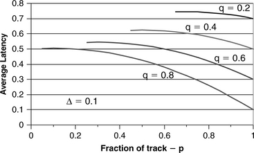
2. Requested block size is greater than (SPT – 2D), but less than (2 × SPT – 2D). Let the fraction of the first track being requested be p = B/SPT, the fraction of the second track being requested be q = C/SPT, and Δ = D/SPT. When the head lands inside the requested block on the first track, with probability p, it can be seen in Figure 21.3(b) that it takes two revolutions of disk rotation time to complete the data access if ZLR is employed. The data transfer time is (B + D + C)/SPT = p + q + Δ revolutions, which means the effective rotational latency is (2 – (p + q + Δ)) revolutions. The probability of landing outside the block is (1 – p), and the average rotational latency in this case is (1 – B/SPT)/2 = (1 – p)/2 revolutions. Therefore, the average rotational latency is

of a revolution. This is plotted in Figure 21.4 for q = 0.2, 0.4, 0.6, and 0.8. A value of 0.1 is chosen for D, which is typical. It can be observed from Figure 21.4 that except for large values of p + q, ZLR in this case actually performs worse than not doing ZLR. A simple strategy for the disk drive controller to implement can be to turn on ZLR in this case only when q exceeds a certain threshold, say, 0.7.
When the requested block spans more than two tracks, all the tracks in the middle require one full revolution plus track switch to access, so it does not make any difference whether ZLR is used or not. Only the first track and last track need to be examined. Therefore, the preceding analysis can be applied—just substitute the last track for the second track in the above.
21.2 Command Queueing and Scheduling
For a long time, it was common for the host to issue a single I/O command to a disk drive and wait for that request to be completed before giving the disk drive the next I/O command. Even today, ATA drives, which are the predominant type of disk drives sold in 2005, operate in this mode. The host CPU makes use of the long waiting time for an I/O request to be completed by switching tasks to perform some other activities for another program or application. The widening of the gap between the speed of CPU and that of disk drive over the years has been dealt with by increasing the level of multi-programming so as to keep the overall throughput of the system up.
It would be a more efficient use of a disk drive’s capability if the host presented to the drive a list of I/O requests that need to be serviced and let the disk drive decide the most efficient order of servicing those commands. This is indeed the rationale behind command queueing and reordering. In command queueing, a unique tag ID is assigned to each I/O request issued by the host and sent to the drive as part of the command structure. When the drive has completed a command, the host is notified using this tag so that the host knows which of the many outstanding I/O requests is done. The host is free to reuse this tag ID for a new command.
The number of commands outstanding in a disk drive is called the queue depth. Clearly, the longer the queue depth is, the more choices are available for the drive to optimize, and the more efficient command reordering will be. Host-disk interface standards define an upper limit for the allowable queue depth. For SATA, this limit is 32. For SCSI, it is 256; however, the host and disk drive usually negotiate for some smaller value at the disk drive’s initialization time. Even though performance improves with queue depth, the percentage of improvement decreases with queue depth so that beyond a certain point there is little benefit in increasing the queue depth. Sorting the queue to select the next command requires computation, and this is done while the drive is servicing the current command. Ideally, this computation should be overlapped with the drive’s seek and rotational times so that it does not add any visible overhead. This may not be achievable if a very long queue needs to be sorted. For these two reasons, limited gain and excessive computation, queue depth should be kept to some reasonable number. What is reasonable depends on the computational complexity of the sorting algorithm chosen and the processing power of the drive’s microprocessor.
With command queueing, the drive has the flexibility to schedule the ordering of execution of the commands for better performance. The benefit of command reordering is that the average service time of an I/O is reduced, which means the net through put of the disk drive is increased. As discussed in Chapter 20, seek time and rotational latency time are the two major components of a random I/O’s time. Thus, command reordering that can result in reducing one or both of these components will be able to improve the overall throughput of the disk drive.
The response time of an I/O request is the time from when the command is sent to the disk drive to when the disk drive has completed servicing the command and signals back to the host of the completion. This time includes the time for the actual servicing of the command and the time of the command sitting in the command queue waiting for its turn to be serviced. For a First-Come-First-Serve (FCFS) scheduling policy, commands are serviced in the order of their arrival, i.e., there is no reordering, and the waiting time of an I/O is simply the total service times of all the other I/O requests in front of it in the queue. While command reordering will reduce the average response time since the average service time of I/Os is reduced, there will be a greater variance in response time. Some I/Os that just arrive may get selected for servicing quickly, while others may sit in the queue for a long time before they get picked.
Typically, with command reordering, some kind of aging algorithm needs to be put in place so that no I/O will wait for an unduly long time. In fact, most host-disk interfaces require an I/O to be completed within some time limit or else the host will consider an error condition has occurred. An aging policy increases the selection priority of a request as it ages in the queue so that after some time it gains the highest selection priority for execution.
In the following, several of the most common scheduling algorithms will be described [Geist & Daniel 1987, Seltzer et al. 1990, Worthington et al. 1994, Thomasian & Liu 2002, Zarandioon & Thomasian 2006]. Typical implementations are usually some variations or enhancements of one of these algorithms. Normal operation is to redo or update the command sorting each time a new command arrives at the queue. This has the overall best performance, but can lead to a long delay for some I/Os. One compromise variation is to sort on only the first N commands in the queue until all of them are executed, and then the next group of N commands are sorted and executed. This trades off efficiency for guaranteeing that no command will be delayed for more than N – 1 I/Os.
21.2.1 Seek-Time-Based Scheduling
Earlier scheduling policies are a class of algorithms which are based on reducing seek time. Since seek time monotonically increases with seek distance, the algorithms simply operate on seek distance reduction techniques. Furthermore, because in early systems the host was cognizant of the geometry of an attached disk drive, it was possible to perform this type of scheduling at the host level instead of inside the disk drive. Later, even when logical addressing was introduced to replace physical addressing on the host-disk interface, due to the fact that with traditional (meaning, not serpentine) data layout there is a linear relationship between the logical address and physical location, host scheduling was still feasible. Today, with the disk drive’s internal data layout scheme unknown to the host, such as the serpentine formatting described in Chapter 18, Section 18.3.3, it makes more sense to do the scheduling inside the drive.
SSTF One seek time based scheduling algorithm is called the Shortest-Seek-Time-First. As its name implies, it searches the command queue and selects the command that requires the least amount of seek time (or equivalently, seek distance) from the current active command’s position. SSTF is a greedy policy, and the bad effect is that it tends to favor those requests that are near the middle of the disk, especially when the queue depth is high. Those requests near the OD and ID will be prone to starvation. An aging policy definitely needs to be added to SSTF.
LOOK Also called Elevator Seek. In this algorithm, the scheduling starts from one end of the disk, say, from the outside, and executes the next command in front of (radially) the actuator’s current position as it works its way toward the inside. So, it is doing SSTF in one direction—the direction that the actuator is moving. New commands that arrive in front of the current actuator position will get picked up during the current sweep, while those that arrive behind the actuator position will not be selected. As the drive finishes the radially innermost command in the queue, the actuator will reverse direction and move toward the OD, and scheduling will now be done in the outward direction. Since all commands in the queue are guaranteed to be visited by the actuator in one complete cycle, no aging policy is required.
C-LOOK Even though LOOK is a more fair scheduling algorithm than SSTF, it still favors those requests that are near the middle of the disk. The middle of the disk is visited twice in each cycle, whereas the outside and inside areas are visited only once. To address this, the Circular-LOOK algorithm schedules only in one direction. Thus, when the actuator has finished servicing the last command in one direction, it is moved all the way back to the farthest command in the opposite direction without stopping. This trades off some efficiency for improved fairness.
21.2.2 Total-Access-Time-Based Scheduling
The previous group of scheduling policies is based on reducing seek time only. Although, on average, that is better than no reordering, it is not the most effective way to reduce total the I/O time since it ignores the rotational latency component of an I/O. A command with a short seek may have a long rotational delay and, hence, a longer total access time than another command which requires a longer seek but a shorter rotational delay. This is clearly illustrated in Figure 21.5. A scheduling policy based on minimizing the total access time, defined as the sum of seek time and rotational latency time, is called Shortest-Access-Time-First (SATF) or Shortest-Positioning-Time-First (SPTF) [Jacobson & Wilkes 1991, Worthington et al. 1994, Ng 1999]. Some people also use the term Rotational Position Optimization (RPO). All disk drives today that support command queueing use SATF reordering because of its superior performance over policies that are based on seek time only. Just like SSTF, SATF is a greedy algorithm; it simply selects from among the commands in the queue the one that can be accessed the quickest as the next command to be serviced.
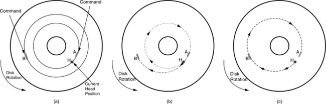
FIGURE 21.5 Scheduling policies. (a) Two commands in queue. Command A is on the same track as the current head position, but has just rotated pass it. Command B is on a different track. (b) Seek time based policy. Command A is selected next, ahead of command B. It takes almost one-and-a-half revolutions to service both A and B. (c) Access time-based policy. Command B is selected ahead of command A. It takes less than one revolution to service both A and B.
As a new I/O arrives at the drive’s command queue, its starting LBA is translated into a CHS physical address. The cylinder number represents its radial position, and the sector number represents its angular position. This translation is done only once, and the physical address information, which is needed for estimating the command’s access time each time the queue is sorted, is stored with the command.
Estimating Access Time
To sort the command queue for SATF selection, a direct approach would be to estimate for each command its seek time and the ensuing rotational latency, and then sum them up. The reference position for such calculations is from the current active command’s expected ending position. A reasonably accurate seek profile would be needed, unlike seek time-based policies which can sort by seek distance in place of seek time. The seek profile is generally stored as a piece-wise linear table of seek times for a number of seek distances. The number of seek table entries is relatively small compared to the number of cylinders in the drive so as to keep the table size compact. Because the seek time tends to be fairly linear for large seek distances, as discussed in Chapter 19 and illustrated in Figure 19.6, the seek table entries typically are focused on shorter seek distances and become sparse as the seek distance increases. Seek time for any seek distance can be calculated using linear interpolation. Rotational latency is straightforward to estimate as the drive rotates at a constant rpm.
The constant rotation of the disk has a quantization effect in the sense that a given sector comes directly under the head at a regular interval, which is once every revolution. This fact can be taken advantage of to simplify the access time calculation. The expected ending position of the currently active command can be computed based on its starting LBA and the block size. The difference in radial position between this ending position and the starting position of a command in the queue can be used to estimate the seek time, tseek, for that command by using the seek table. Similarly, a rotation time, trotation, can be calculated from the difference in angular positions (this total rotation time is not to be confused with rotational latency, which is the rotation time after the seek has been completed). If tseek is less than trotation, then taccess = trotation; otherwise, the time of one or more disk revolution, trevoiution, has to be added until tseek < trotation + n · trevoiution. This is a smarter way than the direct method of computing how much rotation has occurred during tseek, figuring out how much more rotation needs to take place, and then computing the rotational latency.
Simplified Sorting Methods
The preceding procedure for estimating access time needs to be carried out for each command to be sorted in order to determine which command has the shortest access time. While this is the most accurate method, it is also somewhat computationally intensive, and if there are many commands in the queue, there may not be enough time to sort through all of them before the currently active command is completed. There are various methods to simplify the sorting by trading off some degree of preciseness.
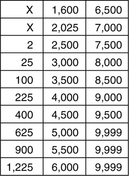
One method is to divide angular positions evenly into N buckets. If N = 10, then each bucket accounts for 36° of a disk’s angular positions, and if there are 1000 sectors in a track, the first 100 sectors belong to the first bucket, the next 100 sectors belong to the next bucket, etc. The larger N is, the more precise this method; the trade-off is between access time estimation accuracy and table space. In practice, the number of servo wedges in a drive is a sensible and practical choice for N, since the no-ID table can be used to identify which servo ID. (SID) a sector belongs to. In this case, a bucket would correspond to a SID. However, such a choice is optional and not required for this scheme to work. Each command in the queue is placed in one of these buckets according to its starting angular position. A table with N entries is created for the drive at manufacturing time. Each entry corresponds to an angular distance in terms of the buckets. For example, the sixth entry is for angular positions that are five buckets away; the first entry is for zero distance. The first column of this table is for the maximum seek distances that can be reached within the rotational times of the corresponding angular distances. Thus, the sixth entry in this first column is the maximum seek distance reachable within the time for rotating to an angular position that is five buckets away. The second column of the table is for the maximum seek distances that can be reached within the rotational times of the corresponding angular distances plus the time of one complete disk revolution. This continues until the full stroke seek distance is reached in the table.
Figure 21.6 shows an example of such a table with N = 10 for a hypothetical disk with 10,000 cylinders. To use this table, after the current command has started, the drive controller determines the expected ending position of the current command. Say, its angular position belongs in the i-th bucket. The controller looks in the (i + 1) bucket, modulo N, to see if it contains any queued command. If the bucket is empty, it goes to the next bucket, then the bucket after that, etc., until a non-empty bucket is found. Let’s say this is the (i + k) bucket. It then checks each command in that bucket to see if its seek distance relative to the ending position of the current command is less than the k-th entry of the first column of the RPO table. If an entry that satisfies this criteria can be found, then the sorting is done. This is rotationally the closest command that can also be seeked to within the rotational time. All previously examined commands are rotationally closer than this one, but none of them can have their seeks completed within their rotational times. Hence, this is going to be the command with the shortest access time. All other remaining commands will require longer rotational time and do not need to be examined. If no entry in the bucket can satisfy the seek criteria, then move on to the next bucket and continue searching. When k has reached N – 1 and still no selectable command is found, the process is repeated, this time using the second column of the table, and so on.
Performance Comparison
The effectiveness of command queueing for disk drives that support it is often measured in terms of the maximum achievable throughput at various queue depths. The command queue is kept at a given queue depth for the measurement of each data point. Thus, when an I/O is completed, a new one is immediately added back to the queue. The typical workload chosen for doing comparisons is pure random I/Os of small block sizes over the entire address range of the disk drive. This is the most demanding workload, and it is representative of one that would be observed for drives used in a multi-user server environment, such as on-line transaction processing (OLTP) which demands high performance from disk drives. Sequential accesses, while also an important class of workload, are less demanding and exercise other aspects of a drive’s capability such as caching.
It is intuitive that SATF policy should outperform policies that are based only on seek time. Command reordering is not amenable to analytical solutions. Determining the effectiveness of a particular policy requires either simulation or actual measurement on a working disk drive which has that policy implemented. In this section, some simulation results based on random number generation are discussed.
A hypothetical disk drive with an OD to ID ratio of 2.5 and 1000 SPT at the OD is assumed. It uses a simple bang-bang seek with A = 0.5 and B = 10 for normalized seek distances. Hence, according to Chapter 19, Equations 19.27 and 19.41, the average seek time is 5.75 ms. The workload is pure random reads of 1 KB blocks. Non-overlapped controller overhead is negligible and ignored here. Initially, a rotation speed of 10K rpm is chosen; later it will be varied to study the effect of rpm. It can be easily computed that without reordering the average I/O time is 5.75 ms + 3 ms (average latency) + 0.016 ms (average data transfer time) = 8.766 ms. Thus, with FCFS scheduling, this drive is capable of handling 114 IOPS (I/Os per second).
Figure 21.7 shows the simulated throughput of SSTF, C-LOOK, and SATF for various queue depths. One million I/Os are simulated for each data point. The superiority of SATF is clearly demonstrated. One point of interest is that at low queue depth SSTF outperforms C-LOOK, while at high queue depth the two have essentially identical throughput.
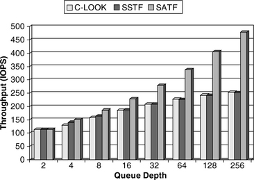
As the queue depth is increased, it can be expected that eventually a point of diminishing return would be reached as the throughput approaches the theoretical maximum. For seek time based scheduling, the minimum I/O time would be 0.5 ms for settling + 3 ms average latency + 0.016 ms data transfer time, yielding an upper bound throughput of 284 IOPS. Indeed, the gain for SSTF and C-LOOK in going from a queue depth of 128 to 256 has slowed down to 4.5% compared to the gain in throughput of 6.6% of going from 64 to 128. On the other hand, the upper bound for SATF is much higher as it can also eliminate rotational latency when there is an infinite number of commands in the queue. The theoretical maximum throughput for SATF is 1938 IOPS. The 478 IOPS at a queue depth of 256 is still far below this upper bound, and, hence, the point of diminishing return is nowhere in sight yet.
Practical Issues of SATF
So far, the discussion has been on the theoretical aspect of SATF with simple idealized conditions. Here, some real-world practical issues facing the actual implementation of SATF in a disk drive are discussed.
Seek Time Variability This is the practical issue that has the biggest impact on SATF scheduling. Since SATF is based on minimizing the sum of seek time and latency time, a selected command may have a very short latency component. For such a command, there is little room for error in performing the seek. If the seek actually takes longer than estimated to complete, it may consume all the projected latency time, and the target sector may just have passed by. In this case, the drive must wait a full disk revolution before it can access the data. This situation, called a miss revolution, is a very costly error. This will not happen if the actuator servo can produce seek times that are precisely repeat-able all the time so that the controller can make accurate seek time projection in scheduling for SATF. Unfortunately, due to a number of factors, some of which may not even be in the control of the servo, there will always be some degree of variation in the seek time. These factors include vibration, operating temperature, transient errors while reading a servo ID, etc.
To deal with this seek time variance by being conservative and allowing a good margin for the seek time may not be the most optimum solution. Even though this would avoid the misrevolution penalty completely, it also leads to missing out on some better selections which have a good chance of completing on time. Being overly aggressive in scheduling based on an optimistic seek profile, one that does not have a high percentage of making the seek in time, would also be bad, obviously, due to paying the miss revolution penalty too frequently. Thus, a good compromise strategy should be adopted. Simulation seems to suggest that a scheduling that results in roughly 3–4% miss revolutions yields the best overall throughput.
One method for handling seek time variance in SATF scheduling is to modify the estimated access time according to the probability of its seek being successfully on time. Thus, if a seek has a probability p of not completing in tseek, then its contribution to access time is computed to be
tseek + p × trevolution (EQ 21.4)
An example of how this enhancement in assessing the cost of an I/O can be added to the earlier discussed simplified sorting method is as follows. Instead of just one seek distance number in each entry in the RPO table, as illustrated in Figure 21.6, there are M distances, d1, d2, …, dM per table entry. d1 represents the distance below which a seek is 100% likely to complete within the rotational time associated with the corresponding bucket, dM represents the distance above which a seek has 0% chance of completing. A distance between di and di+1 has a (M – i)/M probability of completing in the available time. When searching through the command queue as described before, if a command is found k-th bucket away from the current I/Os bucket, and this command has a distance d which is between di and di+1 of the k-th table entry, then the access cost function (in terms of buckets) of this command is
where N is the number of buckets. The minimum estimated cost of all the commands examined so far is remembered. When a first command is encountered such that its seek distance is less than the d1 of its corresponding table entry (100% seek completion probability), its cost function is compared with the minimum cost computed so far. The command with the lower estimated cost is selected to be the next command. All remaining commands do not need to be examined.
To illustrate this algorithm, the previous example, in which N = 10, is expanded using M = 4, and the new RPO table is shown in Figure 21.8; only the first column is shown for brevity. Assume the ending position of the currently active command is in bucket 35. Search the command queue, which is presorted by bucket, starting at bucket 37. The first non-empty bucket is, say, bucket 40, and it has one command with a seek distance of 196 cylinders from the current active command. Looking at the sixth entry in the table, 196 is between d1 (180) and d2 (212). Hence, it has a 3/4 probability of completing the seek, and its access cost (in terms of buckets) is
(40 – 35) + 1/4 × 10 = 7.5 (EQ 21.6)
Since this is the first command examined, it is remembered as the lowest cost command so far. Assume the next non-empty bucket is bucket 42, and it has one command with a seek distance of 513. Since 513 is smaller than d1 (565) of the eighth entry in the table, it has 100% of completing in time. The estimated access cost of this command is therefore simply 42 – 35 = 7. Since this is the first command with a seek distance less than d1, its cost is compared to the minimum cost computed so far, which is 7.5. This newly examined command in bucket 42 has a smaller cost and is thus selected to be the next command. Other commands in the queue do not need to be checked. In contrast, if the simple table of Figure 21.6 is used, the command in bucket 40 would have been selected.
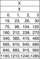
FIGURE 21.8 Example of an expanded RPO table based on angular distance. M = 4, and only the first column is shown.
Environmental Change A change in the operating environment of the disk drive, such as temperature, can cause the seek characteristics of the drive to change. Therefore, it is important to continually monitor the drive’s seek behavior and adjust its seek profile or the RPO table accordingly.
Workload While the previous discussion on performance comparison assumed a pure random workload, many real-world workloads are a mix of random and sequential accesses. While doing scheduling, care must be taken to ensure that two sequential commands that are in a command queue get scheduled and executed back to back without missing a revolution. This is discussed in more detail in Section 21.2.3.
Priority The discussions on scheduling so far have been assuming that all I/O requests are of the same priority. If supported by the interface, some commands may arrive at the queue at a higher priority. Such commands need to be serviced first even though they may not be optimal selections from a performance viewpoint. Furthermore, for drives operating in certain environments, such as attached to a storage controller which has non-volatile write caching, write commands received by the drive are only for destaging from the controller’s write cache and have no effect on the host system’s performance, whereas read requests, on the other hand, are needed by host’s applications and therefore their response times can affect such applications’ performance. For such environments, it makes sense to give read commands higher priority than writes, even if such priority is not explicitly specified by the host, provided the read is not for a sector of one of the outstanding write commands. This can be accomplished by multiplying the estimated access time of writes with a weighing factor greater than 1 or adding to it some fixed additional time. For example, multiplying with a factor of 2 means that a write command will not be selected unless its estimated access time is less than half of that of the fastest read.
Aging As mentioned earlier, some sort of aging algorithm needs to be added on top of SATF to ensure that no command waits in the command queue for an unduly long time. One simple way is to have a counter for each command which is initialized to zero on its arrival at the queue. Each time a selection is made from the queue, the counters of all other commands in the queue are incremented. The estimated access time for a command is then adjusted by subtracting this counter multiplied by some fixed number. The result of adding aging is that the variance in response time is reduced, but overall throughput will also be slightly decreased.
N-Step Lookahead SATF is a Greedy algorithm as it always selects the pending request with the shortest estimated access time as the next command for servicing. Some simulation studies have shown that an alternative approach of looking ahead so that the sum of the estimated access times for the next N commands is the shortest can produce somewhat better performance. The event that can invalidate the tenet of this approach is when a new arrival results in a whole different sequence of optimal commands. For example, command sequence ABCD has been selected, and after A has been completed, command G arrives. If it was known that G was going to arrive, a better sequence would have been ECGF, and so selecting A to be executed next was not the best choice after all. The probability of this happening increases with N and when the workload is heavy. The computational complexity of this approach also goes up exponentially with N. For these two reasons, N should probably be kept small.
21.2.3 Sequential Access Scheduling
In Chapter 19, Section 19.1.1, the importance of the sequential type of accesses in increasing the effective performance of a disk drive was explained, since such an access could be completed faster than one that involved a seek and a rotational latency by an order of magnitude. Thus, for a drive to deliver good performance, it is imperative that it be able to handle properly various kinds of sequential accesses, as defined in Chapter 19, Section 19.1.1, so as not to miss out on the opportunity of short service time accorded by such I/O requests.
Regardless of which scheduling policy is used, the drive controller must ensure that if there are two commands in the queue and their addresses are sequential, then they get scheduled and executed back to back without missing any revolutions. This means the controller should coalesce all sequential or near-sequential commands before execution of the first command in the sequence is started. The commands need to be coalesced because starting a new command involves a certain amount of overhead which is substantially longer than the rotation time of the gap between two sectors. Thus, if the two sequential commands are not coalesced and executed as one, the second command will suffer a misrevolution. Ideally, the drive also should have the capability to extend a currently executing command to access more data. This is so that if a new command arrives and it is sequential to the currently active command, it can be handled immediately and efficiently.
A good drive controller should also be able to handle skip sequential commands in a similar manner. Since the command overhead can be the rotation time of multiple sectors, it is also necessary to coalesce such commands. While this is not a problem for reads, as the controller can simply read the not requested sectors along with the requested sectors into the drive’s buffer, it is a problem for writes since the write buffer does not contain the data for the skipped sectors. This can be handled by using a skip mask. By setting the appropriate bits in a special register, the drive controller can signal to the write channel electronics which sectors to write and which sectors to skip. For instance, a mask of 111000011111 would signal to write three sectors starting at the command’s LBA, then skip four sectors, and then write the next five sectors after that.
21.3 Reorganizing Data on the Disk
It is a fact that related data are generally accessed together, either all at once or within a very small window of time. Examples of related data are the blocks of a file, the source code of a program and its header files, or all the boot-time startup modules. This spatial and temporal locality of access is the basis of many strategies for improving disk drive performance. As pointed out previously, sequential accesses can be completed much more quickly than accesses that require a seek and rotational latency. Therefore, one class of strategies is to locate related data physically together so that it can be accessed more efficiently. Any such data layout reorganization activity should be done in the background and, preferably, during lull periods in the disk drive or storage system so that the performance of regular user requests is not affected.
Since the content of data blocks is known to the file system, e.g., “this file consists of these eight blocks” or “these twelve files are all in the same sub-directory and therefore are likely to be related,” this class of strategies is best handled at wherever the file manager is located, which today is in the host system. The drive, lacking such higher level information, is less suitable. Nonetheless, there are still a few things that the drive controller may be able to do, especially since it knows the internal geometry of the drive which the host does not know. Also, there are classes of files, such as databases, large files, memory-mapped files, etc., where not all blocks are necessarily accessed together, and, hence, the lack of file system knowledge is not a big drawback.
21.3.1 Defragmentation
The first obvious thing to do with regard to related data is to locate all the blocks of a file in contiguous address space. Generally, this is the case when starting out with a fresh system or when creating a new file in a drive that has lots of not-yet used space. Depending on the file system, each time a file grows, its growth blocks may be located somewhere else if the original blocks are not to be moved. This leads to the file being fragmented. Also, after the system has gone through many file allocations and deallocations, the disk address space may be left with many small holes, and it may be difficult to find contiguous space to fit a new large file. The result is, again, a fragmented file. Over time, the performance of a disk drive will degrade if the percentage of fragmented files goes up. The solution to this problem is to perform defragmentation. During this process, all the blocks of each fragmented file are gathered together and relocated to a new contiguous address space. At the same time, the files are repacked together so as to squeeze out all the holes so that the drive ends up with one large free space available for future new file allocations. This may involve moving some of the files more than once. Defragmentation is one form of data reorganization.
21.3.2 Frequently Accessed Files
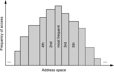
Another form of data reorganization is to relocate those files that are most frequently accessed close together. While this does not help to increase the fraction of sequential accesses, it helps reduce the overall average seek distance as the head moves only short distances from one frequently accessed file to another, which should occur more often on average. Additionally, by locating these files in the middle of all the cylinders, roughly halfway between OD and ID (skewed toward the OD for ZBR), it also reduces the average seek from any random location on the disk to one of these files, from roughly one-third of full stroke to one-fourth. For this method, the file access frequencies need to be monitored and the collected data used periodically to dynamically reorganize the file locations. A classical algorithm for placing these files is to locate the most frequently accessed file in the logical center of the drive, where the LBA is one-half the drive’s total number of sectors. The other frequently accessed files, in descending order of frequencies, are next placed on either side of it, alternating from one side to the other, as shown in Figure 21.9. This is known as the organ pipe arrangement, for obvious reasons [Knuth 1973].
Data reorganization imposes a great deal of extra work on the disk drive. The previous set of frequently accessed files first needs to be moved out from their central locations, then the new set of frequently accessed files is moved into those vacated locations. To reduce the amount of work, one strategy is to not migrate newly identified frequently accessed files out of their present location. Instead, they are duplicated in the central location of the disk. The advantage is that since the original copy of each file is always in its permanent location, there is no need to move out data from the central location. It can simply be overwritten; only the file system table needs to be updated. However, now there are two copies of those files. There are two options for handling a write to one of these files. One choice is to write to both copies of the file, which doubles the amount of work to be done. A second choice is to write only to the permanent copy of the file and invalidate the second copy in the file system table, making the second and more conveniently located copy no longer available for access. Neither solution is ideal, and which one is better depends on the ratio of writes to reads for that file. If write is more dominant, then it is better to forfeit the second copy. If read is more dominant, then it is better to update both copies so that the more frequent reads can benefit from faster access.
While disk drives do not yet have file system awareness,3 they can adopt the data reorganization technique of relocating frequently accessed data close together on a block basis rather than on a file basis. However, it may not be practical, as the overhead of monitoring access frequency on a block basis may be too great for the resource-constrained drive controller to handle.
21.3.3 Co-Locating Access Clusters
Certain files tend to be accessed together. Furthermore, they are accessed in exactly, or almost exactly, the same sequence each time. For such files, it makes sense to relocate them permanently so that they are stored together in the disk drive as a cluster and in the order with which they are likely to be accessed. In this way, each time they are accessed, they can be accessed efficiently as some form of sequential access. One good example and candidate of this class of data reorganization is the boot sequence of a system. Various boot optimizers have been developed which learn how a system is configured to boot up. After the system has been booted a few times, the optimizer is able to determine the likely sequence with which various files and applications are loaded from the disk drive into the system memory. It then sees to it that these files get co-located accordingly. Application loadings are another class of candidates for this strategy, with programs called application launch accelerators as the counterpart to boot optimizers.
21.3.4 ALIS
The Automatic Locality-Improving Storage (ALIS) methodology [Hsu and Smith 2004, Hsu et al. 2005] combines both the strategy of relocating frequently accessed data together and the strategy of co-locating an observed common sequence of data accesses. It calls the first strategy heat clustering (data that is frequently accessed is said to be hot) and the second strategy run clustering (run as in “a continuous sequence of things”). Data monitoring and reorganization are performed at a block level, not on a file basis. Hence, it can be implemented either in the host or in the disk drive if the drive has enough resources such as computational power and temporary storage to do so. Fixed-size blocks are the reorganization units, with the block size being a design parameter.
Heat Clustering
ALIS recognizes that the organ pipe organization of data, whose goal is to reduce the average seek distance, has these shortcomings:
• A small amount of seek is not that much saving over a slightly longer seek.
• It has the tendency to move the head back and forth across the central most frequently accessed file as it accesses hot files on both sides of it.
• Rotational latency is not reduced.
• The concept was born of an era when disk I/Os were basically first come first serve. With today’s command queueing and reordering, this approach provides little, if any, benefit.
• It was not designed to take advantage of the prefetching that is commonly performed today both in the host cache and in the drive cache.
Instead of organ pipe data placement, ALIS recommends a heat clustering strategy of simple sequential layout, whereby the hot data blocks identified for duplication are arranged in a reserved reorganization area in the order of their original block addresses. The underlying theory of this strategy is to retain the sequentiality of the original data, but with those data that are inactive filtered out. In a typical real workload, only a small fraction (empirical measurements indicate about 15%) of a disk’s total data is normally in active use.
Run Clustering
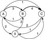
ALIS also takes advantage of the fact that in most real workloads there are long read sequences that are often repeated due to certain tasks being asked to be performed repeatedly. Launching a common application is one such example. To identify such runs, ALIS constructs an access graph to continuously keep track of I/O request sequencing. Each vertex of the graph represents a block, and the edge from vertex i to vertex j represents the desirability for locating block j after block i. Each time block j is accessed within k commands of accessing block i, the value of the edge from vertex i to vertex j is incremented by t – k + 1 if k ≥ t, where t is a design parameter called the context size. A context size greater than 1 is needed to make allowance for a user’s request stream being intermixed with other users’ request streams, as in a multi-programming or a server environment. Figure 21.10 illustrates a simple example of such an access graph for the block sequence ABCAXBC with t = 2. Since the number of blocks in a drive is likely to be huge for any sensible block size, the size of the access graph needs to be kept to some reasonable maximum size by pruning. Edges with low weights and vertices whose edges are all with low weights are dropped. To enable old patterns to exit the graph gracefully and not become stagnant, an aging algorithm is added to the edge weights.
To identify a run for clustering from an access graph, first select the edge with the highest weight; its two vertices form the seed of the run. Next, find and add to the run the vertex whose edges to all the vertices in the run have the highest weight sum. This can be a vertex that gets added to the beginning or to the end of the run. This continues until the length of the run exceeds t, the context size. From this point on, the head of the run is defined to be the first t vertices of the run, and the tail of the run is defined to be the last t vertices. Continue to grow by iteratively finding and adding to the run the vertex whose edges to either the head or the tail have the highest weight sum. Finally, this growth process terminates when the head weight and the tail weight fall below some threshold. This threshold is another ALIS design parameter. Figure 21.11 shows a highly simplified example of this process in identifying the run ABCDE from an original reference stream of ABCDEABXCDE.

Cluster Selection During Service Time
Heat clustering and run clustering co-exist in the reorganization space. A block may appear multiple times in different clusters. Hence, when an I/O request arrives, there may be choices as to which cluster to use for servicing the request. Because runs are specific patterns of access that are likely to be repeated, they are selected first. If a matching run cannot be found, then heat clusters are searched. When still no match can be found, then it is necessary to use the original copy of the data as no duplicate of the data exists.
21.4 Handling Writes
In some environments, write commands arrive at the disk drive in bursts. One such example is when there is write caching at the host or storage controller, which periodically destages all the writes that have been cached to the disk drive. Furthermore, the writes are random writes that update data scattered throughout the drive, with each write requiring a seek and a rotational latency. To service all the writes of a burst can tie up the drive for some time, even if a command reordering technique is used to minimize the mechanical times, thus affecting the response time of any read command that comes during this period.
The class of strategies designed to handle this situation is, again, based on the observation that sequential accesses are a lot faster than random accesses. The general idea is that, instead of updating the individual write data in its original locations, all the new data is written together in a sequential string to some new location. A directory or relocation table must be maintained to point to the location of every piece of data in the drive. Sections 21.4.1 and 21.4.2 discuss two strategies for batching the writes as one sequential access.
21.4.1 Log-Structured Write
When this method is implemented at the host level, it is known as the log-structured file system (LFS). A similar technique can also be applied at the disk level by the drive controller, transparently and unbeknown to the host. In this method, the disk address space is partitioned into fixed-size segments, with each segment containing many sectors. This segment size is a design parameter. A certain number of free segments must be available at all times, one of which is being used as the active write segment. When a sufficient number of writes requests (e.g., enough data to fill a segment) have accumulated at the level where this log-structured write is implemented, the new data are all written out together sequentially to the active write segment, starting at the next available sector. A log of these individual writes is appended to the end of this new sequence of data. Each log entry contains the original LBA of each write and the LBA of its new location.
An in-memory directory is updated with the same information as the log. Once the directory is updated, references to the old copies of data are gone, basically invalidating the old data and freeing up its space. It may be desirable to keep a list of such free spaces or how much free space each segment has so that future cleanup can be expedited. The directory is periodically, and also during normal shut down, saved to the disk at a fixed known location. When the drive and the system are next started up, the directory can be read back in to memory. The purpose of the logs is for reconstructing the directory since its last known good state should the drive or system be shut down abnormally, such as during a power interruption. The disk drive maintains a flag which indicates whether it was powered down properly or unexpectedly. All systems also have a similar status indicator.
The main advantage of this log-structured write strategy is that many random small writes are turned into a long sequential write which can be completed very quickly. However, it comes with the following disadvantages:
• An originally contiguous piece of data will be broken up when part of it gets an update write. The more writes it goes through, the more fragmented it becomes. Thus, if the user reads the data, what was once data that could be accessed with a single sequential read now becomes many random reads. Thus, this strategy makes sense only for workloads that are dominated by small writes.
• Because of the holes created in segments by writes invalidating data in previous locations, they need to be consolidated so as to create new empty segments for new writes, in a process known as garbage collection. This is extra work that the drive needs to take care of, and in a heavily used system, there may not be sufficient idle times for this function to be performed non-intrusively.
• The disk drive needs to have a sizable amount of excess capacity, as much as 20%, over the total amount of actual data stored so that it does not run out of free segments too frequently. In this way, it can have more leeway in scheduling when to do garbage collection.
• Address translation for an I/O request must now go through one more level of indirection, adding extra overhead to each command.
• All data in a log-structured storage would be lost if its directory is lost or corrupted. The system must be carefully designed so that the directory can be recovered or reconstructed if needed. Reconstruction of the directory will be a time-consuming process.
Because of these shortcomings, log-structured writes should not be, and have not been, implemented in a general-purpose disk drive. Even for heavy write environments where this strategy may make sense, either at the system or at the drive level, careful design considerations and trade-offs should be evaluated before deciding on adopting this strategy.
Finally, if ALIS or some other usage-based clustering technique is used in conjunction with a log-structured write, data reorganization can be opportunistically performed during the garbage collection process. As valid data needs to be consolidated to create full segments, those data that are discovered to belong to the same heat cluster or run cluster can be placed in the same segment.
21.4.2 Disk Buffering of Writes
This method can be considered to be doing a partial log-structured write and only on a temporary basis. While it may be possible to implement this strategy at the host level, it is more practical to implement it inside the disk drive. In this technique, the drive has a small amount of reserved space dedicated to this function, preferably divided into a few areas scattered throughout the drive. Similar to a log-structured write, when a sufficient number of write commands have been accumulated, all these random writes are gathered and written out to one of these areas, preferentially the one that is closest to the current head position, as one long sequential write. Again, a log of these writes is appended to the end. This is where similarity with the log-structured write ends.
Here, relocation of data is only temporary. The home location of each piece of data is not changed—just its content is temporarily out of date. In other words, the disk has been used to buffer the writes. During idle periods in the disk drive, the drive controller reads back the buffered data and writes each of them to its home location. In essence, the drive delays all the random writes from a time when the drive is busy with other concurrent read requests requiring fast response time to a time when no user requests are waiting to be serviced and so the long completion time of random writes does not matter. While the amount of work that the drive ends up doing is increased, the apparent performance of the drive to the user is improved. Furthermore, since the update data is eventually written back to its home location, the long-term sequentiality of a user’s data does not get damaged over time—an important advantage over the log-structured write strategy. A small directory or relocation table is needed to properly point to where the temporarily buffered data is located. LBAs not listed in the relocation table can be found in their home locations.
21.5 Data Compression
When data is first compressed before storing to the disk, more data can be stored. Compressing the data can be performed either at the host level, at the storage subsystem controller level, or inside the disk drive. If data can be compressed at an average compression ratio of C to 1, then, in essence, the storage capacity of the disk drive is increased C times. In addition to this seemingly marvelous attribute, data compression can also potentially improve performance. First, the media transfer rate is effectively increased C folds. Second, the track capacity is increased C times, reducing or even eliminating seek distances between a user’s data. (Refer back to Chapter 19, Section 19.2.1, for a more in-depth discussion of performance impact of a larger track capacity.)
However, data compression has a few major issues.
• Data compression is computationally intensive, although using a dedicated compression chip or hardware can alleviate the problem.
• The compression ratio is highly data content sensitive. Some data compresses well, while other data cannot be compressed at all. Furthermore, a piece of data will likely be compressed to a different size each time its content is changed. Thus, when data is modified, its new compressed output may no longer fit in the space previously allocated to that data. One solution is to use compression in conjunction with the log-structured write, since the log-structured write does not write back to the original location and, hence, the size of the data does not matter. Another solution is to allocate some slack space for each piece of compressed data so as to minimize the probability of not being able to fit a modification back into the allocated space. For those rare occasions when the modification does not fit, then the data is relocated to some new space.
• If multiple pieces of compressed data are packed into a sector, then modifying any one of them and writing it back will require a read-modify-write of the sector. This degrades performance very substantially as the process requires a read, waiting basically one revolution, and then a write. Again, the log-structured write can be a solution to this problem.
1Using multiple copies of data on multiple drives, such as mirroring or RAID-1, also works and is discussed in Section 24.2 of Chapter 24.
2In this discussion, the average one-half sector delay for reading the first available sector is ignored, since it is only a very small fraction of a revolution.
3This is a concept that has been discussed for many years, but has not materialized yet.