
DRAM Device Organization: Basic Circuits and Architecture
In this chapter, basic circuits and architecture of DRAM devices are described. Modern DRAM devices exist as the result of more than three decades of devolutionary development, and it is impossible to provide a complete overview as well as an in-depth coverage of circuits and architecture of various DRAM devices in a single chapter. The limited goal in this chapter is to provide a broad overview of circuits and functional blocks commonly found in modern DRAM devices, and then proceed in subsequent chapters to describe larger memory systems consisting of DRAM devices composed of the commonly found circuits and functional blocks described herein.
This chapter proceeds through an examination of the basic building blocks of modern DRAM devices by first providing a superficial overview of a Fast Page Mode (FPM) DRAM device. Basic building blocks such as DRAM storage cells, DRAM array structure, voltage sense amplifiers, decoders, control logic blocks, data I/O structures, and packaging considerations are examined in this chapter. Specific DRAM devices, such as SDRAM, DDR SDRAM and D-RDRAM devices, and the evolution of DRAM devices, in general, are examined in Chapter 12.
8.1 DRAM Device Organization
Figure 8.1 illustrates the organization and structure of an FPM DRAM device that was widely used in the 1980s and early 1990s. Internally, the DRAM storage cells in the FPM DRAM device in Figure 8.1 are organized as 4096 rows, 1024 columns per row, and 16 bits of data per column. In this device, each time a row access occurs, a 12-bit address is placed on the address bus and the row-address strobe (RAS)1 is asserted by an external memory controller. Inside the DRAM device, the address on the address bus is buffered by the row address buffer and then sent to the row decoder. The row address decoder then accepts the 12-bit address and selects 1 of 4096 rows of storage cells. The data values contained in the selected row of storage cells are then sensed and kept active by the array of sense amplifiers. Each row of DRAM cells in the DRAM device illustrated in Figure 8.1 consists of 1024 columns, and each column is 16 bits wide. That is, the 16-bit-wide column is the basic addressable unit of memory in this device, and each column access that follows the row access would read or write 16 bits of data from the same row of DRAm.2

In the FPM DRAM device illustrated in Figure 8.1, column access commands are handled in a similar manner as the row access commands. For a column access command, the memory controller places a 10-bit address on the address bus and then asserts the appropriate column-access strobe (CAS#) signals. Internally, the DRAM chip takes the 10-bit column address, decodes it, and selects 1 column out of 1024 columns. The data for that column is then placed onto the data bus by the DRAM device in the case of an ordinary column read command or is overwritten with data from the memory controller depending on the write enable (WE) signal.
All DRAM devices, from the venerable FPM DRAM device to modern DDRx SDRAM devices, to high data rate XDR DRAM devices to low-latency RLDRAM devices, to low-power MobileRAM devices, share some basic circuits and functional blocks. In many cases, different types of DRAM devices from the same DRAM device manufacturer share the exact same cells and same array structures. For example, the DRAM cells in all DRAM devices are organized into one or more arrays, and each array is arranged into a number of rows and columns. All DRAM devices also have some logic circuits that control the timing and sequence of how the device operates. The FPM DRAM device shown in Figure 8.1 has internal clock generators as well as a built-in refresh controller. The FPM DRAM device keeps the address of the next row that needs to be refreshed so that when a refresh command is issued, the row address to be refreshed can be loaded from the internal refresh counter instead of having to be loaded from the off-chip address bus. The inclusion of the fresh counter in the DRAM device frees the memory controller from having to keep track of the row addresses in the refresh cycles.
Advanced DRAM devices such as ESDRAM, Direct RDRAM, and RLDRAM have evolved to include more logic circuitry and functionality on-chip than the basic DRAM device examined in this chapter. For example, instead of a single DRAM array in an FPM DRAM device, modern DRAM devices have multiple banks of DRAM arrays, and some DRAM devices have additional row caches or write buffers that allow for read-around-write functionality. The discussion in this chapter is limited to basic circuitry and architecture, and advanced performance-enhancing logic circuits not typically found on standard DRAM devices are described separately in discussions of specific DRAM devices and memory systems.
8.2 DRAM Storage Cells
Figure 8.2 shows the circuit diagram of a basic one-transistor, one-capacitor (1T1C) cell structure used in modern DRAM devices to store a single bit of data. In this structure, when the access transistor is turned on by applying a voltage on the gate of the access transistor, a voltage representing the data value is placed onto the bitline and charges the storage capacitor. The storage capacitor then retains the stored charge after the access transistor is turned off and the voltage on the wordline is removed. However, the electrical charge stored in the storage capacitor will gradually leak away with the passage of time. To ensure data integrity, the stored data value in the DRAM cell must be periodically read out and written back by the DRAM device in a process known as refresh. In the following section, the relationships between cell capacitance, leakage, and the need for refresh operations are briefly examined.

Different cell structures, such as a three-transistor, one-capacitor (3T1C) cell structure in Figure 8.3 with separate read access, write access, and storage transistors, were used in early DRAM designs.3 The 3T1C cell structure has an interesting characteristic in that reading data from the storage cell does not require the content of the cell to be discharged onto a shared bitline. That is, data reads to DRAM cells are not destructive in 3T1C cells, and a simple read cycle does not require data to be restored into the storage cell as they are in 1T1C cells. Consequently, random read cycles are faster for 3T1C cells than 1T1C cells. However, the size advantage of the 1T1C cell has ensured that this basic cell structure is used in all modern DRAM devices.

Aside from the basic 1T1C cell structure, research is ongoing to utilize alternative cell structures such as the use of a single transistor on a Silicon-on-Insulator (SOI) process as the basic cell. In one proposed structure, the isolated substrate is used as the charge storage element, and a separate storage capacitor is not needed. Similar to data read-out of the 3T1C cell, data read-out is not destructive, and data retrieval is done via current sensing rather than charge sensing. However, despite the existence of alternative cell structures, the 1T1C cell structure is used as the basic charge storage cell structure in all modern DRAM devices, and the focus in this chapter is devoted to this dominant 1T1C DRAM cell structure.
8.2.1 Cell Capacitance, Leakage, and Refresh
In a 90-nm DRAM-optimized process technology, the capacitance of a DRAM storage cell is on the order of 30 fF, and the leakage current of the DRAM access transistor is on the order of 1 fA. With a cell capacitance of 30 fF and a leakage current of 1 fA, a typical DRAM cell can retain sufficient electrical charge that will continue to resolve to the proper digital value for an extended period of time—from hundreds of milliseconds to tens of seconds. However, transistor leakage characteristics are temperature-dependent, and DRAM cell data retention times can vary dramatically not only from cell to cell at the same time and temperature, but also at different times for the same DRAM cell.4 However, memory systems must be designed so that not a single bit of data is lost due to charge leakage. Consequently, every single DRAM cell in a given device must be refreshed at least once before any single bit in the entire device loses its stored charge due to leakage. In most modern DRAM devices, the DRAM cells are typically refreshed once every 32 or 64 ms. In cases where DRAM cells have storage capacitors with low capacitance values or high leakage currents, the time period between refresh intervals is further reduced to ensure reliable data retention for all cells in the DRAM device.
8.2.2 Conflicting Requirements Drive Cell Structure
Since the invention of the 1T1C DRAM cell, the physical structure of the basic DRAM cell has undergone continuous evolution. DRAM cell structure evolution occurred as a response to the conflicting requirements of smaller cell sizes, lower voltages, and noise tolerances needed in each new process generation. Figure 8.4 shows an abstract implementation of the 1T1C DRAM cell structure. A storage capacitor is formed from a stacked (or folded plate) capacitor structure that sits in between the polysilicon layers above active silicon. Alternatively, some DRAM device manufacturers instead use cells with trench capacitors that dive deeply into the active silicon area. Modern DRAM devices typically utilize one of these two different forms of the capacitor structure as the basic charge storage element.
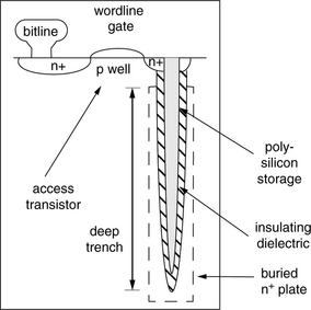
FIGURE 8.4 Cross-section view of a 1T1C DRAM cell with a trench capacitor. The storage capacitor is formed from a trench capacitor structure that dives deeply into the active silicon area. Alternatively, some DRAM device manufacturers instead use cells with a stacked capacitor structure that sits in between the polysilicon layers above the active silicon.
In recent years, two competing camps have been formed between manufacturers that use a trench capacitor and manufacturers that use a stacked capacitor as the basic charge storage element. Debates are ongoing as to the relative costs and long-term scalability of each design. For manufacturers that seek to integrate DRAM cells with logic circuits on the same process technology, the trench capacitor structure allows for better integration of embedded DRAM cells with logic-optimized semiconductor process technologies. However, manufacturers that focused on stand-alone DRAM devices appear to favor stacked capacitor cell structures as opposed to the trench capacitor structures. Currently, DRAM device manufacturers such as Micron, Samsung, Elpida, Hynix, and the majority of the DRAM manufacturing industry use the stacked capacitor structure, while Qimonda, Nanya, and several other smaller DRAM manufacturers use the trench capacitor structure.
8.2.3 Trench Capacitor Structure
Currently, the overriding consideration for DRAM devices, in general, and commodity DRAM devices, in particular, is that of cost-minimization; This over-riding consideration leads directly to the pressure to reduce the cell size—either to increase selling price by putting more DRAM cells onto the same piece of silicon real estate or to reduce cost for the same number of storage cells. The pressure to minimize cell area, in turn, means that the storage cell either has to grow into a three-dimensional stacked capacitor above the surface of the silicon or has to grow deeper into and trench below the surface of the active silicon. Figure 8.4 shows a diagram of the 1T1C DRAM cell with a deep trench capacitor as the storage element. The abstract illustration in Figure 8.4 shows the top cross section of the trench capacitor.5 The depth of the trench capacitor allows a DRAM cell to decrease the use of the silicon surface area without decreasing storage cell capacitance. Trench capacitor structures and stacked capacitor structures have respective advantages and disadvantages. One advantage of the trench capacitor design is that the three-dimensional capacitor structure is under the interconnection layers so that the higher level metallic layers can be more easily made planar. The planar characteristic of the metal layers means that the process could be more easily integrated into a logic-optimized process technology, where there are more metal layers above the active silicon. The buried structure also means that the trench capacitor could be constructed before logic transistors are constructed. The importance of this subtle distinction means that processing steps to create the capacitive layer could be activated before logic transistors are fabricated, and the performance characteristics of logic transistors would not be degraded by formation of the (high-temperature) capacitive layer.6
8.2.4 Stacked Capacitor Structure
The stacked capacitor structure uses multiple layers of metal or conductive polysilicon above the surface of the silicon substrate to form the plates of the capacitor to form the plates of the capacitor that holds the stored electrical charge. Figure 8.5 shows an abstract illustration of the stacked capacitor structures. The capacitor structure in Figure 8.5 is formed between two layers of polysilicon, and the capacitor lies underneath the bitline. It is referred to as the Capacitor-under-Bitline (CUB) structure. The stacked capacitive storage cell can also be formed above the bitline in the Capacitor-over-Bitline (COB) structure. Regardless of the location of the storage cell relative to the bitline, both the CUB and COB structures are variants of the stacked capacitor structure, and the capacitor resides in the polysilicon layers above the active silicon. The relentless pressure to reduce DRAM cell size while retaining cell capacitance has forced the capacitor structure to grow in the vertical dimension, and the evolution of the stacked capacitor structure is a natural migration from two-dimensional plate capacitor structures to three-dimensional capacitor structures.

8.3 RAM Array Structures
Figure 8.6 illustrates an abstract DRAM array in a top-down view. The figure shows a total of six cells, with every two cells sharing the same bitline contact. The figure also abstractly illustrates the size of a cell in the array. The size of a unit cell is 8 F2. In the current context, “F” is a process-independent metric that denotes the smallest feature size in a given process technology. In a 90-nm process, F is literally 90 nm, and an area of 8 F2 translates to 64,800 nm2 in the 90-nm process. The cross-sectional area of a DRAM storage cell is expected to scale linearly with respect to the process generation and maintains the cell size of 6∼8 F2 in each successive generation.

In DRAM devices, the process of data read out from a cell begins with the activation of the access transistor to that cell. Once the access transistor is turned on, the small charge in the storage capacitor is placed on the bitline to be resolved into a digital value.7 Figure 8.7 illustrates a single bank of DRAM storage cells where the row address is sent to a row decoder, and the row decoder selects one row of cells. A row of cells is formed from one or more wordlines that are driven concurrently to activate one cell on each one of thousands of bitlines. There may be hundreds of cells connected to the same bitline, but only one cell per bitline will share its stored charge with the bitline at any given instance in time. The charge sharing process by the storage capacitor minutely changes the voltage level on the bitline, and the resulting voltage on the bitline is then resolved into a digital value by a differential sense amplifier. The differential sense amplifier is examined in the following section.

FIGURE 8.7 One DRAM bank illustrated: consisting of one DRAM array, one array of sense amplifiers, and one row decoder—note that the row decoder may be shared across multiple banks.
In modern DRAM devices, the capacitance of a storage capacitor is far smaller than the capacitance of the bitline. Typically, the capacitance of a storage capacitor is one-tenth of the capacitance of the long bitline that is connected to hundreds or thousands of other cells. The relative capacitance values create the scenario that when the small charge contained in a storage capacitor is placed on the bitline, the resulting voltage on the bitline is small and difficult to measure in an absolute sense. In DRAM devices, the voltage sensing problem is resolved through the use of a differential sense amplifier that compares the voltage of the bitline to a reference voltage.
The use of the differential sense amplifier, in turn, places certain requirements on the array structure of the DRAM device. In particular, the use of a differential sense amplifier means that instead of a single bitline, a pair of bitlines is used to sense the voltage value contained in any DRAM cell. Furthermore, in order to ensure that bitlines are closely matched in terms of voltage and capacitance values, they must be closely matched in terms of path lengths and the number of cells attached. These requirements lead to two distinctly different array structures: open bitline structures and folded bitline structures. The structural difference between an array with an open bitline structure and an array with a folded bitline structure is that in the open bitline structure, bitline pairs used for each sense amplifier come from separate array segments, while bitline pairs in a folded bitline structure come from the same array segment. The different structure types have different advantages and disadvantages in terms of cell size and noise tolerance. Some of the important advantages and disadvantages are selected for discussion in the following sections.
8.3.1 Open Bitline Array Structure
Figure 8.8 shows an abstract layout of an open bitline DRAM array structure. In the open bitline structure, bitline pairs used for each sense amplifier come from separate array segments. Figure 8.8 shows that the open bitline structure leads to a high degree of regularity in the array structure, and the result is that cells in an open bitline structure can be packed closely together. Typically, DRAM cells in an open bitline structure can occupy an area as small as 6 F2. In contrast, DRAM cells in a folded bitline structure typically occupy a minimum area of 8 F2.8 The larger area used by cells in a folded bitline structure is due to the fact that two bitlines are routed through the array for each DRAM cell in the folded bitline structure, while only one bitline is routed through the array for each cell in an open bitline structure.

Open bitline array structures were used in 64-Kbit and earlier DRAM generations. Some 256-Kbit DRAM devices also used open bitline structures. However, despite the advantage of smaller cell sizes, open bitline structures also have some disadvantages. One disadvantage of the open bitline structure is that it requires the use of dummy array segments at the edges of the DRAM array in order to ensure that the lengths and capacitance characteristics of the bitline pairs are closely matched. Another disadvantage of the classic open bitline structure is that bitline pairs in the open bitline array structure come from different array segments, and each bitline would be more susceptible to electronic noises as compared to bitlines in the folded bitline structure.
The larger area for routing and dummy array segments in open bitline structure minutely dilutes the cell size advantage of the open bitline structures. The various trade-offs, in particular, the noise tolerance issue, have led to the predominance of folded bitline structures in modern DRAM devices. Consequently, open bitline array structures are not currently used in modern DRAM devices. However, as process technology advances, open bitline structures promise potentially better scalability for the DRAM cell size in the long run. Research in the area of basic DRAM array structure is thus ongoing. Open bitline array structures or more advanced twisting or folding of the bitline structure with the cell size advantage of the open bitline architecture can well make a comeback as the mainstream DRAM array structure in the future.
8.3.2 Folded Bitline Array Structure
Figure 8.9 shows a DRAM array with a folded bitline structure. In the folded bitline configuration, bitlines are routed in pairs through the DRAM array structure, fulfilling several critical requirements of the sensitive differential sense amplifier. The close proximity of the bitline pairs in the folded bitline structure means that the differential sense amplifier circuit, when paired with this array structure, exhibits superior common-mode noise rejection characteristics. That is, in the case of a charge spike induced by a single event upset (SEU) neutron or alpha particle striking the DRAM device, the voltage spike would have a good chance of appearing as common-mode noise at the input of the differential sense amplifier. In the case of the open bitline array structure, the charge spike induced by the SEU would likely appear as noise on only one bitline of a bitline pair that connects to a sense amplifier.

Figure 8.9 shows a logical layout of the folded bitline structure where alternate pairs of DRAM cells are removed from an open bitline array. The array of DRAM cells is then compressed, resulting in the folded bitline structure illustrated in Figure 8.9. The folded bitline structure shown in Figure 8.9 is a simple twisting scheme where the bitline pairs cross over each other for every two transistors on the bitline. More advanced bitline folding schemes are being study to reduce the area impact while retaining the noise immunity aspect of the folded bitline structure.
8.4 Differential Sense Amplifier
In DRAM devices, the functionality of resolving small electrical charges stored in storage capacitors into digital values is performed by a differential sense amplifier. In essence, the differential sense amplifier takes the voltages from a pair of bitlines as input, senses the difference in voltage levels between the bitline pairs, and amplifies the difference to one extreme or the other.
8.4.1 Functionality of Sense Amplifiers in DRAM Devices
Sense amplifiers in modern DRAM devices perform three generalized functions. The first function is to sense the minute change in voltage that occurs when an access transistor is turned on and a storage capacitor places its charge on the bitline. The sense amplifier compares the voltage on that bitline against a reference voltage provided on a separate bitline and amplifies the voltage differential to the extreme so that the storage value can be resolved as a digital 1 or 0. This is the sense amplifier’s primary role in DRAM devices, as it senses minute voltage differentials and amplifies them to represent digital values.
The second function is that it also restores the value of a cell after the voltage on the bitline is sensed and amplified. The act of turning on the access transistor allows a storage capacitor to share its stored charge with the bitline. However, the process of sharing the electrical charge from a storage cell discharges that storage cell. After the process of charge sharing occurs, the voltage within the storage cell is roughly equal to the voltage on the bitline, and this voltage level cannot be used for another read operation. Consequently, after the sensing and amplification operations, the sense amplifier must also restore the amplified voltage value to the storage cell.
The third function is that the sense amplifiers also act as a temporary data storage element. That is, after data values contained in storage cells are sensed and amplified, the sense amplifiers will continue to drive the sensed data values until the DRAM array is precharged and readied for another access. In this manner, data in the same row of cells can be accessed from the sense amplifier without repeated row accesses to the cells themselves. In this role, the array of sense amplifiers effectively acts as a row buffer that caches an entire row of data. As a result, an array of sense amplifiers is also referred to as a row buffer, and management policies are devised to control operations of the sense amplifiers. Different row buffer management policies dictate whether an array of sense amplifiers will retain the data for an indefinite period of time (until the next refresh), or will discharge it immediately after data has been restored to the storage cells. Active sense amplifiers consume additional current above quiescent power levels, and effective management of the sense amplifier operation is an important task for systems seeking optimal trade-off points between performance and power consumption.
8.4.2 Circuit Diagram of a Basic Sense Amplifier
Figure 8.10 shows the circuit diagram of a basic sense amplifier. More complex sense amplifiers in modern DRAM devices contain the basic elements shown in Figure 8.10, as well as additional circuit elements for array isolation, careful balance of the sense amplifier structure, and faster sensing capability. In the basic sense amplifier circuit diagram shown in Figure 8.10, the equalization (EQ) signal line controls the voltage equalization circuit. The functionality of this circuit is to ensure that the voltages on the bitline pairs are as closely matched as possible. Since the differential sense amplifier is designed to amplify the voltage differential between the bitline pairs, any voltage imbalance that exists on the bitline pairs prior to the activation of the access transistors would degrade the effectiveness of the sense amplifier.

The heart of the sense amplifier is the set of four cross-connected transistors, labelled as the sensing circuit in Figure 8.10. The sensing circuit is essentially a bi-stable circuit designed to drive the bitline pairs to complementary voltage extremes, depending on the respective voltages on the bitlines at the time the SAN (Sense-Amplifier N-Fet Control) and SAP (Sense-Amplifier P-Fet Control) sensing signals are activated. The SAN signal controls activation of the NFets in the sensing circuit, and the SAP signal controls the activation of the PFets in the sensing circuit. After the assertion of the SAN and SAP, the bitlines are driven to the full voltage levels. The column-select line (CSL) then turns on the output transistors and allows the fully driven voltage to reach the output and be read out of the DRAM device. At the same time, the access transistor for the accessed cell remains open, and the fully driven voltage on the bitline now recharges the storage capacitor. Finally, in case of a write operation, the column-select line and the write enable (WE) signals collectively allow the input write drivers to provide a large current to overdrive the sense amplifier and the bitline voltage. Once the sense amplifier is overdriven to the new data value, it will then hold that value and drive it into the DRAM cell through the still open access transistor.
8.4.3 Basic Sense Amplifier Operation
The maximum voltage that can be placed across the access transistor is Vgs − Vt. (Vt is the threshold voltage of the access transistor, and Vgs is the gate-source voltage on the access transistor.) By overdriving the wordline voltage to Vcc + Vt, the storage capacitor can be charged to full voltage (maximum of Vcc) by the sense amplifier in the restore phase of the sensing operation. In modern DRAM devices, the higher-than-Vcc wordline voltage is generated by additional level-shifting voltage pumping circuitry not examined in this text.
Figure 8.11 shows four different phases in the sensing operations of a differential sense amplifier. The precharge, access, sense, and restore operations of a sense amplifier are labelled as phases zero, one, two, and three, respectively. The reason that the precharge phase is labelled as phase zero is because the precharge phase is typically considered as a separate operation from the phases of a row-access operation. That is, while the Precharge phase is a prerequisite for a row-access operation, it is typically performed separately from the row-access operation itself. In contrast, Access, Sense, and Restore are three different phases that are performed in sequence for the row-access operation.

Phase zero in Figure 8.11 is labelled as Precharge, and it illustrates that before the process of reading data from a DRAM array can begin, the bitlines in a DRAM array are precharged to a reference voltage, Vref. In many modern DRAM devices, Vcc/2, the voltage halfway between the power supply voltage and ground, is used as the reference voltage. In Figure 8.11, the equalization circuit is activated to place the reference voltage for the bitlines, and the bitlines are precharged to Vref.
Phase one in Figure 8.11 is labelled as (cell) Access, and it illustrates that as a voltage is applied to a wordline, that wordline is overdriven to a voltage that is at least Vt above Vcc. The voltage on the wordline activates the access transistors, and the selected storage cells discharge their contents onto the respective bitlines. In this case, since the voltage in the storage cell represents a digital value of “1,” the charge sharing process minutely increases the voltage on the bitline from Vref to Vref+. Then, as the voltage on the bitline changes, the voltage on the bitline begins to affect operations of the cross-connected sensing circuit. In the case illustrated in Figure 8.11, the slightly higher voltage on the bitline begins to drive the lower NFet to be more conductive than the upper NFet. Conversely, the minute voltage difference also drives the lower PFet to be less conductive than the upper PFet. The bitline voltage thus biases the sensing circuit for the sensing phase.
Phase two in Figure 8.11 is labelled Sense, and it illustrates that as the minute voltage differential drives a bias into the cross-connected sensing circuit, SAN, the DRAM device’s NFet sense amplifier control signal, turns on and drives the voltage on the lower bitline down.9 The figure shows that as SAN turns on, the more conductive lower NFet allows SAN to drive the lower bitline down in voltage from Vref to ground. Similarly, SAP, the PFet sense amplifier control signal, drives the bitline to a fully restored voltage value that represents the digital value of “1.” The SAN and SAP control signals thus collectively force the bi-stable sense amplifier circuit to be driven to the respective maximum or minimum voltage rails.
Finally, phase three of Figure 8.11 is labelled as Restore, and it illustrates that after the bitlines are driven to the respective maximum or minimum voltage values, the overdriven wordline remains active, and the fully driven bitline voltage now restores the charge in the storage capacitor through the access transistor. At the same time, the voltage value on the bitline can be driven out of the sense amplifier circuit to provide the requested data. In this manner, the contents of a DRAM row can be accessed concurrently with the row restoration process.
8.4.4 Voltage Waveform of Basic Sense Amplifier Operation
Figure 8.12 shows the voltage waveforms for the bitline and selected control signals illustrated in Figure 8.11. The four phases labelled in Figure 8.12 correspond to the four phases illustrated in Figure 8.11. Figure 8.12 shows that before a row-access operation, the bitline is precharged, and the voltage on the bitline is set to the reference voltage, Vref. In phase one, the wordline voltage is overdriven to at least Vt above Vcc, and the DRAM cell discharges the content of the cell onto the bitline and raises the voltage from Vref to Vref+. In phase two, the sense control signals SAN and SAP are activated in quick succession and drive the voltage on the bitline to the full voltage. The voltage on the bitline then restores the charge in the DRAM cells in phase three.

Figure 8.12 illustrates the relationship between two important timing parameters: tRCD and tRAS. Although the relative durations of tRCD and tRAS are not drawn to scale, Figure 8.12 shows that after time tRCD, the sensing operation is complete, and the data can be read out through the DRAM device’s data I/O. However, after a time period of tRCD from the beginning of the activation process, data is yet to be restored to the DRAM cells. Figure 8.12 shows that the data restore operation is completed after a time period of tRAS from the beginning of the activation process, and the DRAM device is then ready to accept a precharge command that will complete the entire row cycle process after a time period of tRP.
8.4.5 Writing into DRAM Array
Figure 8.13 shows a simplified timing characteristic for the case of a write command. As part of the row activation command, data is automatically restored from the sense amplifiers to DRAM cells. However, in the case of a write command in commodity DRAM devices, data written by the memory controller is buffered by the I/O buffer of the DRAM device and used to overwrite the sense amplifiers and DRAM cells.10 Consequently, in the case of a write command that follows a row activation command, the restore phase may be extended by the write recovery phase.11 Figure 8.13 shows that the timing of a column write command means that a precharge command cannot be issued until after the correct data values have been restored to the DRAM cells. The time period required for write data to overdrive the sense amplifiers and written through into the DRAM cells is referred to as the write recovery time, denoted as tWR in Figure 8.13.

8.5 Decoders and Redundancy
Modern DRAM devices rely on complex semiconductor processes for manufacturing. Defects on the silicon wafer or subtle process variations lead directly to defective cells, defective wordlines, or defective bitlines. The technique adopted by DRAM designers to tolerate some amount of defects and increase yield is through the use of redundant rows and columns. Figure 8.14 shows an array with redundant wordlines and redundant bitlines. The figure shows a DRAM array with 2n rows and m redundant rows. The row decoder must select one out of 2n + m rows with an n-bit-wide row address. The constraint placed on the decoder is that the spare replacement mechanism should not introduce unacceptable area overhead or additional delays into the address decode path.

In modern DRAM devices, each row of a DRAM array is connected to a decoder that can be selectively disconnected via a laser (or fuse) programmable link. In cases where a cell or an entire wordline is found to be defective, the laser or electrical programmable link for the standard decoder for that row disconnects the wordline attached to that standard decoder, and a spare row is engaged by connecting the address lines to match the address of the disconnected row. In this manner, the spare decoder can seamlessly engage the spare row when the address of the faulty row is asserted. The programmable links in the decoders may be laser programmable fuses or electrically programmable fuses, depending on the process technology and the mechanism selected by the DRAM design engineers as optimal for the specific manufacturing process technology.
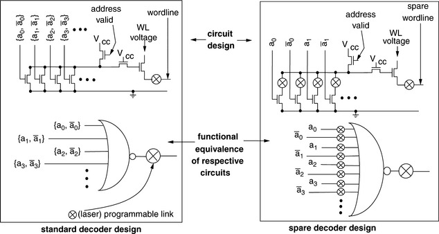
Figure 8.15 shows a set of standard and spare decoder designs that are used to drive rows of DRAM cells in some DRAM devices. In such a DRAM device, a standard decoder is attached to each of the 2n row of cells, and a spare decoder is attached to each of the spare rows. The figure shows that the standard decoder illustrated is functionally equivalent to an n-input NOR gate. In the standard decoder, each input of the functionally equivalent n-input NOR gate is connected to one bit in the n-bit address—either the inverted or the non-inverted signal line. Figure 8.15 shows that the spare decoder illustrated is functionally equivalent to a 2n-input NOR gate, and each bit in the n-bit address as well as the complement of each bit of the n-bit address is connected to the 2n inputs. In cases where a spare decoder is used, the input of the NOR gate is selectively disabled so that the remaining address signals match the address of the disabled standard decoder.
8.5.1 Row Decoder Replacement Example
Figure 8.16 illustrates the replacement of a standard decoder circuit with a spare decoder for a DRAM array with 16 standard rows and 2 spare rows. In Figure 8.16, the topmost decoder becomes active with the address of 0b1111, and each of the 16 standard decoders is connected to one of 16 standard rows. In the example illustrated in Figure 8.16, row 0b1010 is discovered to be defective, and the standard decoder for row 0b1010 is disconnected. Then, the inputs of a spare decoder are selectively disconnected, so the remaining inputs match the address of 0b1010. In this manner, the spare decoder and the row associated with it take over the storage responsibility for row 0b1010.

A second capability of the decoders shown in Figure 8.15, but not specifically illustrated in Figure 8.16, is the ability to replace a spare decoder with another spare decoder. In cases where the spare row connected to the spare decoder selected to replace row 0b1010 is itself defective, the DRAM device can still be salvaged by disconnecting the spare decoder at its output and programming yet another spare decoder for row 0b1010.
8.6 DRAM Device Control Logic
All DRAM devices contain some basic logic control circuitry to direct the movement of data onto, within, and off of the DRAM device. Essentially, some control logic must exist on DRAM devices that accepts externally asserted signal and control and then orchestrates appropriately timed sequences of internal control signals to direct the movement of data. As an example, the previous discussion on sense amplifier operations hinted to the complexity of the intricate timing sequence in the assertion of the wordline voltage followed by assertion of the SAN and SAP sense amplifier control signals followed yet again by the column-select signal. The sequence of timed control signals is generated by the control logic on DRAM devices.
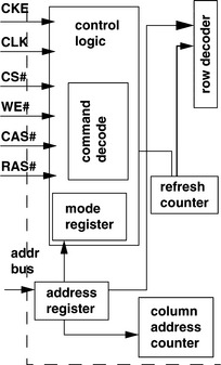
Figure 8.17 shows the control logic that generates and controls the timing and sequence of signals for the sensing and movement of data on the FPM DRAM device illustrated in Figure 8.1. The control logic on the FPM DRAM device asynchronously accepts external signal control and generates the sequence of internal control signals for the FPM DRAM device. The external interface to the control logic on the FPM DRAM device is simple and straightforward, consisting of essentially three signals: the row-address strobe (RAS), the column-address strobe (CAS), and the write enable (WE). The FPM DRAM device described in Figure 8.1 is a device with a 16-bit-wide data bus, and the use of separate CASL and CASH signals allows the DRAM device to control each half of the 16-bit-wide data bus separately.

In the FPM DRAM device, the control logic and external memory controller directly control the movement of data. Moreover, the controller to the FPM DRAM device interface is an asynchronous interface. In early generations of DRAM devices such as the FPM DRAM described here, the direct control of the internal circuitry of the DRAM device by the external memory controller meant that the DRAM device could not be well pipelined and new commands to the DRAM device could not be initiated until the previous command completed the movement of data. The movement of data was measured and reported by DRAM manufacturers in terms of nanoseconds. The asynchronous nature of the interface meant that system design engineers could implement a different memory controller that operated at different frequencies, and designers of the memory controller were solely responsible to ensure that the controller could correctly control different DRAM devices with subtle variations in timings from different DRAM manufacturers.
8.6.1 Synchronous vs. Non-Synchronous
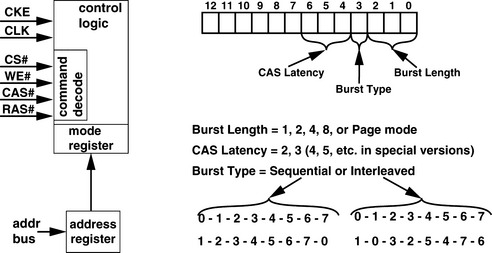
Modern DRAM devices such as synchronous DRAM (SDRAM), Direct Rambus DRAM (D-RDRAM), and dual data rate synchronous DRAM (DDR SDRAM) contain control logic that is more complex than the control logic contained in an FPM DRAM device. The inclusion of the clock signal into the device interface enables the design of programmable synchronous state machines as the control logic in modern DRAM devices. Figure 8.18 shows the control logic for an SDRAM device.
DRAM circuits are fundamentally analog circuits whose timing is asynchronous in nature. The steps that DRAM circuits take to store and retrieve data in capacitors through the sense amplifier have relatively long latency, and these latencies are naturally specified in terms of nanoseconds rather than numbers of cycles. Moreover, different DRAM designs and process variations from different DRAM manufacturers lead to different sets of timing parameters for each type and design of DRAM devices. The asynchronous nature and the variations of DRAM devices introduce design complexity to computing platforms that use DRAM devices as temporary memory storage. The solution deployed by the DRAM industry as a whole was the migration of DRAM devices to the synchronous interface.
The control logic for synchronous DRAM devices such as SDRAM and D-RDRAM differs from non-synchronous interface DRAM devices such as FPM and EDO in some significant ways. Aside from the trivial inclusion of the clock signal, one difference between control logic for synchronous and previous non-synchronous DRAM devices is that the synchronous DRAM devices can exhibit slight variations in behavior to a given command. The programmable variability for synchronous DRAM devices can be controlled by mode registers embedded as part of the control logic. For example, an SDRAM device can be programmed to return different lengths of data bursts and different data ordering for the column read command. A second difference between the control logic for synchronous DRAM devices and non-synchronous DRAM devices is that the synchronous control logic circuits have been designed to support pipelining naturally, and the ability to support pipelining greatly increases the sustainable bandwidth of the DRAM memory system. Non-synchronous DRAM devices such as EDO and BEDO DRAM can also support pipelining to some degree, but built-in assumptions that enable the limited degree of pipelining in non-synchronous DRAM devices, in turn, limit the frequency scalability of these devices.
8.6.2 Mode Register-Based Programmability
Modern DRAM devices are controlled by state machines whose behavior depends on the input values of the command signals as well as the values contained in the programmable mode register in the control logic. Figure 8.19 shows that in an SDRAM device, the mode register contains three fields: CAS latency, burst type, and burst length. Depending on the value of the CAS latency field in the mode register, the DRAM device returns data two or three cycles after the assertion of the column read command. The value of the burst type determines the ordering of how the SDRAM device returns data, and the burst length field determines the number of columns that an SDRAM device will return to the memory controller with a single column read command. SDRAM devices can be programmed to return 1, 2, 4, or 8 columns or an entire row. D-RDRAM devices and DDRx SDRAM devices contain more mode registers that control an ever larger set of programmable operations, including, but not limited to, different operating modes for power conservation, electrical termination calibration modes, self-test modes, and write recovery duration.
8.7 DRAM Device Configuration
DRAM devices are classified by the number of data bits in each device, and that number typically quadruples from generation to generation. For example, 64-Kbit DRAM devices were followed by 256-Kbit DRAM devices, and 256-Kbit devices were, in turn, followed by 1-Mbit DRAM devices. Recently, half- generation devices that simply double the number of data bits of previous-generation devices have been used to facilitate smoother transitions between different generations. As a result, 512-Mbit devices now exist alongside 256-Mbit and 1 Gbit devices.
In a given generation, a DRAM device may be configured with different data bus widths for use in different applications. Table 8.1 shows three different configurations of a 256-Mbit device. The table shows that a 256-Mbit SDRAM device may be configured with a 4-bit-wide data bus, an 8-bit-wide data bus, or a 16-bit-wide data bus. In the configuration with a 4-bit-wide data bus, an address provided to the SDRAM device to fetch a single column of data will receive 4 bits of data, and there are 64 million separately addressable locations in the device with the 4-bit data bus. The 256-Mbit SDRAM device with the 4-bit-wide data bus is thus referred to as the 64 Meg x4 device. Internally, the 64 Meg x4 device consists of 4 bits of data per column, 2048 columns of data per row, and 8192 rows per bank, and there are 4 banks in the device. Alternatively, a 256-Mbit SDRAM device with a 16-bit-wide data bus will have 16 bits of data per column, 512 columns per row, and 8192 rows per bank; there are 4 banks in the 16 Mbit, x16 device.

In a typical application, 4 16 Mbit, x16 devices can be connected in parallel to form a single rank of memory with a 64-bit-wide data bus and 128 MB of storage. Alternatively, 16 64 Mbit, x4 devices can be connected in parallel to form a single rank of memory with a 64-bit-wide data bus and 512 MB of storage.
8.7.1 Device Configuration Trade-offs
In the 256-Mbit SDRAM device, the size of the row does not change in different configurations, and the number of columns per row simply decreases with wider data busses specifying a larger number of bits per column. However, the constant row size between different configurations of DRAM devices within the same DRAM device generation is not a generalized trend that can be extended to different device generations. For example, Table 8.2 shows different configurations of a 1-Gbit DDR2 SDRAM device, where the number of bits per row differs between the x8 configuration and the x16 configuration.

In 1-Gbit DDR2 SDRAM devices, there are eight banks of DRAM arrays per device. In the x4 and x8 configuration of the 1-Gbit DDR2 SDRAM device, there are 16,384 rows per bank, and each row consists of 8192 bits. In the x16 configuration, there are 8192 rows, and each row consists of 16,384 bits. These different configurations lead to different numbers of bits per bitline, different numbers of bits per row activation, and different number of bits per column access. In turn, differences in the number of bits moved per command lead to different power consumption and performance characteristics for different configurations of the same device generation. For example, the 1-Gbit, x16 DDR2 SDRAM device is configured with 16,384 bits per row, and each time a row is activated, 16,384 DRAM cells are simultaneously discharged onto respective bitlines, sensed, amplified, and then restored. The larger row size means that a 1-Gbit, x16 DDR2 SDRAM device with 16,384 bits per row consumes significantly more current per row activation than the x4 and x8 configurations for the 1-Gbit DDR2 SDRAM device with 8192 bits per row. The differences in current consumption characteristics, in turn, lead to different values for tRRD and tFAW, timing parameters designed to limit peak power dissipation characteristics of DRAM devices.
8.8 Data I/O
8.8.1 Burst Lengths and Burst Ordering
In SDRAM and DDRx SDRAM devices, a column read command moves a variable number of columns. As illustrated in Section 8.6.2 on the programmable mode register, an SDRAM device can be programmed to return 1, 2, 4, or 8 columns of data as a single burst that takes 1, 2, 4, or 8 cycles to complete. In contrast, a D-RDRAM device returns a single column of data with an 8 beat12 burst. Figure 8.20 shows an 8 beat, 8 column read data burst from an SDRAM device and an 8 beat, single column read data burst from a D-RDRAM device. The distinction between the 8 column burst of an SDRAM device and the single column data burst of the D-RDRAM device is that each column of the SDRAM device is individually addressable, and given a column address in the middle of an 8 column burst, the SDRAM device will reorder the burst to provide the data of the requested address first. This capability is known as critical-word forwarding. For example, in an SDRAM device programmed to provide a burst of 8 columns, a column read command with a column address of 17 will result in the data burst of 8 columns of data with the address sequence of 17-18-19-20-21-22-23-16 or 17-16-19-18-21-20-23-22, depending on the burst type as defined in the programmable register. In contrast, each column of a D-RDRAM device consists of 128 bits of data, and each column access command moves 128 bits of data in a burst of 8 contiguous beats in strict burst ordering. An D-RDRAM device supports neither programmable burst lengths nor different burst ordering.

8.8.2 N-Bit Prefetch
In SDRAM devices, each time a column read command is issued, the control logic determines the duration and ordering of the data burst, and each column is moved separately from the sense amplifiers through the I/O latches to the external data bus. However, the separate control of each column limits the operating data rate of the DRAM device. As a result, in DDRx SDRAM devices, successively larger numbers of bits are moved in parallel from the sense amplifiers to the read latch, and the data is then pipelined through a multiplexor to the external data bus.
Figure 8.21 illustrates the data I/O structure of a DDR SDRAM device. The figure shows that given the width of the external data bus as N, 2N bits are moved from the sense amplifiers to the read latch, and the 2N bits are then pipelined through the multiplexors to the external data bus. In DDR2 SDRAM devices, the number of bits prefetched by the internal data bus is 4N. The N-bit prefetch strategy in DDRx SDRAM devices means that internal DRAM circuits can remain essentially unchanged between transitions from SDRAM to DDRx SDRAM, but the operating data rate of DDRx SDRAM devices can be increased to levels not possible with SDRAM devices. However, the downside of the N-bit prefetch architecture means that short column bursts are no longer possible. In DDR2 SDRAM devices, a minimum burst length of 4 columns of data is accessed per column read command. This trend is likely to continue in DDR3 and DDR4 SDRAM devices, dictating longer data bursts for each successive generations of higher data rate DRAM devices.

8.9 DRAM Device Packaging
One difference between DRAM and logic devices is that most DRAM devices are commodity items, whereas logic devices such as processors and application-specific integrated circuits (ASICs) are typically specialized devices that are not commodity items. The result of the commodity status is that, even more so than logic devices, DRAM devices are extraordinarily sensitive to cost. One area that reflects the cost sensitivity is the packaging technology utilized by DRAM devices. Table 8.3 shows the expected pin count and relative costs from the 2002 International Technology Roadmap for Semiconductors (ITRS) for high-performance logic devices as compared to memory devices. The table shows the trend that memory chips such as DRAM will continue to be manufactured with relatively lower cost packaging with lower pin count and lower cost per pin.

Figure 8.22 shows four different packages used in DRAM devices. DRAM devices were typically packaged in low pin count and low cost Dual In-line Packages (DIP) well into the late 1980s. Increases in DRAM device density and wider data paths have required the use of the larger and higher pin count Small Outline J-lead (SOJ) packages. DRAM devices then moved to the Thin, Small Outline Package (TSOP) in the late 1990s. As DRAM device data rates increase to multiple hundreds of megabits per second, Ball Grid Array (BGA) packages are needed to better control signal interconnects at the package level.

8.10 DRAM Process Technology and Process Scaling Considerations
The 1T1C cell structure places specialized demands on the access transistor and the storage capacitor. Specifically, the area occupied by the 1T1C DRAM cell structure must be small, leakage through the access transistor must be low, and the capacitance of the storages capacitor must be large. The data retention time and data integrity requirements provide the bounds for the design of a DRAM cell. Different DRAM devices can be designed to meet the demand of different markets. DRAM devices can be designed for high performance or low cost. DRAM-optimized process technologies can also be used to fabricate logic circuits, and logic-optimized process technologies can also be used to fabricate DRAM circuits. However, DRAM-optimized process technologies have diverged substantially from logic-optimized process technologies in recent years. Consequently, it has become less economically feasible to fabricate DRAM circuits in logic-optimized process technology, and logic circuits fabricated in DRAM-optimized process technology are much slower than similar circuits in a logic-optimized process technology. These trends have conspired to keep logic and DRAM circuits in separate devices manufactured in process technologies optimized for the respective device.
8.10.1 Cost Considerations
Historically, manufacturing cost considerations have dominated the design of standard, commodity DRAM devices. In the spring of 2003, a single 256-Mbit DRAM device, using roughly 45 mm2 of silicon die area on a 0.11-μm DRAM process, had a selling price of approximately $4 per chip. In contrast, a desktop Pentium 4 processor from Intel, using roughly 130 mm2 of die area on a 0.13-μm logic process, had a selling price that ranged from $80 to $600 in the comparable time-frame. Although the respective selling prices were due to the limited sources, the non-commodity nature of processors, and the pure commodity economics of DRAM devices, the disparity does illustrate the level of price competition in the commodity DRAM market. The result is that DRAM manufacturers are singularly focused on the low-cost aspect of DRAM devices. Any proposal to add additional functionalities must then be weighed against the increase in die cost and possible increases in the selling price.
8.10.2 DRAM- vs. Logic-Optimized Process Technology
One trend in semiconductor manufacturing is the inevitable march toward integration. As the semiconductor manufacturing industry dutifully fulfills Moore’s Law, each doubling of transistors allows design engineers to pack more logic circuitry or more DRAM storage cells onto a single piece of silicon. However, the semiconductor industry, in general, has thus far resisted the integration of DRAM and logic onto the same silicon device for various technical and economic reasons.
Figure 8.23 illustrates some technical issues that have prevented large-scale integration of logic circuitry with DRAM storage cells. Basically, logic-optimized process technologies have been designed for transistor performance, while DRAM-optimized process technologies have been designed for low cost, error tolerance, and leakage resistance. Figure 8.23 shows a typical logic-based process with seven or more layers of copper interconnects, while a typical DRAM-optimized process has only two layers of aluminum interconnects along with perhaps an additional layer of tungsten for local interconnects. Moreover, a logic-optimized process typically uses low K material for the inter-layer dielectric, while the DRAM-optimized process uses the venerable SiO2. Figure 8.23 also shows that a DRAM-optimized process would use four or more layers of polysilicon to form the structures of a stacked capacitor (for those DRAM devices that use the stacked capacitor structure), while the logic-optimized process merely uses two or three layers of polysilicon for local interconnects. Also, transistors in a logic-optimized process are typically tuned for high performance, while transistors in a DRAM-optimized process are tuned singularly for low-leakage characteristics. Finally, even the substrates of the respectively optimized process technologies are diverging as logic-optimized process technologies move to depleted substrates and DRAM-optimized process technologies largely stays with bulk silicon.

The respective specializations of the differently optimized process technologies have largely succeeded in preventing widespread integration of logic circuitry with DRAM storage cells. The use of a DRAM-optimized process as the basis of integrating logic circuits and DRAM storage cells leads to slow transistors with low-drive currents connected to a few layers of metal interconnects and a relatively high K SiO2 inter-layer dielectric. That is, logic circuits implemented on a DRAM-optimized process would be substantially larger as well as slower than comparable circuits on a similar generation logic-optimized process. Conversely, the use of a higher cost logic-optimized process as the basis of integrating logic circuits and DRAM storage cells leads to high-performance but leaky transistors coupled with DRAM cells with relatively lower capacitance, necessitating large DRAM cell structures and high refresh rates.
In recent years, new hybrid process technologies have emerged to solve various technical issues involving the integration of logic circuits and DRAM storage cells. Typically, the hybrid process starts with the foundation of a logic-optimized process and then additional layers are added to the process to create high-capacitance DRAM storage cells. Also, different types of transistors are made available for use as low-leakage access transistors as well as high-drive current high-performance logic transistors. However, hybrid process technology then becomes more complex than a logic-optimized process. As a result, hybrid process technologies that enable seamless integration of logic and DRAM devices are typically more expensive, and their use has thus far been limited to specialty niches that require high-performance processors and high-performance and yet small DRAM memory systems that are limited by the die size of a single logic device. Typically, the application has been limited to high-performance System-on-Chip (SOC) devices.
1RAS is known as both row-address strobe (more common) or as row-access strobe. The author prefers “access” because of the way the DRAM access protocol has morphed from more of a signal-based interface to a command-based interface. Both “address” and “access” are commonly accepted usage for “A” in both RAS and CAs.
2The FPM DRAM device illustrated in Figure 8.1 does allow each 8-bit half of the 16-bit column to be accessed independently through the use of separate column-access strobe high (CASH) and column-access strobe low (CASL) signals. However, since the data bus is 16 bits wide, a column of data in this device is 16 bits rather than 8 bits. Equivalently, modern DRAM devices make use of data mask signals to enable partial data write operations within a single column. Some other DRAM devices such as XDR devices make use of sophisticated command encoding to control sub-column read and write operations.
3The first commercial DRAM device, Intel’s 1103 DRAM device, utilized a 3T1C cell structure.
4The variable leakage problem is a well-known and troublesome phenomenon for DRAM manufacturers that leads to variable retention times (VRTs) in DRAM cells.
5In some modern DRAM devices that use trench capacitors, the depth-to-width aspect ratio of the trench cell exceeds 50:1.
6The integration of DRAM cells with the logic circuit on the same process technology is non-trivial. Please see the continuing discussion in Section 8.10.
7Bitlines are also known as digitlines.
8Currently, most manufacturers utilize DRAM cells that occupy an area of 8 F2, and the International Technology Roadmap for Semiconductors (ITRS) predicts that DRAM manufacturers will begin transition to new DRAM cell structures that are only 6 F2 in 2008. However, Micron announced in 2004 that it had succeeded in the development of a Metal-Insulator-Metal (MIM) capacitor that occupies an area of 6 F2 and began shipping products based on this structure in 2004 and 2005.
9In modern DRAM devices, the timing and shape of the SAN and SAP control signals are of great importance in defining the accuracy and latency of the sensing operation. However, for the sake of simplicity, the timing and shape of these important signals are assumed to be optimally generated by the control logic herein.
10Some DRAM devices, such as Direct RDRAM devices, have write buffers. Data is not driven directly into the DRAM array by the data I/O circuitry in that case, but the write mechanism into the DRAM array remains the same when the write buffer commits the data into the DRAM array prior to a precharge operation that closes the page.
11The row cycle times of most DRAM devices are write-cycle limited. That is, the row cycle times of these DRAM devices are defined so that a single, minimal burst length column write command can be issued to a given row, between an activation command and a precharge command to the same row.
12In DDRx and D-RDRAM devices, 2 beats of data are transferred per clock cycle.