
Performance Testing
Performance testing is an important part of the design and development of a new disk drive. This chapter is devoted to the discussion of testing and measuring the performance of a disk drive. Because of the complexity of the entire disk drive and the sensitivity of its behavior to different environments and access sequences, precise performance information can only be obtained by running tests on the actual drive. Simulation may be able to predict the mechanical timing quite accurately. Exact prediction of the cache’s effect is harder, as the amount of data that gets prefetched is sensitive to how accurately the time available for prefetching is simulated. This available time for prefetching depends not only on the drive’s own overhead, but also on activities that go on in the host in between I/Os.
Benchmarks are standard test programs which allow a user to test different devices in an identical manner such that the devices’ performance can be compared on an equal footing. They play an important role in the world of disk drives as buyers, large and small, do pay attention to benchmark results when making their purchase decisions. This chapter will discuss some of the ins and outs of benchmark programs.
Not only can testing the timing of execution of a particular I/O command reveal the performance characteristics of a drive, it can also be used to determine many of the implementation details of a disk drive. By applying specially designed I/O test patterns to a drive and measuring the response times of those commands, it is possible to derive certain drive parameters such as its geometry (data layout scheme) and seek profile [Worthington et al. 1995]. This technique and some of these test patterns will be discussed in this chapter.
23.1 Test and Measurement
As discussed in Chapter 16, Section 16.3, the performance of a drive is measured in terms of either throughput or response time. Throughput can either be expressed as the number of I/Os per second (IOPS) completed, or as number of megabytes per second (MB/s) transferred. The two are related by the block sizes of the I/Os. For example, 200 IOPS with a single block size of 4 KB translates to 0.8 MB/s. If half of the blocks are of size 4 KB and the other half are of size 64 KB, then the 200 IOPS translates to 6.8 MB/s. Throughput implies measuring the total elapsed time for completing a large number of I/Os and then dividing either the number of I/Os or the number of bytes by that total time. Response time, on the other hand, is measured for an individual I/O. However, it is much more typical to discuss performance in terms of average response time, in which case the response times of many I/Os over a period of time are added up and divided by the number of I/Os.
Three components are needed for testing the performance of a disk drive. The first component is some mechanism, call it a test initiator, for generating and issuing the I/O commands for the drive to execute as the test sequence for performance measurement. The second component is some means for monitoring and measuring. The third component is, of course, the disk drive itself.
23.1.1 Test Initiator
A dedicated piece of hardware, one which provides a standard interface to which a disk drive can be attached, is certainly one option for a test initiator. A simpler, and perhaps more flexible, option is to use a general-purpose personal computer or workstation. One or more types of standard interfaces are usually available in such a machine. Add-on interface cards for any interface are also available. One can write software that issues test I/O commands to the drive directly. Alternatively, one can issue high-level read and write commands to the system’s device driver. A device driver is a piece of operating software that provides the service of performing high-level read and write commands by handling all the necessary standard interface handshakes. By using the service of the device driver, the test initiator creator does not need to know the intricate details of talking to a disk drive directly, though, of course, knowledge of the device driver interface is required.
Test Sequence Characteristics
The sequence of I/O commands issued by a test initiator to a disk drive is characterized by the following elements:
Command type Read and write are the most commonly used commands, but other commands such as flush and reset may also be issued by the test initiator. A sequence may be composed of a certain percentage of reads and a certain percentage of writes, or it may be composed of all reads or all writes.
LBA distribution The addresses may be sequential from one command to the next, localized to a small section of the disk’s address space, composed of multiple sequential streams interleaved, or perhaps completely random.
Block size The request size can be a fixed number of sectors, all small blocks, all large blocks, a mixture with some predefined distribution (e.g., 70% 4 KB and 30% 64 KB), or some random mixture of block sizes.
Command arrival time The test initiator has control of the inter-arrival time between issuing commands. Thus, it can determine both the average command arrival rate and the distribution.
Queue depth The test initiator can also control how many I/Os to queue up in the disk drive at any point in time. For example, it can keep the queue at its maximum at all times, or it can throttle the number of commands sent to the drive in order to achieve a certain response time (maximum or average).
Methods of Test Generation
There are three main ways of generating the test I/Os that are to be sent to the disk drive:
Internally created The I/Os are created by the test initiator according to certain characteristics. The characteristics are usually specifiable by the user. For instance, a user may ask for testing how a disk drive performs doing random reads of 4 KB blocks with a queue depth of 16 within an address range of 100 MB between LBAs 600,000 and 800,000. More commonly, the user would ask for a battery of such tests with a range for each characteristic, e.g., block sizes of 1, 2, 4, 8, 16, 32, 64, and 128 KB; queue depths of 1, 2, 4, 8, 16, and 32; for read and for write commands; etc. The test initiator uses a random number generator to create I/O requests in accordance with the specified characteristics.
Predefined sequence The test initiator reads an input file which contains a predefined I/O sequence, and issues those I/Os to the disk drive in exactly the same order and with the same inter-arrival time between commands as recorded in the file. The I/O sequence can be manually created by the user to very specifically probe for how a disk drive performs or behaves with that particular sequence. This is how some drive parameters can be extracted, as will be discussed later. Alternatively, the sequence can be a recorded trace obtained by monitoring the I/Os sent to a disk drive while performing certain activities. In this case, the test initiator is simply playing back the previously recorded trace. Because exactly the same I/O sequence is sent to the drive every time, analysis of the results from this method of testing can be very precise. For instance, the change in performance due to an alteration in the disk drive can be accurately measured. One can also use this method to compare the performances of two different drives fairly, since the drives will be seeing exactly the same sequence of I/O requests. Some benchmark programs use this method of testing.
Application based A third way of generating the I/O test sequence is for the test initiator to invoke application programs to perform certain tasks. The objective is to see how well a disk drive performs in the execution of such applications. A predefined test script of what application functions to call and what commands to issue is used. Unlike the playback of predefined I/O commands, real files need to be set up first for the application programs to work on. This method of testing at a higher level is also used by some benchmark programs. The sequence of I/O commands that actually gets sent to the disk drive depends on the operating systems, where the test files are created, how much system memory there is in the host system, and a host of other factors. Therefore, it is likely that there is variation in the I/O sequence from system to system and even from run to run.
23.1.2 Monitoring and Measuring
Whether determining throughput or response time, testing the performance of a drive requires timing the elapse time between one event and another event. The first event is usually the start of an I/O request, and the second event is the end of the same or some other I/O request. There are three points in the system where monitoring and clocking of the events can be done, as shown in Figure 23.1.
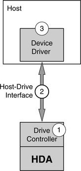
FIGURE 23.1 Monitor points: 1. inside the disk drive; 2. at the interface; 3. at the device driver level.
Inside the disk drive By instrumenting the firmware of the drive controller, the beginning and the end of almost any drive activity can be very precisely monitored and timed. Clearly, only the drive maker will have this capability. Some drive activities may also be measured by probing with an oscilloscope. However, very good knowledge of the drive’s circuit will be needed to know what points to probe. When making measurements at this low level, it is possible to measure just the execution time of an I/O and exclude the overhead of the drive controller. Thus, one can measure precisely the time to fetch data out of the cache if it is a cache hit or the seek, latency, and media transfer time if disk access is required. Of course, controller overhead can be measured here also. Instrumentation of the firmware adds code to perform the monitoring function while executing an I/O request. Thus, this method necessarily perturbs the actual execution timing of running a sequence of I/Os.
At the interface Bus monitors are available for all standard interfaces. Such hardware usually consists of a pod containing the monitoring circuits and either a dedicated system or a general-purpose computer which runs the control software. The pod intercepts and passes on all the signals that go between the drive and the host. The cable coming out of the drive plugs into one end of the pod, while the cable coming out of the host plugs into another end. No internal knowledge or access of the drive is required for doing measurements at this level. A bus monitor will work with any drive from any manufacturer. However, it does require understanding of the interface standard to use and interpret the results of this tool. Quite accurate timing, with sub-microsecond accuracy, can be measured. Writing the command register by the host in ATA or sending the CDB in SCSI marks the start of an I/O request. The drive responding with completion status marks the end of a command. The elapsed time between those two events measures the sum of the I/O execution time of the drive and the overhead incurred by the drive controller. Because this method is non-invasive, the actual timing of running a sequence of I/Os is not perturbed.
At or above the device driver By instrumenting the device driver or adding a monitor layer just above the device driver, the execution time of an I/O as seen by the device driver or the user of the device driver can be measured. This method is simple because knowledge of the internal disk drive or the interface is not required. The timing accuracy is dependent on the resolution of the system clock readable by the software. Also, the timing of an I/O will necessarily include the overhead of the device driver, obscuring the actual execution time of the disk drive. Finally, the addition of monitor code adds extra overhead which will perturb the actual execution timing of running a sequence of I/Os.
23.1.3 The Test Drive
There are a few things that one should be aware of regarding the drive whose performance is to be measured.
Drive-to-drive variation Even for drives of the same model and capacity, it is likely that there will be some degree of variation from drive to drive. Part of this is simply due to the nature of electro-mechanical devices, where some variation is to be expected. Other factors may also contribute. For example, the data layouts and address mappings of two same model drives may be different because of adaptive formatting (discussed in Chapter 25, Section 25.5). Therefore, ideally, several drives should be tested in order to get the average performance for a particular model of disk drive.
Run-to-run variation For a given test drive, there is also some variation likely from one test run to the next. Again, this is simply the nature of the electro-mechanical device. Certain things such as media data rate will be quite stable and show no variation. Other things such as I/O times that require seeking will exhibit some variation. Therefore, depending on the nature of the test being conducted, some tests may need to be repeated a number of times to get an average measurement.
Mounting Seek time is susceptible to vibration in the disk drive, and vibration is dependent on how the drive is mounted. There are two acceptable ways to mount a drive for testing its performance. One method is to mount the test drive to a heavy metal block resting on a solid surface so as to minimize the amount of vibration. This measures the performance of the drive under an ideal condition. A second method is to test the drive mounted in the actual system where it is intended to be used. This measures the real-life performance that the drive can be expected to produce in its target system.
Write tests For test sequences that are generated below the operating system’s file system, such as randomly generated I/Os or a replay of some predefined sequence, writes can go to any location in the disk drive. This means that previously recorded data on the test drive can be overwritten without any warning. One should be aware of this consequence before doing any testing on a disk drive.
23.2 Basic Tests
The raw performance of a disk drive can be measured using a number of basic tests. The performance characteristics that can be measured include data rate (bandwidth), IOPS (throughput), and response time, for reads as well as for writes. The basic tests are therefore quite simple and straightforward.
A user can fairly easily create his own test initiator for performing basic tests. However, there are a number of such test programs available for free that can be downloaded from the Internet, and so, unless one has a need to very precisely control the testing in a particular way, there is little reason to build one from scratch. Most of these tools perform similar tests, differing only in the user interface.
There is no standard definition of what a set of basic tests should consist of. A few common ones are selected to be discussed here.
23.2.1 Media Data Rate
Most programs test the data rate of a drive by issuing a long sequence of sequential reads of a large block size. Since this results in reading many tracks of data, what gets measured is the drive’s sustained data rate, as discussed in Chapter 18, Section 18.8. When measurement is taken at the host level, the results may be somewhat affected by the overhead for handling each command. However, by using a large block size to reduce the frequency of such overheads, the combined effect of a faster interface data rate and the action of lookahead prefetch will be able to hide these overheads so that the measured results are truly the drive’s sustained data rate.
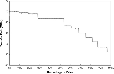
Because of zoned-bit recording, the measured data rate of a drive depends on where on the disk the test is run. If the entire disk is tested, then a picture of the test drive’s zones is revealed. Figure 23.2 shows an example of such a read test result for an actual disk drive. Here, the average data rates measured for each 0.1% of the drive’s total capacity are plotted. For this drive, 11 distinct data rates and zones are clearly visible. A similar write test can be performed for measuring the media data rate. Write results typically exhibit more noise due to some occasional write-inhibits, as writes require more stringent conditions to proceed than reads. A write-inhibit would cause the drive to take one or more revolutions to retry the write. Thus, the test result for the write data rate usually shows up slightly lower than the read data rate for the same drive, even though in reality the raw media data rate is the same for both reads and writes.
23.2.2 Disk Buffer Data Rate
Though the speed of the drive’s DRAM buffer is high, its actual realizable data rate as observed by the host is limited by both the speed of the drive-host interface and the overhead of the drive in doing data transfer. To test this data rate, the test pattern would simply be reading the same block of data repeatedly many times. Since the same block of data is read, only the cache memory is involved. If a large block size is chosen, then the effect of command overhead is minimized, just as in the media data rate test discussed previously. Smaller block sizes can be chosen to observe the impact of command overhead.
23.2.3 Sequential Performance
The media data rate test is one special case of sequential performance measurement. In many actual applications, smaller block sizes are used for data requests. With small block sizes, the effect of command overhead in lowering the achievable data rate becomes visible. Therefore, a standard sequential performance test would measure the throughput at various block sizes. Figure 23.3 shows an example of sequential read measurement results of another actual drive. The throughput expressed as IOPS is also plotted. Note that as the block size increases, the data rate attained also increases as the amount of command overhead per byte becomes less. By the time a block size of 16 KB is reached, all overheads can be overlapped with the media data transfer time, and the sustained data rate is being measured.

Because lookahead prefetch, if properly implemented, can take care of streaming sequential read data from the media to the buffer without interruption, command queueing has almost no effect for sequential reads. Usually, only a very slight increase in throughput can be observed for small block sizes when going from no queueing to a queue depth of 2.
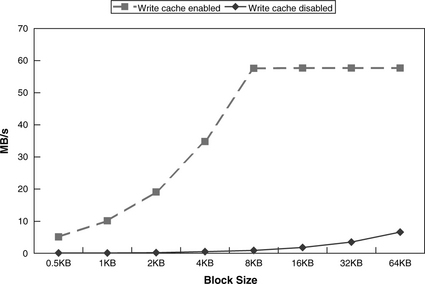
A similar situation occurs for sequential writes if write caching is enabled. The interface data rate is fast enough to fill the buffer with data for streaming to the media without any hiccup. However, if write caching is not enabled, each write command will take one disk revolution to complete, resulting in very low throughput, as shown in Figure 23.4. Using command queueing with a sizable queue depth is needed to avoid having to take one revolution to do each write command when write caching is not enabled.
23.2.4 Random Performance
Sequential performance tests measure the media data rate of the drive, its command handling overhead, and the effectiveness of its cache in lookahead prefetch. As such, the performance of the mechanical components does not get exercised. On the other hand, random accesses require seeks and rotational latencies. Thus, the purpose of random performance tests is to measure the mechanical speed of the drive. It is conducted by generating random addresses within a specified test range, oftentimes the whole drive, to do reads and writes. While it certainly is possible to measure and report random performance in a fashion similar to that shown in Figure 23.3 for sequential performance, the use of larger block sizes is a distraction as the longer data transfer time only serves to dilute any differences in mechanical times. It is more informative to measure random performance using the smallest possible block size.
An alternative way to report random performance is to tabulate and plot a histogram of the fraction of I/Os that is completed for each incremental unit of time. Figure 23.5 illustrates such a result for an actual 4200 rpm drive, with a bucket size of 1 ms increments. The test result for single sector reads is shown in Figure 23.5(a). The average response time is calculated to be 18.46 ms, which should be the sum of average seek time, average latency time (one-half revolution time), all command overheads, and a negligible data transfer time. Since the average latency for a 4200-rpm drive is 7.1 ms, it can be deduced that the average read seek time for this drive is in the neighborhood of 10 ms. There is a bell-shaped distribution around this average read I/O time. The near tail at around 2 ms represents approximately no seek and very little latency and so is essentially the sum of all the overheads.
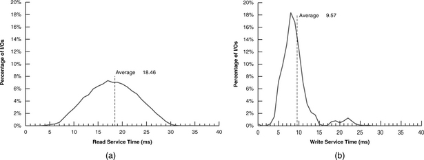
FIGURE 23.5 Histogram of the I/O completion time for single sector random accesses. The drive is 4500 rpm with write cache enabled: (a) random reads and (b) random writes.
The far tail, at around 31 ms, represents approximately full stroke seek and maximum latency (one revolution). The test result for single sector writes of the same drive is shown in Figure 23.4(b). It looks very different from the curve for reads because of write caching. While for most drives the shapes of the read curves will be similar to the one shown here, the write curves will likely have different shapes since they depend on the write caching algorithm implemented, and different drives are likely to have somewhat different algorithms. For instance, the number of cached writes allowed to be outstanding and the timing of when to do destaging are design parameters that vary from drive to drive. If write caching is disabled, then the write curve will look similar to the read curve, with the average I/O time and the curve shifted slightly to the right due to the higher settling time for write seeks compared to read seeks.
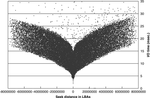
Another informative way to display the result of a random access test is to plot the I/O completion time for each command against the seek distance for that command. To simplify things, the seek distance can be expressed in number of LBAs, i.e., take the LBA of the previous command and subtract that from the LBA of the current command. An example of such a plot for 32,000 random reads is shown in Figure 23.6, which is for an actual 40-GB, 4200-rpm mobile drive. Some refer to such a plot as a “whale tail,” while others call it a “moustache,” for obvious reasons. The bottom outline of the “tail” approximately represents the seek curve of the drive, since those are the I/Os that can be completed immediately after arrival on the target track without any latency. For this drive, the forward seek (toward the ID) time is slightly longer than the backward seek (toward the OD) time. The vertical thickness of the tail represents the revolution time of the drive, which is 14.3 ms for a 4200-rpm drive. There are a few sprinkles of points above the top outline of the tail. These are reads that need to take an extra revolution or two for retries (see Chapter 18, Section 18.9).
23.2.5 Command Reordering Performance
Command reordering, as discussed in Chapter 21, Section 21.2, can significantly boost the performance of a disk drive. Since the name of the game is to reduce the mechanical portion of an I/O’s execution time, especially in handling random accesses, it would make sense to test for a drive’s command reordering effectiveness using the smallest block size, just as in the case for random access performance measurement. The most straightforward way to conduct a performance measurement test of command reordering is to issue random single sector accesses to a drive over a reasonable period of time at various queue depths.
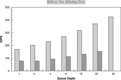
The average throughput for each queue depth can then be recorded and plotted. The access type can be all reads, all writes, or a certain percentage of each that is of interest to the tester. Throughput is a better metric than response time in this case because response time (lower is better) will go up with queue depth (a command needs to wait longer when there are more other commands in the queue), even though command reordering effectiveness usually improves with higher queue depths. Figure 23.7 plots the test results of two different drives: a 15000-rpm SCSI server drive with an average seek time of around 3.3 ms and a 7200-rpm SATA desktop drive with an average seek time of about 8.2 ms. While the throughputs for these two drives both improve as command queue depth is increased, the far superior mechanical properties of the high-end server drive are quite evident.
23.3 Benchmark Tests
The purpose of benchmarks is for users and developers to have a means to measure and make meaningful apple-to-apple performance comparison, whether between two products from two different manufacturers, from generation to generation of a product by the same manufacturer, or from one design/implementation revision to the next during product development. A benchmark is a test, or a set of tests, which measures performance, and it must be generally available to the public. Benchmark tests for storage have been around for many years; some have come and gone, while others evolve. Some storage benchmarks are targeted for storage systems with multiple drives, and some are designed for individual disk drives. Most disk drive benchmarks can also be tested on a logical volume of a storage system.
Some drive benchmarks are application based, constructed to determine how well a drive does in running the applications of interest. The Disk WinMark tests of WinBenchTM99,1 which has been one of the popular disk benchmarks in the past few years, is one such example. It was created by surveying the user community to gather a collection of the most commonly used application programs in a PC. Other benchmark programs are replays of predefined sequences, although such sequences can be from tracing the execution of application programs and so, in a sense, are application based rather than artificially created. PCMarkTM05,2 which is now popular as a disk benchmark, is one such example.
There is another group of special tests that are also designed to measure drive performances. These are the proprietary tests that large original equipment manufacturers (OEMs) have created for their own internal use in evaluating disk drives that would go into their products. While these tests serve the same purpose as benchmarks, technically they cannot be called benchmarks because they are not available to the general public. Nonetheless, for all intents and purposes, these proprietary tests can be treated the same as benchmarks, and the discussion in the following section applies to them equally.
23.3.1 Guidelines for Benchmarking
There are a few points that one should be aware of when benchmarking disk drives. Understanding and following these guidelines are necessary for obtaining correct benchmark measurements. Otherwise, misleading results might be obtained, leading to incorrect conclusions.
Test System
It matters what system is being used to measure the benchmark performance score of a disk drive. Because a benchmark does its test monitoring and timing high up in the system level, it is unavoidable that measurements include at least some amount of system time. Thus, a benchmark, in reality, measures the combined performance of the host system, the interface, and the disk drive. The percentage of a benchmark’s score that is actually attributed to the disk drive’s performance depends on which benchmark is used. A good disk benchmark should have a high percentage, minimizing, though not eliminating, the influence of the host system and interface.
Various components of the system all contribute to affecting a benchmark’s result. The speed of the CPU has the obvious effect on the timing on the system side. The data rate of the interface affects the data transfer time. Additionally, for application-based benchmarks, the amount of memory in the system determines how much data would be cached in the host, thus affecting the number of I/Os that actually get sent down to the disk drive. The operating system also plays a visible role. The file system determines the size of allocation units and where to place the test data. A journaling file system issues additional I/Os for logging the journal compared to a non-journaling file system. Finally, how I/Os are being sent to the drive can be influenced by the device driver used.
If a report says that drive A has a benchmark score of 1000, and somebody measures drive B in his system to have a score of 900 using the same benchmark, what conclusion can be drawn? Nothing. The two systems may be very different, and so it is possible that drive B is actually a faster drive despite the lower score. Therefore, to obtain meaningful comparison, benchmarking should be performed using the same system or two identically configured systems.
Ideal Setup
An ideal way to set up for benchmarking is to have a disk drive in the system already loaded with the operating system and all the benchmark programs of interest, and the drive to be tested is simply attached to this system as another disk. One obvious advantage is avoiding having to spend the time to install the operation system and load the benchmark programs onto the test drive. Thus, once the system is set up, many different drives can quickly be tested this way since there is no preparation work required for the disk drive.
A second advantage is that such a setup allows a completely blank disk to be tested. This allows all disks to be tested in exactly the same condition. It also enables the same disk to be tested repeatedly in exactly the same condition. If, on the other hand, the test disk must have an operating system and other software loaded into it first, then the test result can potentially be affected by how things are loaded into the drive.
Multiple Runs
As discussed earlier, a disk drive is an electromechanical device, and so most performance measurements will likely vary somewhat from run to run. Hence, a benchmark test should be repeated a few times to obtain an average score.
Between one run to the next, the drive should be either reformatted to restore it to a blank disk if the drive is tested as a separate drive in an ideal setup or defragged to remove any fragmentation if it also holds the operating system and other software. Certain application-based benchmarks may generate temporary files, thus creating some fragmentation at the conclusion of the tests. Such fragmentations will accumulate if not cleaned up after each run and degrade user performance over time. Finally, the drive should then be power-cycled to set it back to its initial state, such as an empty cache.
23.4 Drive Parameters Tests
When specially designed test patterns are applied to a disk drive and the response times of each command are monitored and measured, some of the parameters of a disk drive can be deduced. The media data rate test, as illustrated in Figure 23.2, can be considered to be one such test which measures the number of recording zones in a drive. The whale tail plot for random accesses, as illustrated by Figure 23.6, may also be considered as another example in which a drive’s seek profile and rotational time can be measured, albeit not very accurately. In this section, a couple of examples of special test patterns for precisely determining several important parameters of a drive are discussed.
23.4.1 Geometry and More
The geometry of a drive is described by such things as the number of sectors per track, how the tracks are laid out (number of tracks per cylinder if cylinder mode is used, or serpentine formatting), and the number of recording zones. More than one method involving distinctly different test patterns can be used to extract such drive parameters [Ng 2001a,b]. One such method will be discussed in this section. The overall approach is the same for all methods. The first step is to identify the track boundaries. Then, the number of LBAs between two identified track boundaries is used to establish the number of sectors per track. The skew at each track boundary is next derived from the measured data. For most drives the cylinder skew is bigger than a track skew. By comparing the sizes of the skews for a large enough group of track boundaries, the cylinder boundaries can be identified and the number of heads per cylinder deduced. This would be the scenario for cylinder mode formatting. For a drive with serpentine formatting, there will be many (tens or even hundreds) same size skews followed by a different size skew. Finally, if the process is applied to the whole drive, then details of every zone can be exposed.
The following describes one test method by way of an example of a highly simplified hypothetical disk drive using the traditional cylinder formatting. Read commands will be used in the discussion. Either reads or writes can be used with the test pattern, but reads would be preferable since the content of the drive would then not be destroyed in the testing process. Caching will need to be turned off for the test to force the drive to access the media for each command.
A Test Method
The test pattern for this method is very simple. A single sector read command is issued for a range of sequential addresses. The address range is for the area of the disk drive that is to be tested. The size of the range should be at least two or three times the estimated size of a cylinder of the drive and can be as large as the complete address range of the whole drive. The commands are issued one at a time synchronously, with the next command issued by the host as soon as the previous command is completed. The time of completion of each command, which can be monitored at any of the levels described in Section 23.1.2, is recorded. The elapsed time between the completion times of every pair of consecutive commands is calculated and plotted. This elapsed time, while consisting of the drive overhead, seek time (if any), rotational latency time, data transfer time, as well as the host system’s processing time, is actually dictated by the physical relationship between the two addresses. For example, if the two addresses are physically contiguous on the disk, then the delta time is one revolution plus the rotation time of one sector. If one address is the last logical sector of a track and the other address is the first logical sector of the next track, then the delta time is most likely one revolution plus the track/cylinder skew plus the rotation time of one sector.
Figure 23.8 shows the results for reading LBAs 0–99 of the hypothetical example disk drive. It can be seen here that most of the delta times are 10.5 ms. These are the times for reading the next physical sector on the same track, which is naturally the most frequent. Hence, each represents one revolution plus a sector time. It can be observed that the delta times to read LBAs 20, 40, 60, and 80 are longer than the typical 10.5 ms. It can be assumed that these sectors are the first logical sectors after a track boundary, and hence, the delta time includes a skew time in addition to the revolution and one sector time. Since there are 20 sectors between each of these LBAs, it can be deduced that there are 20 sectors per track for this disk drive. Furthermore, the 13.5-ms delta times at LBAs 40 and 80 are larger than the 12.5-ms delta times at LBAs 20 and 60. It can be concluded that this drive exhibits the typical characteristics of a traditional cylinder mode format. Whereas LBAs 20 and 60 are after a head switch, with a track skew of 12.5–10.5 = 2.0 ms, LBAs 40 and 80 are after a cylinder switch, with a cylinder skew of 13.5–10.5 = 3.0 ms. Since there is only one head switch between cylinder switches, it can be deduced that there are only two tracks per cylinder. Hence, this must be a single platter disk with two heads.

This example illustrates a simple idealized drive. It shows a drive with the same number of sectors per track. In real drives, some tracks may have fewer sectors than the majority of tracks. The missing sectors are either reserved for sparing or defective sectors that have been mapped out. If a drive uses a cylinder skew which is equal to the track skew, then this test method will not be able to determine the number of tracks per cylinder. However, the number of heads in a drive is usually given in the drive’s spec sheet.
If a track has N sectors, then the rotation time of one sector is simply 1/N of a revolution. In other words,
For this example, N = 20, and the revolution time plus sector time is 10.5 ms. Using these numbers Equation 23.1 can be solved to give a revolution time of 10 ms. This translates to a rotational speed of 6000 rpm for the hypothetical drive of this example.
Finally, by running the test pattern of this method from LBA 0 all the way to the last LBA of the drive, the precise zoning information of the entire drive can be revealed. Continuing with the example, Figure 23.9 illustrates the results of doing so for the hypothetical drive. Three zones are clearly visible. The first zone, whose sectors per track, tracks per cylinder, and skews have already been analyzed, contains three cylinders with the address range of LBAs 0–119. The second zone, from LBAs 120–179, has 15 sectors per track and 2 cylinders. The third zone, with the address range LBAs 180–239, has 3 cylinders and 10 sectors per track.

FIGURE 23.9 The result of the geometry test for the entire hypothetical drive. Three zones are clearly visible.
Roughly one revolution is needed to read one sector; hence, for a 400-GB disk with 7200 rpm, it would take over 1800 hours to complete. This is clearly not practical. The alternative is to apply this test method to various portions of the disk to sample the geometry at those locations. If the precise zone boundaries need to be determined, a binary hunt method can be applied to zero in on those boundaries.
23.4.2 Seek Time
While the random access test result presented in a whale tail plot format gives a rough profile of a drive’s seek characteristics, a specialized test procedure tailored to measure seek time will provide more precise information. One such method is described here.
The first step is to apply the test method discussed in the previous section to extract the geometry information of the drive. To test for the seek time between two cylinders of interest, select any sector in the starting cylinder. This will be the anchor sector for the test. Next, select a track in the ending cylinder to be the target track. The test pattern is to alternate reading the anchor sector and a sector from the target track. For example, if the target track has LBAs 10000–10999, and the anchor sector is selected to be LBA 0, then the test pattern is to read LBA 0, 10000, 0, 10001, 0, 10002, …, 0, 10998, 0, and 10999. The purpose of reading the anchor sector is to reorient the head of the disk to a fixed starting position. As in the geometry test, the delta times between the completion of commands are recorded and plotted, except that here only the delta times going from the anchor sector to the target track are plotted. Each of these delta times represents the sum of the seek time, the rotational latency time, all command overheads, and the data transfer time of one sector.
Analysis of the test result is explained by way of another highly simplified hypothetical drive. Figure 23.10(a) shows the piece-wise linear approximation of the seek profile of the hypothetical drive. At a seek distance of 3000 cylinders, the seek time is 10 ms. Let’s assume that we want to measure the seek time from cylinder 0 to cylinder 3000. LBA 0 is as good as any to be selected as the anchor sector. For this hypothetical drive, there are 100 sectors per track at cylinder 3000. Figure 23.10(b) plots the test result, showing the delta times between completion of an anchor read and read completion for each of the sectors in the target track. The maximum delta time, as marked with B, is for the sector which just misses the head when the head arrives on the target track and has to wait for basically one full revolution. The minimum delta time, as marked with A, is for the first sector that the head is able to read after it has arrived on track and settled. Thus, its rotational latency, which is half a sector’s time on average, is negligible. Therefore, the minimum delta time is essentially the sum of the seek time, all command overheads, and one sector rotation time (0.1 ms in this hypothetical example, but typically much smaller for a real disk with many times more sectors per track). So, this test method yields a result of 10.5 ms for a 3000-cylinder seek, including overheads. If command overheads can somehow be measured and subtracted from the result of this test, then a pure seek time close to the actual 10 ms can be determined.
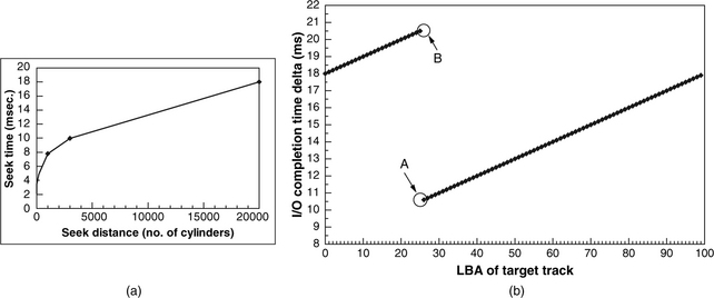
FIGURE 23.10 Seek test example: (a) the seek profile of a hypothetical drive, and (b) the result of the seek test for going from cylinder 0 to cylinder 3000.
While the above measures the seek time going from cylinder 0 to cylinder 3000, the seek time for the reverse direction can also be derived from the same test. Rather than plotting the delta times going from the anchor sector to the target track, plot the delta times going from each sector of the target track to the anchor sector instead. This is illustrated in Figure 23.11. Again, by noting the minimum delta time, the seek time in the reverse direction plus command overheads are measured. In this highly simplified and idealized example, the reverse seek time is identical to the forward seek time. This is not necessarily always true for all disk drives.

Finally, due to mechanical variability, the test pattern should be repeated multiple times to get an average. Also, the test should be repeated using different tracks in the starting and ending cylinders.