
Using a web frontend and built-in graphing is nice and easy, but sometimes, you might want to perform some nifty graphing in an external spreadsheet application or maybe feed data into another system. Sometimes, you might want to make some configuration change that is not possible or is cumbersome to perform using the web interface. While that's not the first thing most Zabbix users would need, it is handy to know when the need arises. Thus, in this chapter, we will find out how to:
- Get raw monitored metric data from the web frontend or database
- Perform some simple, direct database modifications
- Use XML export and import to implement more complex configuration
- Get started with the Zabbix API
Raw data is data as it's stored in the Zabbix database, with minor, if any, conversion performed. Retrieving such data is mostly useful for analysis in other applications.
In some situations, it might be a simple need to quickly graph some data together with another data that is not monitored by Zabbix (yet you plan to add it soon, of course), in which case a quick hack job of spreadsheet magic might be the solution. The easiest way to get data to be used outside of the frontend is actually the frontend itself.
Let's find out how we can easily get historical data for some item. Go to Monitoring | Latest data and select A test host from the Hosts filter field, and then click on Filter. Click on Graph next to CPU load. That gives us the standard Zabbix graph. That wasn't what we wanted, now, was it? But this interface allows us to access raw data easily using the dropdown in the top-right corner—choose Values in there.
If the item has stopped collecting data some time ago and you just want to quickly look at the latest values, choose 500 latest values instead. It will get you the data with fewer clicks.
One thing worth paying attention to is the time period controls at the top, which are the same as the ones available for graphs, screens, and elsewhere. Using the scrollbar, zoom, move, and calendar controls, we can display data for any arbitrary period. For this item, the default period of 1 hour is fine. For some items that are polled less frequently, we will often want to use a much longer period:
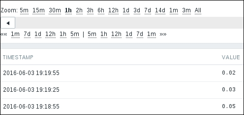
While we could copy data out of this table with a browser that supports HTML copying, then paste it into some receiving software that can parse HTML, that is not always feasible. A quick and easy solution is in the upper-right corner—just click on the As plain text button.
This gives us the very same dataset, just without all the HTML-ish surroundings, such as the Zabbix frontend parts and the table. We can easily save this representation as a file or copy data from it and reuse it in a spreadsheet software or any other application. An additional benefit this data provides—all entries have the corresponding Unix timestamps listed as well.
Grabbing data from the frontend is quick and simple, but this method is unsuitable for large volumes of data and hard to automate—parsing the frontend pages can be done, but isn't the most efficient way of obtaining data. Another way to get to the data would be directly querying the database.
Let's find out how historical data is stored. Launch the MySQL command line client (simply called mysql, usually available in the path variable), and connect to the zabbix database as user zabbix:
$ mysql -u zabbix -p zabbix
When prompted, enter the zabbix user's password (which you can remind yourself of by looking at the contents of zabbix_server.conf) and execute the following command in the MySQL client:
mysql> show tables;
This will list all the tables in the zabbix database—exactly 113 in Zabbix 3.0. That's a lot of tables to figure out, but for our current need (getting some historical data out), we will only need a few. First, the most interesting ones—tables that contain gathered data. All historical data is stored in tables whose names start with history. As you can see, there are many of those with different suffixes—why is that? Zabbix stores retrieved data in different tables depending on the data type. The relationship between types in the Zabbix frontend and database is as follows:
history: Numeric (float)history_log: Loghistory_str: Characterhistory_text: Texthistory_uint: Numeric (unsigned)
To grab the data, we first have to find out the data type for that particular item. The easiest way to do that is to open item properties and observe the Type of information field. We can try taking a look at the contents of the history table by retrieving all fields for three records:
mysql> select * from history limit 3;
The output will show us that each record in this table contains four fields (your output will have different values):
+--------+------------+--------+-----------+
| itemid | clock      | value  | ns        |
+--------+------------+--------+-----------+
|  23668 | 1430700808 | 0.0000 | 644043321 |
|  23669 | 1430700809 | 0.0000 | 644477514 |
|  23668 | 1430700838 | 0.0000 | 651484815 |
+--------+------------+--------+-----------+
The next-to-last field, value, is quite straightforward—it contains the gathered value. The clock field contains the timestamp in Unix time—the number of seconds since the so-called Unix epoch, 00:00:00 UTC on January 1, 1970. The ns column contains nanoseconds inside that particular second.
The first field, itemid, is the most mysterious one. How can we determine which ID corresponds to which item? Again, the easiest way is to use the frontend. You should still have the item properties page open in your browser, so take a look at the address bar. Along with other variables, you'll see part of the string that reads like itemid=23668. Great, so we already have the itemid value on hand. Let's try to grab some values for this item from the database:
mysql> select * from history where itemid=23668 limit 3;
Use the itemid value that you obtained from the page URL:
+--------+------------+--------+-----------+
| itemid | clock      | value  | ns        |
+--------+------------+--------+-----------+
|  23668 | 1430700808 | 0.0000 | 644043321 |
|  23668 | 1430700838 | 0.0000 | 651484815 |
|  23668 | 1430700868 | 0.0000 | 657907318 |
+--------+------------+--------+-----------+
The resulting set contains only values from that item, as evidenced by the itemid field in the output.
One usually will want to retrieve values from a specific period. Guessing Unix timestamps isn't entertaining, so we can again use the date command to figure out the opposite—a Unix timestamp from a date in human-readable form:
$ date -d "2016-01-13 13:13:13" "+%s"
1452683593
The -d flag tells the date command to show the specified time instead of the current time, and the %s format sequence instructs it to output in Unix timestamp format. This fancy little command also accepts more freeform input, such as last Sunday or next Monday.
As an exercise, figure out two recent timestamps half an hour apart, then retrieve values for this item from the database. Hint—the SQL query will look similar to this:
mysql> select * from history where itemid=23668 and clock >= 1250158393 and clock < 1250159593;
You should get back some values. To verify the period, convert the returned clock values back to a human-readable format. The obtained information can be now passed to any external applications for analyzing, graphing, or comparing.
With history* tables containing the raw data, we can get a lot of information out of them. But sometimes, we might want to get a bigger picture only, and that's when table trends can help. Let's find out what exactly this table holds. In the MySQL client, execute this:
mysql> select * from trends limit 2;
We are now selecting two records from the trends table:
+--------+------------+-----+-----------+-----------+-----------+
| itemid | clock      | num | value_min | value_avg | value_max |
+--------+------------+-----+-----------+-----------+-----------+
|  23668 | 1422871200 |  63 |    0.0000 |    1.0192 |    1.4300 |
|  23668 | 1422874800 | 120 |    1.0000 |    1.0660 |    1.6300 |
+--------+------------+-----+-----------+-----------+-----------+
Here, we find two familiar friends, itemid and clock, whose purpose and usage we just discussed. The last three values are quite self-explanatory—value_min, value_avg, and value_max contain the minimal, average, and maximal values of the data. But for what period? The trends table contains information on hourly periods. So if we would like to plot the minimal, average, or maximal values per hour for 1 day in some external application, instead of recalculating this information, we can grab data for this precalculated data directly from the database. But there's one field we have missed: num. This field stores the number of values there were in the hour that is covered in this record. It is useful if you have hundreds of records each hour in a day that are all more or less in line but data is missing for 1 hour, except a single extremely high or low value. Instead of giving the same weight to the values for every hour when calculating daily, weekly, monthly, or yearly data, we can more correctly calculate the final value.
If you want to access data from the database to reuse in external applications, beware of the retention periods—data is removed from the history* and trends* tables after the number of days specified in the History storage period and Trend storage period fields for the specific items.
We covered data retrieval on the Zabbix server. But what if we have a remote site, a Zabbix proxy, a powerful proxy machine, and a slow link? In situations like this, we might be tempted to extract proxy data to reuse it. However, the proxy stores data in a different way than the Zabbix server.
Just like in the previous chapter, run the following command:
$ sqlite3 /tmp/zabbix_proxy.db
This opens the specified database. We can look at which tables are present by using the .tables command:
sqlite> .tables
Notice how there still are all the history* tables, although we already know that the proxy does not use them, opting for proxy_history instead. The database schema is the same on the server and proxy, even though the proxy does not use most of those tables at all. Let's look at the fields of the proxy_history table.
The following table illustrates the item fields and their usage:
As can be seen, several fields will be used for log file monitoring, and some other only for Windows event log monitoring.