
22
Flow Dynamics in Continuous-Time with Average Arc Capacities
Badri Prasad Pangeni1⋆ and Tanka Nath Dhamala2
1Tribhuvan University, Prithvi Narayan Campus, Pokhara, Nepal
2Tribhuvan University, Central Department of Mathematics, Kathmandu, Nepal
Abstract
The dynamics of network flows are influenced by transit time along the arcs, unlike the static cases. A continuous-time model depicts the actual scenario of many transshipment problems. Here, we introduce the average arc problem (AAP) in a continuous-time model which widely occurs in our daily life. In AAP, the flow value which is total of the flow at every time step/instant (in discrete/continuous time respectively) of the arc has an upper bound as the flow capacity of that arc. When the time-expanded network is structured, AAP violates the capacity constraint. This failure of extension of the arc problem (AP) to the AAP of the problem leads to formulating a linear programming of it. In AP, at every instant of time, flow can be sent up to the capacity of that arc, as in the traditional dynamic network flows. To get feasible flow, a transformation and reduction algorithm is also presented.
Keywords: Dynamic network flows, continuous-time model, complexity, linear programming
22.1 Introduction
Consider the water supply network of a city, the traffic network of a highway connecting two cities, or the communication network between two places. In these type of network flows, the capacity of the arc in every time step in discrete time (in every instant in continuous-time) can be fulfilled by the corresponding flows. Ford and Fulkerson [6] introduced such flow dynamics by making dynamic networks with a source and destination. The algorithm with polynomial running time was firstly studied by Hoppe and Tardos [10] and solved flow sending problems in dynamic cases having more than one source and/or sink.
In such cases, if the transit time and capacity of an arc are 5 and 3 units (say) respectively, then each time step can contain 3 units of flow, as shown in Figure 22.1. Here, the capacity is not fulfilled in time steps 1 and 4. We refer to this type of flow problem as the arc problem (AP).
In our paper, we have switched to the cases where some restrictions in each time steps flow cannot be fulfilled. Total value of the flow of all time steps of the transit time of an arc is bounded above by the capacity of that arc (see Figure 22.2), where total of the flow value of time steps 1, 3, and 4 is 3, the capacity of that arc. We call this problem the average arc problem (AAP).
The structure of this paper is as follows. Section 22.2 gives background on how flow dynamics work in a discrete as well as continuous-time setting along with the short view on AAP. In Section 22.3, failure of extension of AP to AAP is discussed with the help of a time-expanded network. A mathematical formulation for the AAP and transformation and reduction algorithm are introduced in Section 22.4. Lastly, the paper is wrapped with conclusion in Section 22.5.
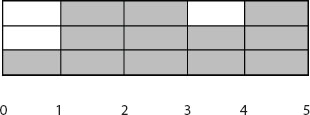
Figure 22.1 Arc with transit time 5 and capacity 3 units.
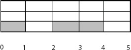
Figure 22.2 Average arc with transit time 5 and capacity 3 units.
22.2 Literature Review
Ford and Fulkerson introduced the notion of network flows in dynamic cases [5, 6]. Gale [7] presented the earliest arrival flow problem. An example in the case of only one source and two sinks having no earliest arrival flow was given by Baumann and Skutella [3]. The quickest flow problem with only one source and single sink related to the maximum flow problem in dynamic status was used by Burkard et al. [4] and also proposed a polynomial as well as strongly polynomial algorithms for the quickest network flow problem.
Dynamic network flow problems with polynomial time complexity were presented by Hoppe and Tardos [9]. Aronson [2] surveyed the network flow problems on discrete dynamic cases, especially on the flow having maximum value. Hamacher and Tjandra [8] focus mainly on building evacuation. Kotnyek [12] also gives a review on dynamic network flows. Kohler et al. [11] introduces the congestion concept on static and dynamic flows.
Network flow problems in continuous-time setting to get maximum flow value were first introduced by Philpott [17] and further extended by Anderson, Nash, and Philpott [1], where they consider the problem without transit times and variable transit and storage capacities. This result with transit time on arc was later extended by Philpott [16].
Skutella [18] presents a survey of dynamic network flows in continuous-time setting with constant transit times and capacities. Nasrabadi and Hashemi [14] investigate a dynamic flow problem having minimum cost with an algorithm where time values are discrete. Pangeni and Dhamala [15] reviewed on dynamic network flows in continuous-time model.
A joint project of the Dahlgren Lab of the U.S. Navy with Cornell University [13] first raised the AAP type problem with the aim to execute an algorithm for solving the AP [10] and to test it on an available data set.
22.3 Failure in Extension of AP to AAP
Consider a directed network N = (V, A) having a set of vertices or nodes V and set of arcs A, such that A ⊂ V × V, i.e., vertices are the crossing-over of arcs.
Let fij: A× [0, T] → R≥0 be a continuous-time dynamic flow in arc (i, j) over the time horizon [0, T], where fij(t) is the rate of flow entering the arc (i, j) in time t. Also, let uij(t), wij(t), and τij(t), respectively, be the capacity of the flow rate, cost of unit flow, and traversal time in arc (i, j) at time t.
Let si: V × [0, T] → R≥0 be a continuous-time dynamic storage at vertex i over [0, T]. Also, let vi(t), xi(t), and mi(t), respectively be the storage capacity, per time unit storage cost per unit flow, and supply/demand rate at vertex or node i, at time t.
Let Fi(t) be the flow rate from supersource ssi to source si(from sink di to supersink sdi) at time t. Also, let Fi be the flow amount supplied from supersupersource sss to supersource ssi (from supersink sdi to supersupersink ssd).
Example. Consider an instance of an AP given in Figure 22.3 and its time-expanded network, respecting the transit times of each arc in Figure 22.4.
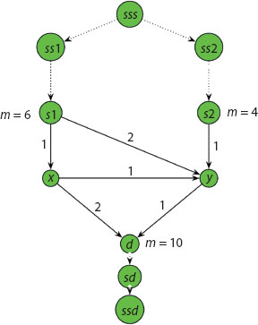
Figure 22.3 Simple instance of dynamic network of an arc problem, arc with transit time, and capacity 1 unit each.
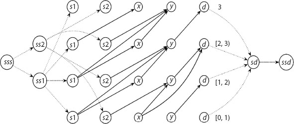
Figure 22.4 Time-expanded network of Figure 22.3 over T = 3.
Consider the flow through the arc (s1, y) in time [0, 1) and [1, 2] and the total flow value is 1 + 1 = 2 units, which violates the capacity of flow in AAP which leads to infeasibility of flow and hence the failure in extension of AP to AAP.
22.4 Formulation
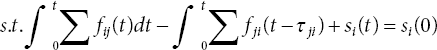
Using the notations introduced above, the minimum time of dynamic flow problem (MTP) suggested by Philpott [16] is:
MTP:
The linear programming formulation for AAP in a discrete-time model formulated by Melkonian [13] is reformulated in a continuous-time model by the authors as follows:
AAP:

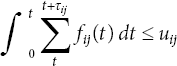
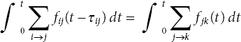
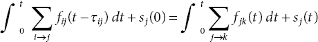


The linear objective function 22.4 aims to minimize the arrival time of the flows at the sink d. Similarly, 22.5, 22.6, 22.7, and 22.8 give capacity constraints of the flows, 22.9 is the flow conservation constraint for intermediate vertex j, 22.10 expresses flow non-conservation constraint, 22.11 and 22.12, respectively, are the conservation constraints for flow in the sources and sinks, 22.13 is the flow conservation constraints for the supersources and supersinks, and lastly 22.14 and 22.15 are the total mass supplied/demanded from supersupersource/supersupersink.
The feasibility of AAP and the above given linear formulation are bi-conditional to each other. To observe the feasibility of flow, the concept of PARTITION is used.
PARTITION Problem
Consider a finite set which has n items with sizes b1,..., bn ∈ Z+, such that ![]() for some J ∈ Z+.
for some J ∈ Z+.
Does some subset I ⊂ {1, ..., n} satisfy the property ![]() ?
?
Theorem 22.1 [13] The necessary and sufficient condition to send two units of dynamic flow from s to d in time T is the existence of a ‘yes’-instance PARTITION problem.
The idea to prove the sufficient part of Theorem 22.1 is the flow of two units is sent along two paths having a disjointed arc in two packets, each having one unit of flow and length n and this can be done in both cases within the prescribed time horizon T. For the necessary part, firstly an arbitrary arc is taken which has more than one unit flow value and total time required to reach the flow to the sink d is calculated which yields more than the time horizon T, which leads to the contradiction. Again, if a supposition is made against the yes instance PARTITION, i.e., ![]() for some Є ≠ 0, then total transit time of the flow on one of the two paths will exceed T.
for some Є ≠ 0, then total transit time of the flow on one of the two paths will exceed T.
If an NP-complete problem fails to be NP-complete after satisfying similarity assumption, then it is called weakly NP-complete. Using the concept of PARTITION and the above theorem, Melkonian [13] showed AAP is NP-complete in the weak sense. To reduce AAP to AP, only the capacities of the arcs are modified, dividing by the corresponding transit times of the arcs where capacity constraints are violated. The following algorithm performs well for the feasibility of flow with the time optimization given by the AAP formulation and its execution steps ahead on the basis of the length of arc having the least transit time.

22.5 Conclusion
When AP is transformed into the time-expanded network, it violates capacity constraints in AAP. This infeasibility of flow leads to the linear formulation of AAP. Using the well-known NP-complete PARTITION problem, AAP is reduced to AP by some modification on arc capacities, i.e, averaging the capacities by the corresponding transit times. The feasibility of reduced AP can be obtained by the algorithm introduced by Hoppe and Tardos [10], implying the feasibility of the original AAP. Practically, the hybrid network would be functioning simultaneously. After observing the feasibility of the flow, the optimality can be obtained by the suitable optimality seeking method (such as network simplex method, etc.).
Acknowledgment
The first author acknowledges University Grants Commission, Nepal for PhD fellowship.
References
- 1. E. J. Anderson, P. Nash and A. B. Philpott (1982). A class of continuous network flow problems. Mathematics of Operation Research, 7: 501-514.
- 2. J. E. Aronson (1989). A survey of dynamic network flows. Annals of Operations Research, 20: 1-66.
- 3. N. Baumann and M. Skutella (2006). Solving evacuation problems efficiently–earliest arrival flows with multiple sources. In: 47th annual IEEE symposium on foundations of computer science (FOCS’06), 399–410.
- 4. R. Burkard, K. Dlaska and B. Klinz (1993). The quickest flow problem. ZOR Meth Models Oper Res, 37: 31–58.
- 5. L. R. Ford and D. R. Fulkerson (1958). Constructing maximal dynamic flows from static flows. Operations Research Letters, 6: 419-433.
- 6. L. R. Ford and D. R. Fulkerson (1962). Flows in networks. Princeton University Press, New Jersey.
- 7. D. Gale(1959). Transient flows in networks. Michigan Math J, 6(1): 59–63.
- 8. H. Hamacher and S. Tjandra (2001). Mathematical modeling of evacuation problems: a state of art. Berichte des Frauenhofer ITWM, Nr. 24. http://www.itwm.fraunhofer.de/fileadmin/ITWMMedia/Zentral/Pdf/BerichteITWM/2001/bericht24.pdf. Accessed 18 Oct 2006.
- 9. B. Hoppe and E. Tardos (1994). Polynomial time algorithms for some evacuation problems. In: Proceedings of the fifth annual ACM-SIAM symposium on discrete algorithms, Society for Industrial and Applied Mathematics Philadelphia, PA, 433–441.
- 10. B. Hoppe and É. Tardos (2000). The quickest transshipment problem. Mathematics of Operations Research 25: 36–62.
- 11. E. Kohler, R. H. Mohring, and M. Skutella (2009). Traffic networks and flows over time. In: Lerner J, Wagner D, Zweig K (eds) Algorithmics of large and complex networks. Lecture notes in computer science, vol 5515. Springer, Berlin, 166–196.
- 12. B. Kotnyek (2003). An annotated overview of dynamic network flows. INRIA, Sophia Antipolis, France.
- 13. V. Melkonian (2007). Flows in dynamic networks with aggregate arc capacities. Information Processing Letters 101: 30–35.
- 14. E. Nasrabadi and S. M. Hashemi (2010). Minimum cost time-varying network flow problems. Optim Meth Software, 25(3): 429–447.
- 15. B. P. Pangeni and T. N. Dhamala (2021). A brief survey on dynamic network flows in continuous-time model. Journal of Mathematical Sciences and Computational Mathematics 2(4): 467-477.
- 16. A. B. Philpott (1990). Continuous-time flows in networks. Mathematics of Operation Research, 15: 640-661.
- 17. A. B. Philpott (1982). Algorithms for continuous network flow problems. Ph.D. thesis, University of Cambridge UK.
- 18. M. Skutella (2009). An introduction to network flows over time. In W. Cook, L. Lovasz and J. Vygen (eds.): Research Trends in Combinatorial Optimization, Springer, Berlin, 451-482.
Note
- ⋆ Corresponding author: [email protected]