
Chapter Six
Small-Scale Dish-Mounted Solar Thermal Brayton Cycle
Abstract
The small-scale dish-mounted solar thermal Brayton cycle in the 1- to 20-kW range has several advantages such as mobility, bulk manufacturing, cogeneration, and hybridization. Another advantage is that an off-the-shelf turbocharger from the motor industry can be applied as the microturbine in the cycle. The main disadvantages are low turbine and compressor efficiencies as well as heat and pressure losses. The chapter shows that the method of total entropy generation minimization can be used to maximize the net power output of the cycle by optimizing an open-cavity tubular solar receiver and counterflow plate-type recuperator. Results show that, with the use of an off-the-shelf turbocharger and low-cost optics, the cycle could generate solar-to-mechanical efficiencies of up to 12% with much room for improvement. Remaining challenges and future possibilities are discussed. It is recommended that the cycle should be further developed and investigated as a clean energy technology.
Keywords
Brayton; Dish; Receiver; Recuperator; Solar; Turbocharger
6.1. Introduction
Solar power generation holds endless opportunities for countries in solar-rich areas; however, more efficient and cost-effective small-scale solar-to-electricity technologies are required. The small-scale dish-mounted solar thermal Brayton cycle (STBC), shown in Fig. 6.1, using a recuperator and an off-the-shelf turbocharger has the potential for high energy conversion efficiency. The closed Brayton cycle was developed in the 1930s for power applications and was adapted to the design and development of STBCs for space power in the 1960s, with the success of lightweight and high-performance gas turbines for aircraft [1]. The STBC in the 1- to 20-kW range can be applied to generate power for small communities.

The parabolic dish reflects and concentrates the sun's rays onto the receiver aperture so that solar heat can be absorbed by the inner walls of the receiver. With reference to Fig. 6.1, the compressor (1–2) increases the air pressure before it is heated in the recuperator (3–4) and solar receiver (5–6). In the recuperator, hot turbine exhaust air (9–10) is used to preheat the compressed air. The compressed and heated air expands in the turbine (7–8), which produces rotational shaft power for the compressor and the electric load. The compressor, turbine, and generator are mounted on a single shaft and all spin at the same rate [2,3]. It is simple, robust, and easy to maintain. A recuperated STBC allows for lower compressor pressure ratios [4], higher efficiency [1], and a less complex solar receiver, which operates at lower pressure.
The open Brayton cycle uses air as working fluid, which makes this cycle very attractive for use in water-scarce countries. The hot exhaust air coming from the recuperator can be used for cogeneration, such as water heating. The use of cogeneration makes the cycle more efficient and highly competitive. Intercooling and reheating can also be applied to increase efficiency. The use of local small-scale power generation means that transmission lines do not have to cross vast stretches of land to bring electricity to isolated areas.
The STBC can be supplemented with natural gas as a hybrid system [5] for continuous operation when the sun is not shining. Storage systems such as packed rock bed thermal storage [6] can also be coupled to the cycle. Cameron et al. [7] showed how lithium fluoride could be used in the solar receiver of an 11-kW earth-orbiting STBC with recuperator to store heat for as much as 38 min during full power operation. The small-scale dish-mounted STBC also has an advantage in terms of bulk manufacturability and cost. Microturbines can be adapted as turbochargers from the vehicle market off the shelf [8], which allows for lower costs due to high production quantities [9].
According to Pietsch and Brandes [1], experimental testing of the STBC has proved high reliability and efficiencies above 30% with turbine inlet temperatures of between 1033K and 1144K. Dickey [10] also presented experimental test results of an STBC (20–100 kW), an initiative from HelioFocus Ltd. and Capstone Microturbine at the Weizmann Institute. A proprietary pressurized volumetric solar receiver was used in the experiment. A system efficiency of 11.76% was achieved with a solar receiver exit temperature of 871°C. The system generated 24.04 kW of electricity with the microturbine spinning at 96,000 rpm. Heller et al. [11] tested an open STBC without a recuperator and found that a volumetric pressurized receiver can produce air of 1000°C to drive a gas turbine. According to [11], the cost and performance of this cycle looks promising for future solar power generation. According to Chen et al. [12], the Brayton cycle is definitely worth studying when comparing its efficiency with those of other power cycles. Mills [9] predicted that small-scale Brayton microturbines might become more popular than Stirling engines due to high Stirling engine costs.
As shown earlier, the STBC has much potential and its efficiency can be improved using various methods. Another method to improve the efficiency of the cycle is through design optimization. When designing the STBC, there is a compromise between allowing effective heat transfer and keeping pressure losses in the components small. Heat losses and pressure losses in the components of the cycle decrease the net power output of the cycle. Limiting factors to the performance of the STBC include maximum receiver surface temperature and recuperator weight. The Brayton cycle and the optimization thereof have been studied by many authors; however, not many have studied the STBC with recuperator. Zhang et al. [13], for example, studied the performance of a closed STBC without a recuperator. Solar receivers and recuperators have been designed and optimized individually for the Brayton cycle and the STBC [14–16]; however, various studies such as [17] have emphasized the importance of the optimization of the global performance of a system, instead of optimizing components individually. To obtain the maximum net power output of the cycle, a combined effort of heat transfer, fluid mechanics, and thermodynamic thought is required. The method of entropy generation minimization combines these thoughts [18]. Jubeh [19] has done an exergy analysis of specifically the open STBC with recuperator.
Optimization of the geometry variables of cycle components using the method of total entropy generation minimization is considered to be a holistic optimization approach and has been applied to the STBC in recent work for maximum net power output [20–23]. In this chapter, the method is applied to a recuperated STBC with low-cost dish optics and low-cost tracking. Furthermore, three different off-the-shelf turbochargers from Garrett [8] are investigated for use in the STBC.
6.2. Solar Collector and Receiver
Dish manufacturing and installation errors influence the position and shape of the focal point of the dish. Due to these errors and due to the sun's rays not being truly parallel, the reflected rays from the dish form an image of finite size centered on its focal point. The accuracy of the solar tracking system and the quality of the optics are important factors in the total cost of the small-scale dish-mounted STBC. Two-axis solar tracking is required to ensure that the sun's rays stay focused on the receiver aperture throughout a typical day. Typical solar tracking errors are between 0.1° and 2° [24]. The tracking accuracy is much dependent on sensor alignment, base-level alignment, momentum of the moving dish, and also drive nonuniformity and receiver alignment [4]. Error due to wind loading is also a measurable quantity [25]. For the dish, good reflectance and specular reflection of the entire terrestrial solar spectrum are important. Typical specularity errors range between 0 and 3.84 mrad, whereas typical slope errors are 1.75, 3, and 5 mrad [26]. The specular reflectance of any material is a function of time, regardless of the reflector [4].
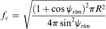
According to Ref. [4], the focal length of a parabolic dish is defined by Eq. (6.1). The rim angle of a parabolic dish determines where its focal point is. A rim angle of 45° is paramount for concentrators with focal plane receivers [4].
 (6.1)
(6.1)
Solar receivers can be divided into tubular, volumetric, and particle receivers. A number of high-temperature and high-efficiency receivers are available from the literature, mostly for use in large-scale (10–200 MW) applications [27,28]. Typical receiver efficiencies and experimental data that have been obtained with pressurized volumetric receivers and tubular receivers are summarized in Ref. [24]. These receivers are mostly not optimized to perform well in a dish-mounted STBC with recuperator. A solar receiver might be designed for high efficiency, but if it is not optimized to achieve a common goal together with other components, it might not perform well in a recuperated Brayton cycle.
Most Brayton cycles are not self-sustaining at operating temperatures below 480°C [4]. For the STBC, the maximum receiver surface temperature and turbine inlet temperature are very important. The higher these temperatures, the better the Brayton cycle will perform, but more heat will be lost to the environment [21]. The maximum turbine inlet temperature of commercial off-the-shelf turbochargers is more or less 950°C [8,29], whereas for ceramic microturbines a temperature of 1170°C is envisaged [30]. The higher the turbine inlet temperature, the less material choices are available for the receiver.
6.3. The Tubular Open-Cavity Receiver
For simplicity and ease of optimization, a tubular open-cavity receiver [24] is considered in this work. Overall collector efficiencies of between 60% and 70% [31] are attainable with state-of-the-art open-cavity receivers operated in the temperature range of 500°C–900°C with an optimum area ratio of 0.0004 ≤ A′ ≤ 0.0009. The receiver efficiency is defined as shown in Eq. (6.2). Eq. (6.3) shows the overall efficiency of the STBC.
![]() (6.2)
(6.2)
![]() (6.3)
(6.3)
The open-cavity tubular solar receiver (see Fig. 6.2) consists of a coiled stainless steel tube through which pressurized air travels. The depth of the receiver is equal to 2a. The receiver is covered with ceramic fiber insulation. Reflected solar beam irradiance gets absorbed at the inner walls of the cavity. The receiver has been tested at low temperatures in a low-cost solar dish with the use of weld-on thermocouples [32].

Figure 6.2 An open cavity solar receiver in section view (left) and from the side (right) [32].
The heat loss from the receiver consists of convection, radiation, and conduction and can be modeled with the Koenig and Marvin heat loss model [33] presented by Harris and Lenz [31]. The heat loss per tube section is determined with Eq. (6.4). The larger the cavity aperture, the more heat can be lost, but more heat can also be intercepted.
![]() (6.4)
(6.4)
6.3.1. Conduction Heat Loss
The conduction heat loss rate through the insulation is calculated per tube section with Eq. (6.5) and Eq. (6.6) [24]. Eq. (6.6) was obtained by assuming an average wind speed of 2.5 m/s, an insulation thickness of tins = 0.1 m and an average insulation conductivity of 0.061 W/mK at 550°C [24,31]. The convection heat transfer coefficient on the outside of the insulation was determined by assuming a combination of natural convection and forced convection due to wind [24].
![]() (6.5)
(6.5)
![]() (6.6)
(6.6)
6.3.2. Radiation Heat Loss
The radiation heat loss rate from the receiver aperture is calculated per tube section in Eq. (6.7) [24]. The radiation heat loss and gain at each part of the inner wall is determined with the use of Eq. (6.8), where the view factors for the receiver are available from Ref. [24].
![]() (6.7)
(6.7)
 (6.8)
(6.8)
6.3.3. Convection Heat Loss
The convection heat loss rate from the open cavity receiver is determined per tube section according to Eq. (6.9) [31], where the natural convection heat transfer coefficient is determined according to Ref. [24]. The natural convection heat transfer coefficient according to Ref. [24] is hinner = 2.75 W/m2K and a wind effect constant of w = 2 can be assumed.
![]() (6.9)
(6.9)
6.3.4. Optimization and Efficiency
There are many different variables at play to model the efficiency of the receiver. These variables include concentrator shape, concentrator diameter, concentrator rim angle, concentrator reflectivity, concentrator optical error, tracking error, receiver aperture area, receiver material, receiver tube diameter, inlet temperature, and mass flow rate through the receiver.
The factors contributing to the temperature profile and net heat transfer rate on the receiver tube can be divided into two components: geometry dependent and temperature dependent. The geometry-dependent factors include the concentrator dish with its optics: tracking error, specularity error, slope error, reflectance, spillage, and shadowing. The effects of these factors can be found with the use of ray-tracing software. Computer software and algorithms as described by Ho [34] and Bode and Gauché [35] are available to compute the solar heat flux on a receiver as reflected from a reflector.
Regarding the temperature-dependent factors, a method to determine the receiver tube surface temperature and net heat transfer rate along the length of the receiver tube is described in Ref. [24], as shown in Eqs. (6.10) and (6.11). Eq. (6.10) is derived from Eq. (6.4).
 (6.10)
 (6.11)
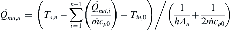
The heat loss terms in Eq. (6.10) can be linearized as shown in Eq. (6.12). By using Gaussian elimination, Eq. (6.11) and Eq. (6.12) can be solved simultaneously to determine the temperature profile (Ts,n) of the receiver tube and the net absorbed heat rate ( ) at each tube section [24].
 (6.12)
In Eq. (6.12),  can be determined with the use of a ray-tracing software such as SolTrace (see Fig. 6.3). SolTrace is a software tool developed at the National Renewable Energy Laboratory to model concentrating solar power optical systems and analyze their performance. The optical error of the dish is determined from the slope error and specularity error as shown in Eq. (6.13).
![]() (6.13)
(6.13)
6.4. Recuperator
The addition of a recuperator in the cycle allows for a higher efficiency, a lower operating pressure, and a less complex receiver. The recuperator is used to preheat air going to the solar receiver by extracting heat from the turbine exhaust air (see Fig. 6.1). Heat exchangers are required to be efficient, safe, economical, simple, and convenient [36]. It is often beneficial for the cycle to have a large recuperator; however, the recuperator should be practical. Heat transfer and pressure losses as well as the optimization of cost, weight, and size should be considered when designing a heat exchanger [37]. The recuperator should have high effectiveness, compactness, 40,000-h operation life without maintenance, and low pressure loss (<5%) [29]. These criteria translate into a thin foil primary surface recuperator where flow passages are formed with stamping, folding, and welding side edges by an automated operation [29,38,39]. In solar applications, a compact counterflow recuperator [18,40,41] with multiple flow channels is often designed as integral to the microturbine. With the use of multiple flow channels, heat exchanger irreversibilities can be decreased by slowing down the fluid that is traveling through the heat exchanger [18].

A counterflow plate-type recuperator is considered as shown in Fig. 6.4 [22]. The channels with length Lreg and aspect ratio a/b are shown. The recuperator effectiveness is modeled using an updated ε-NTU (effectiveness – number of transfer units) method [42]. This method takes the heat loss to the environment into consideration when calculating the recuperator efficiency, since the recuperator operates at a very high average temperature. According to Ref. [42], the hot side and cold side efficiencies can be calculated with Eq. (6.14) and Eq. (6.15) and the equations below.
 (6.14)
 (6.15)

 (6.16)
![]() (6.17)
(6.17)
![]() (6.18)
(6.18)
![]() (6.19)
(6.19)
 (6.20)
 (6.21)
The heat loss rate from the hot side and cold side of the recuperator is calculated with Eq. (6.22) and Eq. (6.23) and the following equations.
![]() (6.22)
(6.22)
![]() (6.23)
(6.23)
![]() (6.24)
(6.24)
![]() (6.25)
(6.25)
![]() (6.26)
(6.26)
![]() (6.27)
(6.27)
6.5. Turbocharger as Microturbine
The compressor isentropic efficiency, compressor corrected mass flow rate, compressor pressure ratio, and rotational speed are intrinsically coupled to each other and are available from the compressor map [8,43]. Compressor and turbine maps from standard off-the-shelf turbochargers from Garrett [8] are considered. The compressor isentropic efficiency and shaft speed is obtained with interpolation. The compressor should operate within its compressor map range, otherwise flow surge or choking can occur. According to Ref. [23], the turbine efficiency is determined by calculating the blade speed ratio [44–46] as shown in Eq. (6.28) and Eq. (6.29). The blade speed ratio is a function of the inlet enthalpy, pressure ratio, turbine wheel diameter, and rotational speed [23,45]. According to Guzzella and Onder [47], in automotive applications, typical values for the maximum turbine efficiency are  . Note that the system mass flow rate is equal to the actual turbine mass flow rate and is calculated with Eq. (6.30) where P7 is in pounds per square inch and T7 is in degrees Fahrenheit, respectively [8].
 (6.28)
 (6.29)
 (6.30)
6.6. Optimization and Methodology
The method of entropy generation minimization is used to maximize the net power output of the STBC at steady state by optimizing the geometry variables of the receiver and recuperator [23]. When considering geometric optimization of components, in a system using a turbomachine, the compressor or turbine pressure ratio can be chosen as a parameter [48–50]. In this work, the turbine operating point (turbine corrected mass flow rate and turbine pressure ratio) is chosen. Note that the turbine corrected mass flow rate is a function of the turbine pressure ratio according to the turbine map.
![]() (6.31)
(6.31)
 (6.32)
The finite heat transfer and pressure drop in the compressor, turbine, recuperator, receiver, and other tubes are identified as entropy generation mechanisms. When doing an exergy analysis of the system at steady state and assuming V1 = V11 and Z1 = Z11 (see Fig. 6.1), the objective function is assembled as shown in Eq. (6.31). The function to be maximized (the objective function), is  (the net power output). Eq. (6.32) shows the total entropy generation rate in terms of the temperatures and pressures at different locations in the cycle (with reference to Fig. 6.1). The entropy generation rate of each component is added as shown in Eq. (6.32). T∗ is the apparent sun's temperature as an exergy source as described in Ref. [23]. Note that
  . For validation, the net power output can also be calculated with the first law of thermodynamics using a control volume around the microturbine and also around the system.
As optimization, different combinations of three turbochargers by Garrett [8], three different receiver tube diameters, and 625 differently sized recuperators are used as parameters and variables to determine the net power output of the system. MATLAB [51] is used to determine the variables that will give the best results. The recuperator variables are the width of the recuperator channel, a, the height of a recuperator channel, b, the length of the recuperator, L, and the number of flow channels in one direction, n. The maximum receiver surface temperature is constrained to 1200K. The recuperator total plate mass is restricted to 300, 400, or 500 kg. The temperatures and pressures at every point of the STBC are found with iteration and by modeling every component [23] and using isentropic efficiencies of the compressor and turbine as well as recuperator and receiver efficiencies.
6.6.1. Assumptions
It is assumed that the receiver and recuperator are made from stainless steel. The pressure drop through the receiver tube and other tubes in the cycle is calculated with the friction factor using the Colebrook equation [52] for rough stainless steel. The pressure drop through the recuperator is calculated similarly or by using the friction factor for fully developed laminar flow, depending on the Reynolds number. It is assumed that T8 = T9 and P8 = P9 since the recuperator and microturbine are close to each other. It is further assumed that T2 = T3 and P2 = P3 since the recuperator and microturbine are close to each other. Also note that T1 = 300K and P1 = P10 = P11 = 86 kPa. It is assumed that the thickness of the material between the hot and cold stream, t, in the recuperator, is 1 mm.
6.7. Results
With the use of SolTrace, Fig. 6.5 is obtained as an initial result, showing the effect of the aperture size and the optical error on the receiver efficiency [24]. An average receiver surface temperature of 1150 K was assumed to estimate the heat loss. A pillbox sunshape parameter of 4.65 mrad was assumed in the SolTrace analysis and a parabolic dish rim angle of 45°. The reflectance of the receiver tube was assumed to be 15% (oxidized stainless steel) and the emissivity of the receiver material as 0.7. It was mentioned previously that the dish optics and tracking errors are important factors regarding the total cost of the system. A solar tracking error of 1° was used in the analysis. A tracking error of 1° indicates rather poor tracking and thus a low-cost tracking system. Note that an optimum area ratio exists for each optical error in Fig. 6.5. If an optical error of 10 mrad is assumed, the optimum area ratio is A′ ≈ 0.0035 [24].

Figure 6.5 Overall receiver efficiency for a tracking error of 1° with receiver surface emissivity of 0.7 [24].
In the following results, a solar dish with diameter of 4.8 m was considered and a solar direct normal irradiance (DNI) of 1000 W/m2 was assumed. For a fixed area ratio of A′ = 0.0035, the available solar power at the aperture of a receiver with a = 0.25 m (aperture area of 0.25 m × 0.25 m) is shown in Fig. 6.6 for different tracking errors and optical errors. Fig. 6.6 shows that the available solar power decreases as the optical error and tracking error increase. However, at a tracking error of 3°, the available solar power increases as the optical error increases, since the focal image increases as the optical error increases. Note that the available solar power stays almost constant when the tracking error is between 0° and 1° and the optical error below 10 mrad.
Fig. 6.7 shows the average net heat transfer rate at the cavity receiver inner wall. The net heat transfer rate is the available solar power minus the heat loss rate from the cavity receiver to the environment. Note that a dish reflectivity of 85% was assumed. Fig. 6.7 also shows that an optical error of 10 mrad or less with a tracking error of 1° or less is required to have an acceptable net heat transfer rate. A tracking error of 2° would thus not be acceptable for the collector.
Eq. (6.31) was used as an objective function in MATLAB to determine the maximum net power output of the cycle by optimizing the receiver tube diameter and counterflow plate-type recuperator geometries. A 4.8-m-diameter parabolic dish, rim angle of 45°, 1° tracking error, 10 mrad optical error, a = 0.25, solar receiver emissivity of 0.7, a solar DNI of 1000 W/m2, and a dish reflectivity of 85% was used to generate the results. It was also assumed that all tubing in the cycle has 10 mm insulation thickness and conduction heat transfer coefficient of 0.18 W/mK. For the open-cavity tubular receiver, efficiencies of between 43% and 70% were obtained with mass flow rates of between 0.06 and 0.08 kg/s, tube diameters of between 0.05 and 0.0889 m, and air inlet temperatures of between 900K and 1070K [24]. In Figs. 6.8–6.10 the maximum net power output of the STBC at steady state was found as a function of turbine pressure ratio. It is shown that the maximum net power output of the system can be found when a large receiver tube diameter is used, for all three of the microturbines. Note that each data point represents a maximum, which is achieved using a unique recuperator as shown in Table 6.1 for the GT2860RS turbocharger with a receiver tube diameter of 0.0833 m (compare with Fig. 6.9). From Table 6.1, a recuperator with a = 0.225 m, b = 2.25 mm, L = 1.5 m, and n = 45 was the best-performing recuperator since it gave the highest maximum net power output of 1.77 kW (Table 6.1). Note that in these results the recuperator mass was restricted to 500 kg and the receiver surface temperature restricted to 1200K.


Figure 6.7 The average net heat transfer rate at the open-cavity receiver inner walls with a = 0.25 m.
The GT1241 provides the highest maximum power output of 2.11 kW and a conversion efficiency of 12% (Fig. 6.10). This efficiency compares well with photovoltaic panels. It should be noted that this efficiency can be improved in many ways. Note that in this chapter, low-cost tracking and solar optics were considered, which decrease the efficiency of the receiver. In this work, only standard off-the-shelf turbochargers were considered, which are not necessarily optimized to perform as a power-generating unit but rather for performance in a vehicle. However, the low cost of these units justifies the research into its application in this field. Further investigation into the correct matching of turbocharger compressors and turbines to improve efficiency should be done. The overall efficiency of the cycle can also be improved with the use of cogeneration. It should also be noted that higher efficiencies have already been obtained with state-of-the-art systems, as mentioned in Section 6.1.


For larger receiver tube diameters, a higher maximum net power output can be achieved at high turbine pressure ratios. Note that in Ref. [24], it was found that the highest second law efficiencies for the receiver were achieved when the tube diameter and inlet temperature were large and the mass flow rate small. This combination of variables would also create a very high surface temperature. When the surface temperature is then restricted to 1200K, a larger mass flow rate and lower inlet temperature can still provide high second law efficiencies, when a large tube diameter is chosen.
Table 6.1
Optimum Recuperator Geometries, Maximum Net Power Output, Maximum Receiver Surface Temperature, and Recuperator Mass for GT2860RS With Receiver Tube Diameter D = 0.0833 m
| rt | a (m) | b (mm) | L (m) | n | Ts,max (K) | Mass (kg) | |
| 1.25 | 0.15 | 4.5 | 1.5 | 22 | 470 | 1186 | 167 |
| 1.313 | 0.37 | 4.5 | 1.5 | 15 | 843 | 1197 | 273 |
| 1.375 | 0.37 | 3.7 | 1.5 | 22 | 1319 | 1195 | 409 |
| 1.438 | 0.45 | 3.0 | 1.5 | 22 | 1524 | 1180 | 489 |
| 1.5 | 0.22 | 2.2 | 1.5 | 45 | 1767 | 1127 | 491 |
| 1.563 | 0.45 | 2.2 | 1.5 | 22 | 1736 | 1053 | 488 |
| 1.625 | 0.22 | 2.2 | 1.5 | 45 | 1655 | 1000 | 491 |
| 1.688 | 0.22 | 2.2 | 1.5 | 45 | 979 | 940 | 491 |
| 1.75 | 0.22 | 2.2 | 1.5 | 45 | 597 | 885 | 491 |
| 1.813 | 0.22 | 2.2 | 1.5 | 45 | 90 | 830 | 491 |

The larger the mass of the recuperator, the higher the net power output of the system as shown in Fig. 6.11. When the recuperator mass is constrained to 400 kg, a recuperator with a = 150 mm, b = 2.25 mm, L = 1.5 m, and n = 45 was found to be the recuperator with the most common optimum dimensions. When the recuperator mass is constrained to 300 kg, a recuperator with a = 150 mm, b = 2.25 mm, L = 1.5 m, and n = 37.5 is best.
From Fig. 6.12 it is shown that it is optimum for the maximum receiver tube surface temperature to decrease with increasing turbine pressure ratio and with decreasing receiver tube diameter. At high turbine pressure ratios, the large receiver tube diameter has a higher surface temperature and it allows for higher net power output of the small-scale STBC.


6.8. Remaining Challenges and Future Possibilities
The smaller a microturbine, the higher its operating speed. Off-the-shelf commercial turbochargers operate at speeds of 50,000–180,000 rpm [8]. A remaining challenge for the STBC using an off-the-shelf turbocharger is to connect the turbocharger's shaft to a high-speed generator that generates electric power of high and variable frequency before it is rectified to direct current [2]. Shiraishi and Ono [3] showed that a flexible coupling can be used to connect the turbocharger and generator. A two-shaft configuration can also be considered. According to Weston [53], the two-shaft arrangement allows for acceptable performance over a wider range of operating conditions. In the case where two-shaft technology is considered, the addition of reheating and intercooling, which is usually present on two-shaft configurations and which makes the cycle much more efficient, becomes more attractive. The possible commercial availability of high-speed gearboxes in future will invalidate the need for a high-speed generator and will allow for a low-speed generator to be coupled directly to the turbine shaft.
Future possibilities of the STBC include hybridization and thermal storage for continuous power generation, as was also mentioned in Section 6.1. Hot exhaust air leaving the STBC can be used to heat water or to run an absorption chiller. If the exhaust gas is not utilized, it is very important that the exhaust air is exposed of correctly and that it is not sucked in again at the compressor. Furthermore, commercial turbine operating temperatures might be increased in future with the use of ceramic materials, which will allow for higher STBC efficiencies.
6.9. Conclusion and Recommendations
The small-scale dish-mounted STBC using a turbocharger as microturbine is a technology with a lot of potential to generate electricity from solar power. The chapter discussed the potential of the technology as well as the remaining challenges. One of the important advantages of the cycle is that it can be supplemented with natural gas as a hybrid system for continuous operation when solar radiation levels are low or during the night.
The cycle is faced with low compressor and turbine efficiencies, heat losses, and pressure losses, which decrease the net power output of the system. In this chapter, a recent development in the minimization of these losses was presented. The power output of the small-scale dish-mounted STBC with recuperator, off-the-shelf turbocharger, and low-cost optics was modeled and maximized using the method of total entropy generation minimization. A receiver and recuperator were optimized to perform in the cycle. Results showed that higher maximum net power output can be achieved at high turbine pressure ratios, when a large receiver tube diameter is used. It was found that a recuperator with a = 225 mm, b = 2.25 mm, L = 1.5 m, and n = 45 gives the best results for the setup with the recuperator mass constraint and receiver maximum surface temperature constraint. The larger the mass of the recuperator, the higher the power output of the system.
Results showed that solar-to-mechanical efficiencies of up to 12% could be achieved when using a standard off-the-shelf turbocharger and low-cost optics. The efficiency is low compared with other solar technologies; however, there are many ways in which the efficiency can be improved. Note that the current work only considered commercial turbochargers with an already-combined compressor and turbine. This combination is chosen for performance in a vehicle rather than for power generation. Further compressor and turbine matching should be performed to identify better combinations of these units for significant efficiency improvement. It should also be noted that a very simple solar receiver was used for the modeling. With the use of high absorptivity and low emissivity coatings, the efficiency of the receiver can be increased. It is recommended that high-temperature, low-emissivity receiver coatings and materials should be investigated further experimentally to improve efficiency. The efficiency can be further improved by having more precise tracking and dish optics and higher dish reflectivity. Note that, in this chapter, a receiver aperture area of 0.25 m × 0.25 m and a dish with poor tracking (1° error) and poor dish optics (10 mrad error) were assumed. According to Ref. [24], the receiver efficiency can be increased up to 71% when both the optical error and tracking error are changed to 5 mrad and 0°, respectively, and the aperture area to 0.1 m × 0.1 m. By adding water heating using the hot exhaust air, the overall efficiency will be increased even further.
Furthermore, it is recommended that a cost-versus-efficiency study should be done regarding the small-scale dish-mounted STBC. With further research, the small-scale open STBC could become a competitive off-the-grid small-scale solar energy solution for small communities. It is recommended that the cycle should be further developed experimentally and investigated as a clean energy technology.
Nomenclature
a Receiver aperture side length or recuperator channel width, m
b Recuperator channel height, m
A Area, m2
A′ Receiver aperture to dish area ratio
BSR Blade speed ratio
c1 Constant used in linear equation
c2 Constant used in linear equation
cp0 Constant pressure specific heat, J/kgK
Cr Capacity ratio
D Diameter, m
fc Focal length, m
F View factor
h Heat transfer coefficient, W/m2K
h Specific enthalpy, J/kg
H Recuperator height, m
k Thermal conductivity, W/mK
k Gas constant
L Length, m
m1 Slope of linear equation
m2 Slope of linear equation
M Mass of recuperator, kg
n Number of recuperator flow channels in one direction
N Number of tube sections
N Speed of microturbine shaft, rpm
NTU Number of transfer units
P Pressure, Pa
r Pressure ratio
R Gas constant, J/kgK
R Dish radius, m
R Thermal resistance, K/W
t Thickness, m
T Temperature, K
T∗ Apparent exergy-source sun temperature, K
U Overall heat transfer coefficient, W/m2K
w Wind factor
V Velocity, m/s
X Dimensionless position
Z Height, m
Greek Letters
ɛ Emissivity of receiver
ɛ Recuperator effectiveness
η Efficiency
Θ Dimensionless temperature difference
σ Stefan–Boltzmann constant, W/m2K
χ Dimensionless external heat load
ψrim Rim angle
ω Error, mrad
Subscripts
0 Initial inlet to receiver
1–11 Refer to Fig. 6.1
ap Aperture
BC Brayton cycle
bottom At the bottom
c Compressor
c Based on the cold side
CF Corrected flow
col Collector
cond Due to conduction
conv Due to convection
e Exit
h Based on the hot side
i Inlet
in At the inlet
ins Insulation
int Internal
inner On the inside
l Loss
max Maximum
n Tube section number
net Net output
opt Optimum
optical Optical
out On the outside of the insulation
rad Due to radiation
rec Receiver
refl Due to dish reflectivity
REC For the receiver including optical efficiency
reg Recuperator
s Surface
side At the side
slope Slope
solar From solar as determined with SolTrace
specularity Specularity
STBC Solar thermal Brayton cycle
t Turbine
top At the top
∞ Environment
..................Content has been hidden....................
You can't read the all page of ebook, please click here login for view all page.